Introduction

Large-scale features of the polar regions, such as continental ice sheets, are sensitive to climate change on time-scales ranging from decades to millennia, and react to the effects of other components of the climate system that vary on time-scales ranging from seconds to millions of years. The mechanisms involved in the land–sea-ice processes that affect ice sheets are poorly understood, yet are important to understanding both the decadal-scale human influences on climate and the response of the continental ice sheets to variations in the Earth's orbital parameters on the 10 000–100000 year time-scales. In order to examine these processes in more detail we have developed a coupled energy-balance climate–thermodynamic sea-ice–continental-ice-sheet model (CCSLI model; Reference SteenSteen, 1995). This model couples a model that includes a hydrologic cycle, a detailed surface-energy balance, horizontal energy transports, and a thermodynamic sea-ice model (CCSI model; Reference LedleyLedley 1991; Reference Chu and LedleyChu and Ledley, 1995) with a zonally averaged dynamic land–ice-flow model with bedrock response (Reference Birchfield and GrumbineBirchfield and Grumbine, 1985). The energy and mass-balance calculations in the CCSLI model permit an examination of the mechanisms involved in the interactions between the different components of the climate system, making the CCSLI model an excellent tool with which to investigate long-term ice age variations.

Since a large range of space and time-scales are inherent to this model, and because it will be used to examine climate change over a long period of time, requiring large amounts of computer time, an asynchronous coupling scheme has been developed. The asynchronous coupling is done in two parts, which take advantage of the long time constant of the ice sheets and the fast response time of the atmosphere to changes in the ice-sheet configuration.

Previous work by Reference Pollard, Muszynski, Schneider and ThompsonPollard and others (1990) evaluated similar asynchronous coupling schemes between ice-sheet models and atmospheric forcing. Their work used a prescribed pattern of net accumulation and ablation, defined

by an equilibrium line that was shifted up and down in response to long-term orbital variations, stochastic inter-annual weather variability, and ice-sheet albedo feedback. The goal of their work was to study the implications of ice-sheet-atmospheric couplings in general circulation model (GCM) studies. Indeed, estimates from this work show that the computer costs associated with simulating one glacial interglacial cycle would be reduced from over 100 year's supercomputer (CRAY X-MP/48) CPU time to around 1.7 years of CPU time. We show that the CCSLI model can simulate 150 000 years in about 12 hours.

The computational expense of GCMs, which include more comprehensive physics than energy-balance models (EBMs) at relatively high resolution in order to model detailed climate scenarios, is still prohibitive for long-term studies of climate evolution. In addition, the complexity of GCMs limits our ability to identify specific processes that are most important in producing certain patterns in climate.

These weaknesses, common to GCMs, are not a problem in EBMs such as the CCSLI model. Because of their relative simplicity, EBMs require very little computer time compared with GCMs. In addition,“cause and effect” relationships can be followed in detail under various conditions and forcings. Indeed, simplified EBMs with ice sheets have already been used in identifying important ice-age mechanisms (e.g. Reference Gallée, van Ypersele, Fichefet, Marsiat, Tricot and BergerGallée and others, 1992; Reference Birchfield and GhilBerger and others, 1993; Reference Peltier and MarshallPeltier and Marshall, 1995). The relatively large number of parameters included in the CCSLI model makes it an appropriate tool for identifying mechanisms involving the interactions of various parts of the climate system.

The CCSLI model opens the possibility of 100 000 year simulations to study ice-age cycles (Reference PollardImbrie and others, 1993), for example, including mechanisms such as bedrock rebound (Reference PollardPollard, 1983; Reference Birchfield and GrumbineBirchfield and Grumbine, 1985) and Milankovitch orbital variations acting as a frequency-locking mechanism (Reference DeBlonde and PeltierDeBlonde and Peltier, 1991: Reference Birchfield and GhilBirchfield and Ghil, 1993; Reference Saltzman and VerbitskySaltzman and Verbitsky, 1994) as well as a seasonal cycle and mechanisms associated with snow accumulation and ablation on shorter time-scales (Reference Ledley and ChuLedley and Chu, 1995).

In the following sections we will describe the CCSLI model and the asynchronous coupling, and examine the sensitivity of the CCSLI simulations to the asynchronous coupling parameters. We will conclude with an illustration of the simulation of initiation of large-scale ice-sheet growth under a cooler radiation regime.

The CCSLI Model

The CCSLI model (Fig. 1) has four major components: 1) an energy-balance climate model; 2) a hydrologic cycle; 3) a thermodynamic sea-ice model; and 4) a land ice-shect/bedrock-depression model. The CCSI model (Reference LedleyLedley; 1988, Reference Ledley and Chu1991) encompasses four regions of the climate system, including air-over-land, air-over-ocean, a mixed-layer ocean, and a ground layer. Vertical and horizontal energy and mass fluxes are included on a 10° latitudinal grid with land and sea allocated in each zone in accordance with the present-day land-sea distribution. Energy fluxes are computed at the top of the atmosphere, at the atmosphere–surface boundary, and between latitude zones over land and sea, and are specified in the ocean.

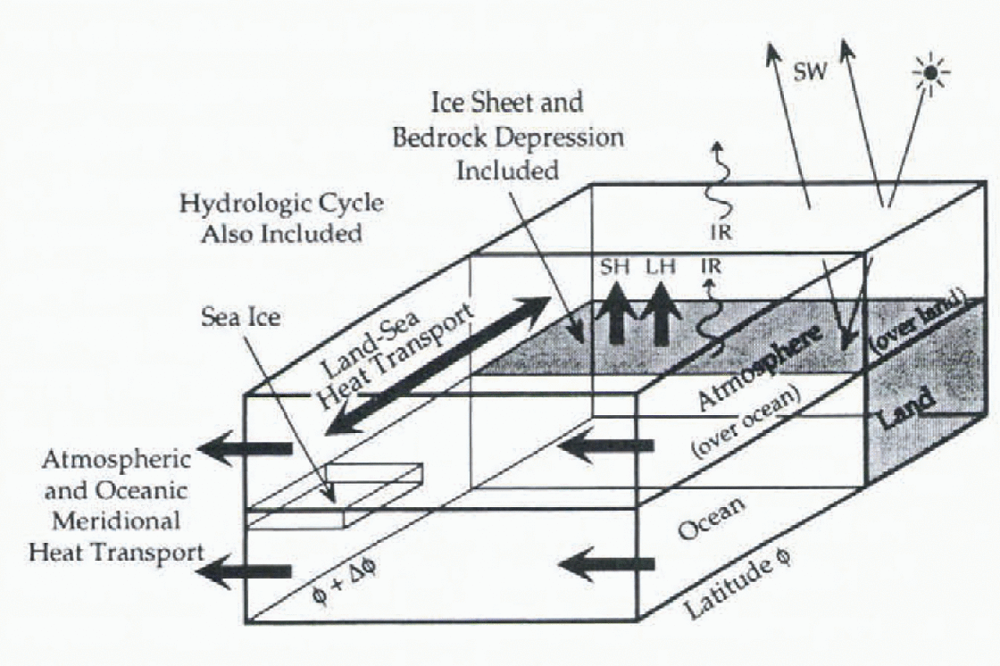
Fig. 1. Schematic diagram of the CCSLI model: schematic of one 10° latitude zone of the atmosphere-ocean-sea-ice-land portions of the model indicating computed and specified vertical and horizontal energy fluxes. SW is solar radiation, IR is infrared radiation, SH is sensible heat flux, and LH is latent heat flux.

The hydrologic cycle (Reference Chu and LedleyChu and Ledley, 1995) is developed from the thermodynamic energy equation, from which the moisture transport through the system is calculated, and a parameterization of zonally averaged precipitation rates that computes precipitation rates resulting from moisture convergence, evaporation-precipitation recycling within a zone, and baroclinic processes.

The sea-ice model (Reference LedleyLedley, 1988, Reference Ledley1991) is a 3-layer thermodynamic model that includes conduction within ice and snow, penetration of solar radiation into the ice, surface-energy balances, a parameterization of leads, and sea-ice transport on the 10° latitudinal grid.

The land ice-sheet/bedrock-depression model, provided by Birchfield (Reference Birchfield, Weertman and LundeBirchfield and others, 1981; Reference Birchfield and GrumbineBirchfield and Grumbine, 1985), is coupled to the climate model by interpolating the 10° latitudinal atmospheric grid to the 0.2° latitudinal ice-sheet grid, and is asynchronously coupled in time in order to preserve the behavior of the ice-sheet as well as to conserve computer resources. This model consists of an ice-sheet flow model, which assumes a zonal ice sheet with viscous flow on top of a lithosphere-asthenosphere Earth response model. Since the large ice sheets identified in the geologic record do not extend equatorward of 40° latitude, the 0.2° ice-sheet grid extends from the poles to 40° latitude. Calving lines are set at 81° N, 40° N, and 65° S; ice sheets that extend poleward of 81°N or equatorward of 40° N and 65° S are calved into the oceans, thus limiting the latitudinal extent of the ice sheets.

Since the details of the climate system at many points on the ice sheet, such as the leading edge, are important to the evolution of the ice sheet, many of the variables of the energy balance climate model are calculated, interpolated, or specified on the 0.2° grid as well as on the 10° atmospheric grid. For example, precipitation, ablation, surface elevation, and temperatures are calculated and lapse rates are specified on the 0.2° grid. In this manner important mechanisms such as albedo changes and lapse-rate effects are included over the ice sheets with a 0.2° resolution.

The Asynchronous Time Coupling

The asynchronous time coupling of the ice-sheel model to the CCSI model is done in two steps. The first step takes advantage of the long time constant of continental ice and bedrock, which requires one long time-step encompassing a number of years, as compared to a 1.09 day time-step required by the CCSI portion of the model for seasonal resolution. The sensitivity (i.e. the difference between a baseline simulation and a simulation using different coupling parameters) of the CCSLI model to taking a long ice-sheet time-step spanning a number of years is explored in the following section. We will identify a time-step length, T _i, that at once preserves the evolution of the ice sheet as it is simulated with synchronous time-steps, and saves computer resources.

The second asynchronous time-coupling step lakes advantage of the quick response time of the climate system to changes in the boundary conditions represented by the ice sheet and continental ice. Here, the net accumulation budget is computed until equilibrium is reached, and then applied to the ice sheet for a number of years, T _NB. This reduces the number of seasonal cycles that the energy-balance climate model needs to simulate. Typically, it takes anywhere from two to eight years for the net budget to achieve equilibrium when new boundary conditions are applied. Meanwhile, the ice-sheet–lithosphere model is run at set intervals, T _i, as determined by the first set of sensitivity studies, computing the flow of the ice sheet and the response of the bedrock.

A typical simulation, using T _i = 14a and T _NB = 5 a, might go as follows: As the simulation starts, the ice-sheet flow rates are calculated. These values are used for the next 14 years, and are applied to the ice sheet each 1.09 day time-step if the atmosphere is activated, or each year if the atmosphere is being extrapolated. Meanwhile, the atmospheric portion of the model is being computed, and the accumulation and ablation results are being applied to the ice sheet. If the net budgets calculated during years 3 and 4 are nearly identical, the equilibrium net budget is then applied to the ice sheet during years 5–9, at which point the atmospheric portion of the model again starts computing the net budget explicitly. A new equilibrium budget is achieved for years 11 and 12 and the atmosphere is again extrapolated, this time for years 13–17. During year 14, new ice-sheet flow rates are computed which are used until year 28. This process continues for however many years are specified. Sensitivity studies have been conducted to determine the number of years each equilibrium net budget may be applied to the ice sheet before a new net budget is calculated (T _NB. These studies are discussed in the following section.

CCSLI Model Sensitivity Studies

Sensitivity of the CCSLI model to the ice-sheet time-step

The first step in asynchronously coupling the continental ice-sheet model to the CCSI model is to increase the time-step taken by the ice-sheel component compared to the atmospheric component of the model. Here, we show the sensitivity of the simulated Northern and Southern Hemisphere ice sheets to the length of the ice-sheet time-step set to 1 month, 10 years, 20 years, and 50 years as compared to using a 5 year ice-sheet time-step, while consistently computing net budget through the seasonal cycle with 1.09 day time-steps every year.

The Northern Hemisphere ice-sheet simulation is initialized with a parabolic ice sheet 3000 m thick at 66°N and reaching from 46° N to 85° N. This ice sheet is out of equilibrium and thus changes dramatically over the 500 year simulation. Figure 2 shows the initial and final (after 500 years of integration) Northern Hemisphere zonally averaged ice-sheet and bedrock profiles, as well as the sensitivity of the CCSLI model simulation after 500 years to the ice-sheet time-step size. The difference in the ice- and land-surface profile after 500 years of simulation using one month, 10, 20, and 50 year ice-sheet time-steps from that simulated with 5year ice-sheet time-steps is shown. The two main features to notice are 1) the decrease in ice-sheet height as the time-step gets longer, and 2) the exaggerated decreases in the surface elevation at the edges of the ice sheet. The errors increase for a longer ice-sheet time-step size. For example, when using T _i = 100 a in a 500 year simulation the ice-sheet thickness difference at 55°N is 1500 m, an order of magnitude greater than for T _i = 50 a, and there is a 4° change in the position of the leading edge. The cause of the ragged difference profile when one month ice-sheet time-steps are used is unclear. The response of the bedrock is similar, but smaller in magnitude.

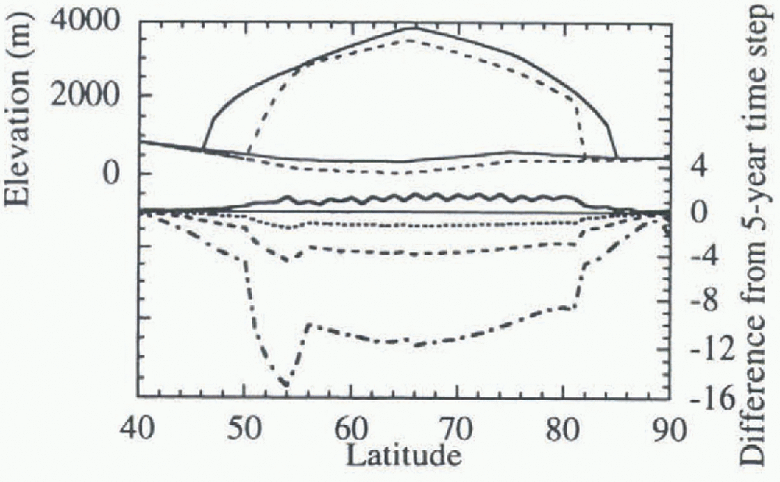
Fig. 2. Ice-sheet time-Step: Northern Hemisphere. Surface elevation and bedrock depression as simulated by the CCSLI model, and change in the surface elevations from the “baseline” for various asynchronous coupling time-steps. The top diagram shows initial ice-sheet conditions (solid lines) and the ice and bedroek configuration after a 500-year simulation (dotted lines); the bottom shows differences for time-steps of 1 mouth (solid lines), 10 years (dotted), 20 years (dashed lines), and 50 years (dot-dashed lines).

The decrease in the ice-sheet height as the time-step gets longer is most likely due to the extrapolation of the initially higher flow rates that were computed for an ice sheet that is larger than its equilibrium size over the long time-step. When shorter time-steps are used the flow rates decrease as the ice sheet gets smaller, thus reducing the magnitude of the decrease in the ice sheet.

The exaggerated decreases in the Northern Hemisphere ice- and land-surface profile at the edges are the result of the relatively large parabolic-shaped ice sheet being used as initial conditions. At the northern edge the ice sheet calves into the Arctic Ocean. At the southern edge the ice sheet is located in a region where there would be extreme ablation under present conditions, so the initial ice sheet is subjected to extreme ablation at that location.

The Southern Hemisphere ice-sheet simulation is initialized with an ice sheet that is 3000m thick at 90° S and extends from the South Pole to 65° S (Fig. 3). This ice sheet is much closer to equilibrium than the Northern Hemisphere ice sheet, and thus there is a much smaller sensitivity, to the ice-sheet time-step size after 500 years (Fig. 3). Most of the sensitivity of the ice/land profile to time-step size after 500 years is <0.5m over an ice sheet that ranges up to 3000m thick, with the largest sensitivity occurring when the 50 year ice-sheel ltime-step is used. It is expected that, as the ice sheet comes closer to equilibrium, the impact of the longer ice-sheet time-step will be reduced.

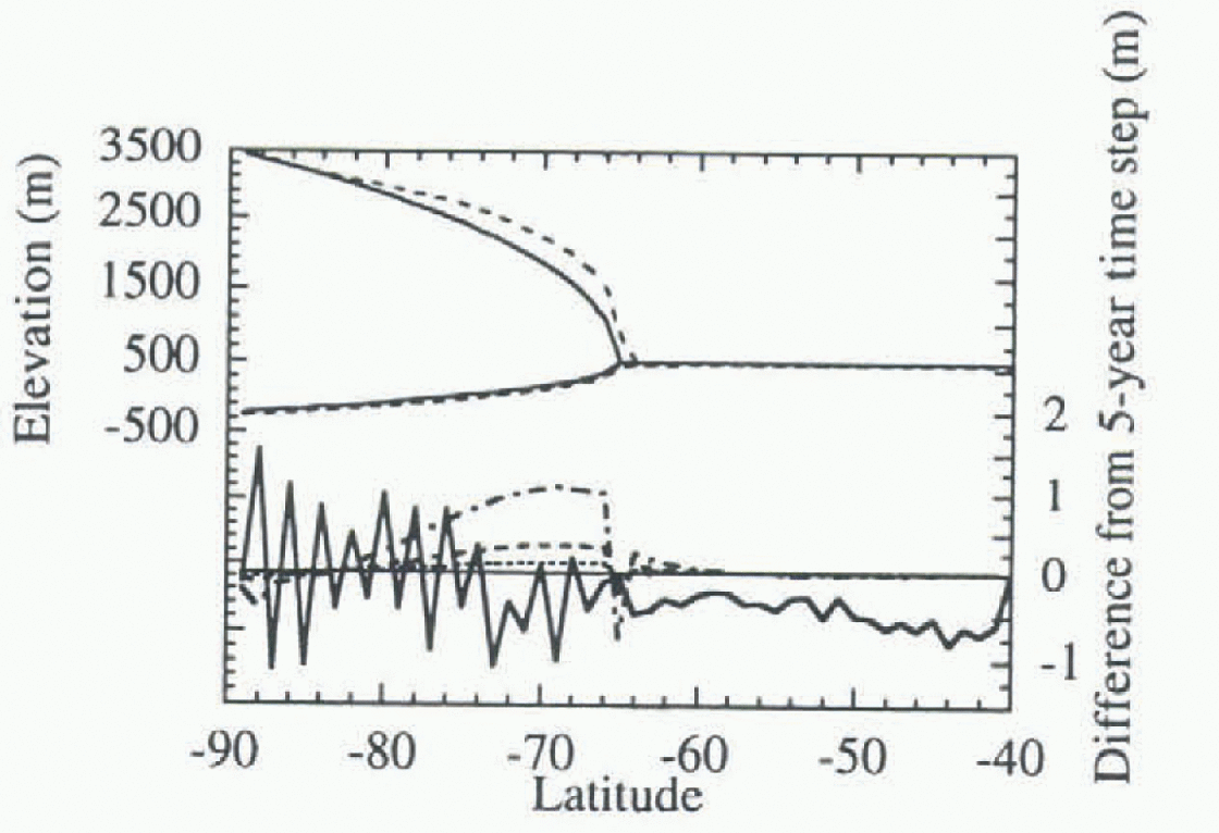
Fig. 3. Ice-sheet time-step: Southern Hemisphere. Surface elevation and bedrock depression as simulated by the CCSLI model, and change in the surface elevations from the “base-line” simulation. The top diagram shows initial ice-sheet conditions (solid lines) and the ice and bedrock configuration after 500 years of model evolution (dotted lines); the bottom shows differences for time-steps of 1 month (solid lines), 10 years (dotted), 20years (dashed lines) and 50 years (dot-dashed lines).

A third simulation examines a Northern Hemisphere ice sheet with accumulation and ablation set to zero (Fig. 4). This simulation isolates the numerical error of the explicit time-stepping scheme used in the ice-sheet model from errors caused by the coupling of the ice-sheet model to the CCSI model. The sensitivity for a 50 year time-step is nearly 1.6 m, in which the ice is 800m thick, and near 1.0 m at the edges. This is the same order of magnitude as the Southern Hemisphere simulation, which is near equilibrium but still an order of magnitude less than the sensitivity in the far-from-equilibrium Northern Hemisphere case. This suggests that much of the sensitivity of the Southern Hemisphere ice sheets to the ice-sheet time-step size is due to limitations in the numerical scheme of the ice sheets and not the coupling of the models.

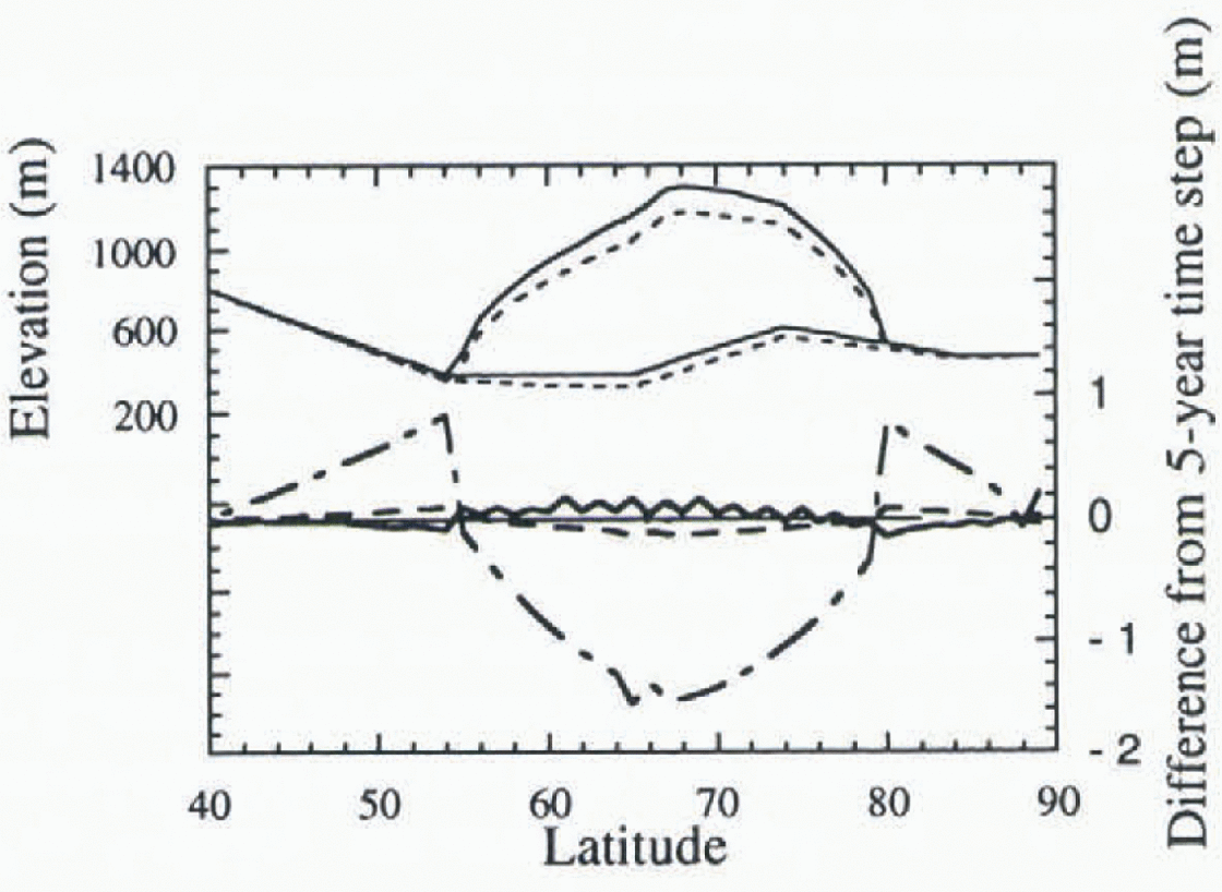
Fig. 4. Ice-sheet time-step: Northern Hemisphere. Surface elevation and bedrock depression after 500 years as simulated by the CCSLI model, and change in the surface from the “baseline” simulation. The top of the diagram shows initial ice-sheet conditions (solid lines) and the ice and bedrock configuration after 500 years of simulation (dotted lines); the bottom shows differences for time-Steps of 1 month (solid lines), 10 years (dotted), and 50 years (dot-dashed lines).

The results suggest that the numerical error introduced by a 10 year ice-sheet time-step is small enough, even when imposed on an initial ice sheet that is significantly out of equilibrium, to justify its use. What is not completely clear from this study is, given the large range of the rate of change of the ice sheets through geologic time, what time-step size is necessary to preserve sufficiently the evolution of the ice sheet simulated. We have examined two extremes here: an ice sheet well out of equilibrium (the Northern Hemisphere); and an ice sheet near equilibrium (the Southern Hemisphere). Further investigation is needed to determine what ice-sheet time-step size will be appropriate for the rate of the natural variation of the ice sheets, but we have placed a lower bound of 10 year time-steps on the problem. Unfortunately, while using a 5 year time-step uses about 10% less CPU time than a synchronous simulation, virtually no additional savings are obtained by using 10 or 50 year time-steps, since the simulation under these conditions is dominated by the computation of the seasonal cycle.

Sensitivity of the CCSLI model to the net budget extrapolation interval

The second step in asynchronously coupling the continental ice-sheet model to the CCSI model is to determine a net accumulation budget to be applied over an extended period, thus reducing the number of seasonal cycles that must be computed with 1.09 day time-steps. Here, three sensitivity studies are described that test the sensitivity of the evolution of an ice sheet to a second asynchronous coupling parameter, T _NB. This parameter determines the number of years an equilibrium net budget may be applied to the ice sheet before the calculation of a new net budget is necessary. A 10 year ice-sheet time-step T _i was used in all three cases.

The first study uses current climatological conditions, i.e. present-day solar radiation, an Antarctic ice sheet that is 3000 m thick at 90°S and extends to 64°S, and no initial Northern Hemisphere ice sheet. (Since this is a zonally averaged model the Greenland ice sheet is ignored in this case.) Note that this is a near-equilibrium scenario in which a single ice sheet is evolving very slowly. Figure 5 shows the sensitivity of the Southern Hemisphere ice-sheet elevations to the application of a net budget for 10 years and 50 years as compared to a synchronous run. Most of the sensitivity after 500 years is <1.0 m over an ice sheet that ranges up to 3000 m thick, although the largest dilferencc is near the leading edge where the ice sheet is thinner (1.0 m out of 400m at 65° S). The greatest sensitivity occurs when the interval over which the net budget is applied is the longest.

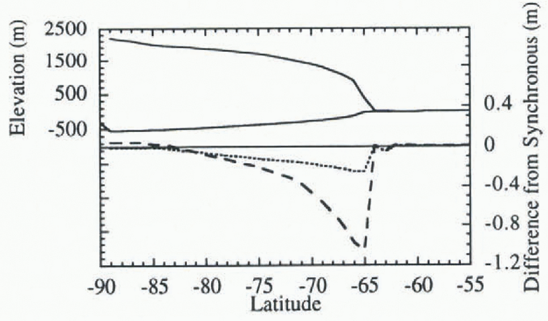
Fig. 5. Extrapolation interval study case 1: near equilibrium. Ice sheet and bedrock configuration in the Southern Hemisphere (solid line) after a 500-year synchronous simulation and change in surface elevation from the synchronous simulation after 500 years when applying the net budget over intervals of 10 years (dotted line) and 50 years (dashed line).

The second case uses current climatological conditions with the exception of an initial Northern Hemisphere ice sheet with a maximum initial thickness of 1000 m at 68°N, and extending from 55° N to 80° N, and no initial bedrock depression. This is a non-equilibrium scenario in that the Northern Hemisphere ice sheet is out of equilibrium in terms of flow, net accumulation, and bedrock response, and changes dramatically over the 500 year simulation. Figure 6 shows the Northern Hemisphere ice sheet/bedrock profile after 500 years of evolution in a synchronous simulation, and the impact on that ice-sheet profile of applying the net budget for 5, 10 and 50 years before it is recomputed. Note that the ice sheet has retreated to around 60° N, and that the ice sheet is still melting rapidly in the region from 60° N–65° N. There is relatively little change in the ice sheet at its northern edge. Most of the sensitivity after 500 years is < 1.0 m over an ice sheet that is about 1000 m thick. The greatest sensitivity in this case occurs at around 65° N when the interval over which the net budget is applied is the longest. The sensitivity, is greatest near the leading-edge, but not directly at it. This is because the ice sheet is so far from equilibrium at the equatorward edge, and large negative net budgets are computed in all cases making the differences between them small.

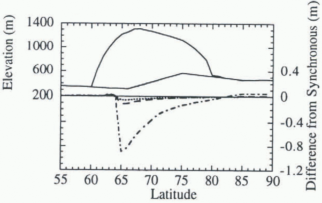
Fig. 6. Extrapolation interval study case 2: far from equilibrium. Ice-sheet and bedrock configuration in the Northern Hemisphere after a 500-year synchronous simulation (solid line) and change in surface elevation from the synchronous simulation after 500 years when applying the net budget over intervals of 5 years (dotted line), 10years (dash-dot line), and 50years (dashedline).

The third case of the sensitivity study is a more realistic non-equilibrium scenario, which uses the solar radiation distribution of 115000 years ago, near the beginning of the most recent ice age. This test is designed to show the sensitivity of the CCSLI model to the asynchronous coupling parameters in an experiment designed to be more realistic, i.e. in which the large-scale features of the climate system are not in equilibrium, but are evolving moderately on decadal time-scales. Figure 7 shows the initiation of a Northern Hemisphere ice sheet over a period of 100 years in a synchronous run, and the sensitivity of the ice-sheet elevations to applying the net budget for 10 and 50 years before recomputing. Most of the sensitivity after 100 years is less than 0.3 m over an ice sheet that is up to 20m thick. The greatest sensitivity in this case occurs near the leading edge of the ice sheet, and when the interval over which the net budget is applied before recalculation is the longest.

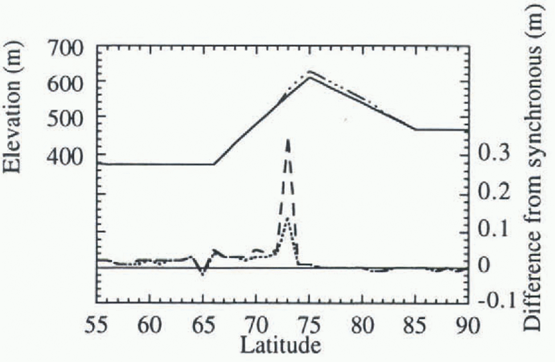
Fig. 7. Extrapolation interval study case 3: moderate evolution. Initial topography and final ice-sheet accumulation after a 100-year synchronous simulation in the Northern Hemisphere and changes from the synchronous simulation when the net budget is applied for 10 years and 50 years. Initial topography (solid line), final ice sheet (dot-dot-dot-dash line), 10 year interval differences (dotted line), and 50 year interval differences (dashed line).

In all three sensitivity study cases the greatest sensitivity was near the leading edge of the ice sheet. Over longer periods of time the leading edge of an evolving ice sheet will advance or retreat and spread this difference over a greater area, thus reducing the relative sensitivity at any given point. In fact the greatest sensitivity did not occur directly at the leading edge in case two, in which the ice sheet was evolving the fastest over the 500 year simulation.

These results suggest that the numerical error introduced by a 10 year application of each equilibrium net accumulation budget before a new net accumulation budget is calculated is small enough, even when imposed on an ice

sheet that is significantly out of equilibrium, to justify its use. These results are generally true for the range of scenarios described here, including an ice sheet near equilibrium, a quickly melting ice sheet, and the early stages of ice-sheet initiation. Also, the small additional error introduced by applying the net budget for 50 years before recomputing, especially when the ice sheel is closer to equilibrium and is thus evolving slowly, may make the use of this interval acceptable in many cases. In fact, further studies with T _NB = 200 a show that the sensitivity in the near-equilibrium case is still only around 6.0 m at the leading edge after 500 years, as compared with 1.0m with T _NB = 50 a, although we would expect differences at the leading edge to be multiplied over longer time periods because of albedo feedbacks or other non-linear affects.

Discussion

The purpose of introducing the asynchronous coupling schemes is to conserve computer time while preserving the integrity of the simulations. The amount of computer time saved in these three cases compared to a synchronous run is greatest for the case with the most slowly evolving ice sheet when it takes fewer years to compute the net budget, but saving are substantial in all cases. While there is a 10% saving in computer time over a synchronous run when using a 10 year ice-sheet time-step T _i (Reference SteenSteen, 1995), applying the net budget for T _NB = 50 a provides an additional saving of 78% for the near-equilibrium case, 75% for the ice-initiation case, and 71 % for the ice-retreat case. Using a 10 year interval for applying each net budget application (T _NB = 10a) gives a saving of 60, 55, and 48% respectively.

Generally it takes between two and eight simulated seasonal cycles for the net budget to reach equilibrium after the previous net budget was applied over the extrapolation interval T _NB of 10–50 years. Each new calculation of the net budget uses the previous equilibrium conditions of the atmosphere as its new initial conditions. When the ice sheet is near equilibrium, each new accumulation budget is nearly the same as the previous one, so fewer calculations are needed to determine the new equilibrium budget and the savings in computer time are largest for this case. When the boundary conditions of an ice sheet change substantially, over an extrapolation interval, the net budget is also further from equilibrium and more calculations are needed to determine each new net budget. Computer efficiency is expected to be greater for slowly evolving ice sheets than for quickly evolving ice sheets, although our sensitivity study shows that savings are substantial for many cases, including for an ice sheet that evolves at a realistic rate.

Using these results, it can he estimated that the simulation of 150 000 years of a glacial cycle will take about 12 supercomputer CPU hours, almost an order of magnitude less than a fully coupled EBM simulation.