


1. Introduction
Considering their sensitivity and as a most direct and apparent visible indicator of regional climate change, Himalayan glaciers have been subjected to numerous studies, from field-based investigations to the modern state-of-the-art remote sensing approach, for more than a century (Bolch and others, Reference Bolch2012; Dobhal and others, Reference Dobhal, Mehta and Srivastava2013; Brun and others, Reference Brun, Berthier, Wagnon, Kääb and Treichler2017; Schmidt and Nüsser, Reference Schmidt and Nüsser2017; Nüsser and Schmidt, Reference Nüsser and Schmidt2021).
Since the 1990s, the advancement in remote sensing and in situ-based glacier monitoring results suggested an accelerated glacier melting and mass loss in the Himalaya and surrounding regions (Pratap and others, Reference Pratap, Dobhal, Bhambri, Mehta and Tewari2016; Brun and others, Reference Brun, Berthier, Wagnon, Kääb and Treichler2017) that has caused a substantial modification of glacial hydrology (Akhtar and others, Reference Akhtar, Ahmad and Booij2008; Nie and others, Reference Nie2021), river runoff and contributed to the ongoing rising sea level (Zemp and others, Reference Zemp2019; Lee and others, Reference Lee2021). Accelerated glacier retreat and surface morphological changes due to ongoing climate warming result in the development of new and expansion of the existing glacial lakes (supraglacial and moraine-dammed) that could be a potential source of glacial lake outburst floods in the Himalaya (Schmidt and others, Reference Schmidt, Nüsser, Baghel and Dame2020; Shugar and others, Reference Shugar2020; Shukla and Sen, Reference Shukla and Sen2021; Kumar and others, Reference Kumar, Mehta and Shukla2021a). However, systematic and quantitative monitoring of the glaciers, viz., field and remotely-sensed based changes in a frontal position (Kumar and others, Reference Kumar, Mehta, Mishra and Trivedi2017, Reference Kumar2021b; Garg and others, Reference Garg2018; Mal and others, Reference Mal, Mehta, Singh, Schickhoff and Bisht2019), mass balance (glaciological and geodetic), debris thickness, and its role in glacier melting (Dobhal and others, Reference Dobhal, Mehta and Srivastava2013; Pratap and others, Reference Pratap, Dobhal, Mehta and Bhambri2015; Bhushan and others, Reference Bhushan, Syed, Arendt, Kulkarni and Sinha2018; Mehta and others, Reference Mehta, Kumar, Garg and Shukla2021), ice thickness and volume (Gantayat and others, Reference Gantayat, Kulkarni and Srinivasan2014; Mishra and others, Reference Mishra, Negi, Banerjee, Nainwal and Shankar2018; Farinotti and others, Reference Farinotti2019), formation and expansion of glacial lakes (Shukla and others, Reference Shukla, Garg and Srivastava2018; King and others, Reference King, Bhattacharya, Bhambri and Bolch2019), surface ice velocity (Tiwari and others, Reference Tiwari, Gupta and Arora2014; Shukla and Garg, Reference Shukla and Garg2020), and fluctuation of equilibrium line altitude (Kayastha and Harrison, Reference Kayastha R and Harrison S2008; Kumar and others, Reference Kumar, Mehta, Shukla, Kumar and Garg2021c), has been done in and around the Himalayan region.
Fieldwork in the Himalayan terrain is challenging due to rugged topography and harsh climatic conditions. Based on field approaches, very few studies have been conducted on the same glacier for long-term monitoring to understand the state of the glacier under ongoing climate change (Azam and others, Reference Azam2016; Dobhal and others, Reference Dobhal, Pratap, Bhambri and Mehta2021; Mehta and others, Reference Mehta, Kumar, Garg and Shukla2021, Reference Mehta, Kumar, Kunmar and Sain2023). Inadequate ice thickness and mass balance data make ice volume estimation extremely difficult for the Himalayan glaciers (GlaThiDa Consortium, 2019; Kumari and others, Reference Kumari2021; Mishra and others, Reference Mishra, Nainwal, Dobhal and Shankar2021). In contrast, understanding the ice thickness and distribution is foremost required for the Himalayan glaciers. However, existing approaches, like remote sensing, cannot directly estimate the glacier thickness. Based on ground penetrating radar, very few studies (only 14 to date) have been carried out on glacier thickness in the Indian Himalaya (Mishra and others, Reference Mishra, Nainwal, Shankar, Pandey, Pandey, Ray, Arora, Jawak and Shukla2022). Therefore, numerous methods and models have been used to estimate the ice thickness distribution and volume of the glaciers in the Himalaya and other regions, e.g. GlaThiDa (Welty and others, Reference Welty2020), the consensus global glacier thickness models (Farinotti and others, Reference Farinotti2019; Millan and others, Reference Millan, Mouginot, Rabatel and Morlighem2022), and regional efforts (e.g. Frey and others, Reference Frey2014). These models are essential without field measurements and can estimate the thickness and volume of a glacier.
In the present study, we used the Himalayan Glacier Thickness Mapper (HIGTHIM) tool, a semi-automated approach based on the laminar flow method (Kulkarni and others, Reference Kulkarni2019, HIGTHIM manual), utilizing the relation between glacier surface velocity and ice thickness (Cuffey and Paterson, Reference Cuffey and Paterson2010; Gantayat and others, Reference Gantayat, Kulkarni and Srinivasan2014). Further, the HIGTHIM tool is used to estimate the depth, water volume of the potential lakes and identify the glacial bed topography for overdeepening sites. Moreover, field observations (2015–2021) and a feature tracking algorithm in COSI-Corr on Landsat data are used to provide recent changes (snout fluctuations, surface morphology, and surface ice velocity). A model-based approach has been carried out over the Parkachik Glacier for the first time.
2. Study area
Parkachik Glacier is one of the largest glacier in the Suru River valley (34°02'N and 76°00'E), covering an area of ~53 km2 and is ~14 km long and northward trending. The glacier originates from the Nun (7135 m a.s.l.) and Kun (7077 m a.s.l.) peaks south of the Suru River. Parkachik Glacier is a valley glacier with four accumulation basins (thus has four flow units), which all feed through icefalls into a glacier tongue of approximately 7 km long and 800 m wide. Moreover, prominent ogives occur over the entire length of the glacier tongue below the icefalls, which makes the glacier surface undulating and prone to supraglacial lake development (Fig. 1). The Suru River valley is a part of the Southern Zanskar Ranges, western Himalaya. The Suru River valley has 252 glaciers covering 11% of the catchment area, and the average annual snowline altitude of the basin is 5011 ± 54 m a.s.l. (Shukla and others, Reference Shukla, Garg, Mehta, Kumar and Shukla2020a). Parkachik Glacier is known by different names, such as ‘Ganri Glacier’ (Toposheet of 1906, Workman and Workman, Reference Workman and Workman1909) and ‘Kangriz Glacier’ (Toposheet of 1962, Garg and others, Reference Garg2018).
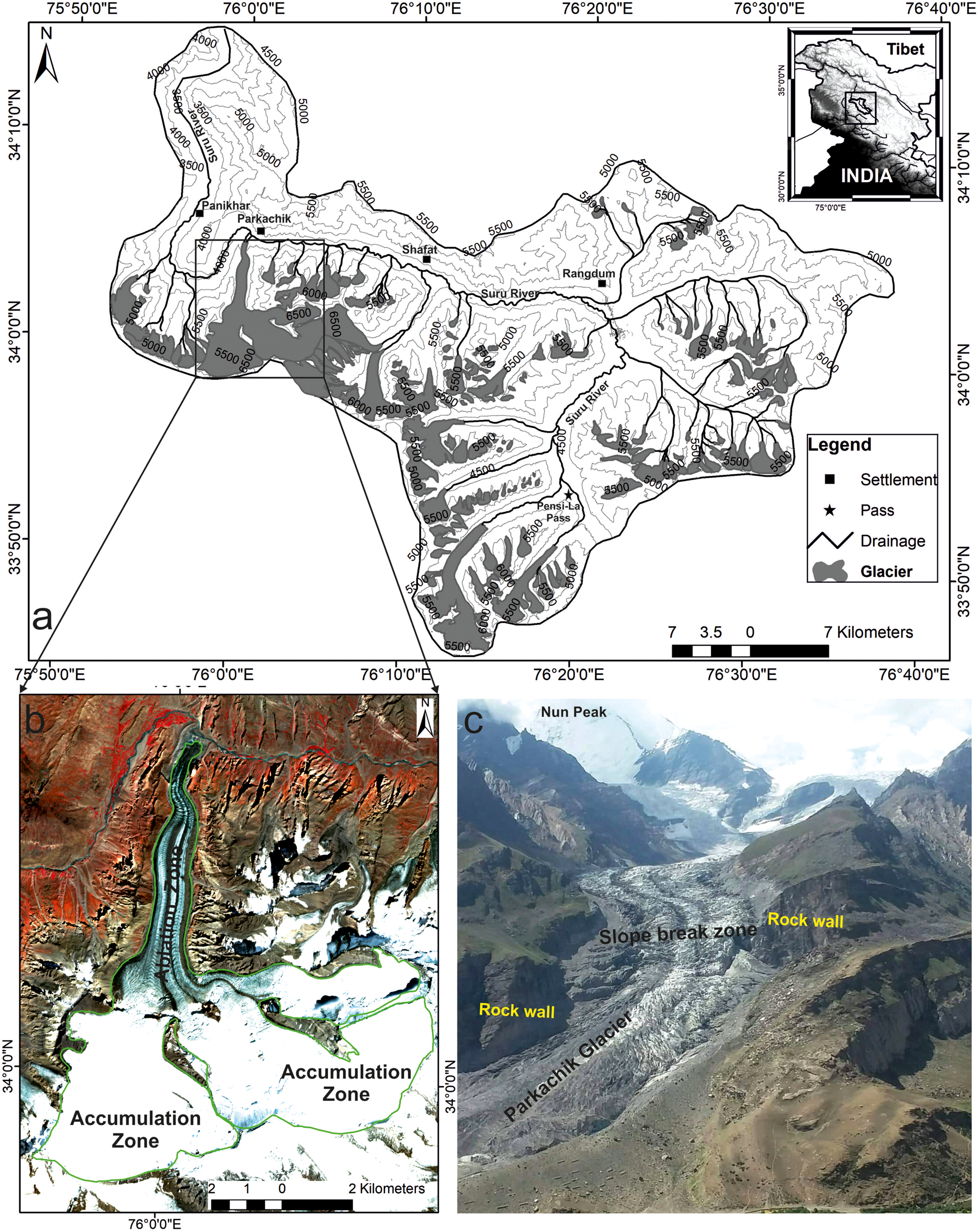
Figure 1. (a) Location of the Suru River basin and Parkachik Glacier (inset). (b) Sentinel-2A (2021) image showing the Parkachik Glacier. (c) A Photograph of the glacier showing geological and geomorphic features on and around the glacier. The glacier outlines and drainage are digitized manually from the Sentinel-2A (2021) image and contour line elevation data from ASTER GDEM (2011).
Parkachik Glacier terminus is dynamic (calving from the west) and has formed several recessional moraines and mounds in the proglacial area (Garg and others, Reference Garg2018, Reference Garg, Shukla, Mehta, Kumar and Shukla2019; Kumar and others, Reference Kumar, Mehta, Shukla, Kumar and Garg2021c). Due to the glacier recession, a proglacial lake was formed after 2015 at ~3600 m a.s.l. on the west part of the terminus and expanded rapidly. Numerous geomorphological (series of lateral, hummocky, and recessional moraines) features are formed in the periphery of the glacier, which suggests that the glacier was very active in the past (2.3 ± 0.2 ka till the present) (Kumar and others, Reference Kumar, Mehta, Shukla, Kumar and Garg2021c). These geomorphological features are evidence of glaciation/deglaciation phases observed from the glacier front (~3650 m a.s.l.) to ~2 km downstream near Parkachik village (3550 m a.s.l.).
The mid-latitude westerlies are the important source of moisture supply to the study area, with a wide variability in snowfall during winters (Kumar and others, Reference Kumar, Mehta, Shukla, Kumar and Garg2021c). The instrumental meteorological data from the study area is not available. However, without meteorological data, Climate Research Unit Time Series (CRU-TS 4.03) data from 1901–2018 have been used to infer the climatic conditions in the study area (Harris and others, Reference Harris, Osborn, Jones and Lister2020; Mehta and others, Reference Mehta, Kumar, Garg and Shukla2021). Mehta and others (Reference Mehta, Kumar, Garg and Shukla2021) suggested that the mean monthly minimum temperature (−10°C) in winter (January) and the average minimum monthly precipitation (11 mm) occurred in November. Further, the maximum monthly mean temperature (18°C) and average precipitation (71 mm) were recorded in summer.
3. Material and methods
3.1. Datasets and pre-processing
In this study, geospatial techniques on multispectral and multi-temporal satellite scenes from CORONA KH-4 (1971), Landsat 7 ETM+ (1999–2000, 2002, and 2009), Operational Land Imager (OLI) (2020–2021), and Sentinel-2A (2021) were used to get the preliminary information of glacier outline and frontal position. Declassified CORONA KH-4 (used for area and length), Landsat and Sentinel-2A imageries (used for area, length, and surface ice velocity), and ASTER (GDEM) were utilized for topographic information, generating contours for input in the HIGTHIM tool (Table 1).
Table 1. Description of datasets used for analysis in this study

First, the acquired satellite images were co-registered by the projective transformation method using the Landsat ETM+ for the year 1999. However, the CORONA KH-4 image subset was co-registered using a two-step approach (i) Projective transformation using 23 ground control points (GCPs) and (ii) Spline adjustment of the subset image (Bhambri and others, Reference Bhambri, Bolch and Chaujar2012). The road intersection and the rocky mountains, convergence of streams and edges were used as GCPs, which were acquired from Landsat ETM+ 1999 images. We adopted the standard image rectification and interpretation procedure as documented by several workers (Goossens and others, Reference Goossens, De Wulf, Gheyle and Bourgeois2006; Bhambri and others, Reference Bhambri, Bolch and Chaujar2012; Chand and Sharma, Reference Chand and Sharma M2015; Shukla and Ali, Reference Shukla and Ali2016; Shukla and Garg, Reference Shukla and Garg2019). After that, the glacier outline was delineated using manual digitization on a standard false color composite (incorporating a standard combination of spectral bands; SWIR-NIR-G). The manual delineation of the glacier boundary is labor extensive, but having a high degree of accuracy is still in practice (Garg and others, Reference Garg, Shukla, Tiwari and Jasrotia2017; Kaushik and others, Reference Kaushik, Joshi and Singh2019). Further, the extracted glacier boundary for the year 2021 was used to estimate the ice thickness distribution. Moreover, the length changes of the glacier were quantified using the parallel line method for which collateral strips spaced at an 80 m distance were drawn between the two glacier outlines (Schmidt and Nüsser, Reference Schmidt and Nüsser2009). The average distance of these collateral strips was considered to be the total frontal retreat of the Parkachik Glacier. In addition, the glacier boundary and frontal position extracted from the satellite data were validated during the field.
3.2. Glacier survey
Fieldwork has been carried out on the Parkachik Glacier since 2015 using a differential global positioning system; changes in frontal position and area have been monitored annually with the help of ground control points taken (stable boulders from right, left, and center) with an accuracy of <1 cm near the glacier front (see Fig. 4). Further, the in situ measurements of glacier surface lowering, debris thickness, and frontal changes were observed from 2015 to 2021. The distance from these reference stations (to the glacier snout) was measured using a measuring tape up to the glacier base from the snout's left, right and center. Average length change was calculated based on the average recession of the glacier from left, right, and center parts for every studied year. The field-based monitoring of the glacier recession and area change was done following the methods given in our recent studies (Kumar and others, Reference Kumar, Mehta, Mishra and Trivedi2017; Mehta and others, Reference Mehta, Kumar, Garg and Shukla2021, Reference Mehta, Kumar, Kunmar and Sain2023). In addition, several features representing higher glacier melting, e.g. supraglacial ponds, ice cliffs, and patchy debris cover (thin and thick), were observed.
3.3. Surface ice velocity
The surface ice velocity was calculated using the optical image correlation technique from repeated Landsat images for two consecutive years (1999–2000 and 2020–2021). The method is based on the Co-registration of Optically Sensed Images and Correlation (COSI-Corr) software, which is a free plug-in module integrated into ENVI that provides tools to accurately orthorectify, co-register, and correlate the remotely sensed images developed by (Leprince and others, Reference Leprince, Ayoub, Klinger and Avouac2007), and described in detail by Scherler and others (Reference Scherler, Leprince and Strecker2008). COSI-Corr uses a Fourier-based highly advanced matching program that offers sub-pixel accuracy and is widely used to measure glacier movements (Heid, Reference Heid2011; Shukla and Garg, Reference Shukla and Garg2020). Its algorithm works on single-band grayscale images (Das and Sharma, Reference Das and Sharma2021).
This study used the panchromatic band of Landsat 8 OLI, 15 m resolution of wavelength 0.50–0.66 μm, and Landsat ETM+ panchromatic (0.52–0.90 μm) 15 m. The frequency correlation function is employed to get East–West (EW) and North–South (NS) displacements images along with a signal-to-noise ratio (SNR) image. The initial and final window size combination for frequency correlation was set at 64 and 32 pixels, respectively, and the step was set as 2 pixels resulting in a ground resolution of 30 m. The frequency mask threshold and robustness iteration was set as 0.9 and 2, respectively, to reduce the effect of noise on the displacement correlation map. These parameters were chosen based on previous studies on Himalayan glaciers (Gantayat and others, Reference Gantayat, Kulkarni and Srinivasan2014; Sattar and others, Reference Sattar, Goswami, Kulkarni and Das2019; Shukla and Garg, Reference Shukla and Garg2020; Das and Sharma, Reference Das and Sharma2021; Kulkarni and others, Reference Kulkarni, Prasad and Shirsat2021). Further, post-processing was done to correct potential biases by removing all pixels having SNR <0.9 to discard poorly correlated pixels. After removing erroneous pixels, the resultant displacement was calculated using the Euclidean distance geometry formula.

Where D is total displacement, x is the East–West and y is North–South displacement.
The acquisition time between the two images (t days) was then used to compute the ice velocity (V) in m d−1, which was normalized to annual velocities for 365-day intervals (m a−1).

3.4. Ice thickness estimation
The ice thickness was estimated by the Himalayan Glacier Thickness Mapper (HIGTHIM) tool (Kulkarni and others, Reference Kulkarni2019, HIGTHIM manual). The tool was developed based on the laminar flow equation (Eqn 3) and used in recent studies where ice thickness data are unavailable (Gopika and others, Reference Gopika, Kulkarni, Prasad, Srinivasalu and Raman2021; Singh and others, Reference Singh2023). The glacier boundary, flowlines, moraines, contour polygons in vector format, digital elevation model (DEM) and glacier surface ice velocity in raster format were given as input in the HIGTHIM tool. The glacier thickness, bed topography, and overdeepening sites in the glacier are the output of the HIGTHIM tool. In HIGTHIM, ice thickness is estimated from the laminar flow and basal shear stress equation (8.5) given by Cuffey and Paterson (Reference Cuffey and Paterson2010). The laminar flow equation for estimating ice thickness is widely used on the Himalayan glaciers (Gantayat and others, Reference Gantayat, Kulkarni and Srinivasan2014; Maanya and others, Reference Maanya, Kulkarni, Tiwari, Bhar and Srinivasan2016; Remya and others, Reference Remya, Kulkarni, Pradeep and Shrestha2019; Sattar and others, Reference Sattar, Goswami, Kulkarni and Das2019; Gopika and others, Reference Gopika, Kulkarni, Prasad, Srinivasalu and Raman2021).

Where H is ice thickness in meters, U S is surface ice velocity derived from COSI-Corr, ρ is the density of ice assigned a constant value of 900 kg m–3, g is the acceleration due to gravity (9.8 m s−2), A is a creep parameter (which depends on temperature, fabric, grain size, and impurity content), assigned a value of 3.24 × 10⁻²⁴ Pa−3 s−2 for temperate glaciers (Cuffey and Paterson, Reference Cuffey and Paterson2010), and ƒ is shape factor with a constant value 0.8 in the HIGTHIM, i.e. the ratio between the driving stress and basal stress along a glacier (Haeberli and Hoelzle, Reference Haeberli and Hoelzle1995), α is slope estimated from ASTER (GDEM) contours at 100 m intervals.
The ice thickness estimates were obtained by manually digitized flowlines (Linsbauer and others, Reference Linsbauer, Paul and Haeberli2012; Gantayat and others, Reference Gantayat, Kulkarni, Srinivasan and Schmeits2017), and depending upon the size and shape of a glacier, multiple flowlines can exist Pieczonka and others (Reference Pieczonka, Bolch, Kröhnert, Peters and Liu2018). The flowlines were interpolated over the entire glacier area to get a U-shaped glacier thickness distribution, assuming zero ice thickness along the ice margins (Sattar and others, Reference Sattar, Goswami, Kulkarni and Das2019). Therefore, if more than one flowline exists, the flowlines are delineated at a 150 m distance from the glacier margin to 300–400 m from each other to achieve ideal results (Kulkarni and others, Reference Kulkarni2019; HIGTHIM manual). We draw seven flowlines over the Parkachik Glacier. Further, for the remaining pixels, the spline interpolation technique was used with the boundary condition that ice thickness is maximum along the center flowlines and zero at glacier margins; this gives a complete spatial distribution of glacier depth (Kulkarni and others, Reference Kulkarni, Prasad and Shirsat2021).
3.5. Uncertainty estimation
The study is based on several multi-satellite data of variable resolution and specifications; therefore, it is liable to introduce errors (Paul and others, Reference Paul2013). Various errors can be generated from different sources while estimating glacial frontal retreat and other parameters using remote sensing data such as pre-processing, processing, locational/positional, interpretation, and data quality (Racoviteanu and others, Reference Racoviteanu, Arnaud, Williams and Ordoñez2008, Reference Racoviteanu, Paul, Raup, Khalsa and Armstrong2009). Therefore, different methods were used to estimate errors induced by the above sources as no common consent between glaciologists is reached for error estimation (Hall and others, Reference Hall, Bayr, Schöner, Bindschadlerd and Chiene2003; Basnett and others, Reference Basnett, Kulkarni and Bolch2013; Shukla and Qadir, Reference Shukla and Qadir2016).
Glacier frontal change uncertainty was estimated using the formula given by Hall and others (Reference Hall, Bayr, Schöner, Bindschadlerd and Chiene2003), which was widely used in glacier studies (Shukla and Qadir, Reference Shukla and Qadir2016; Kumar and others, Reference Kumar, Mehta and Shukla2021a)

Where Ut is terminus uncertainty, ‘x1’ and ‘x2’ are the pixel resolution of images 1 and 2, respectively, and ‘σ’ is the registration error (Table 2).
Table 2. Uncertainty in terminus position change estimated as per Hall and others (Reference Hall, Bayr, Schöner, Bindschadlerd and Chiene2003), using Eqn 4

Surface ice velocity derived from COSI-Corr-based feature tracking is prone to various errors derived due to orthorectification, substandard image contrast, and poor image correlation (Sahu and Gupta, Reference Sahu and Gupta2019). Landsat scenes were used for velocity determination, with minimum snow and cloud cover. The cloud-free or <10% cloud cover images were used to minimize the error due to substandard image quality, and ablation zone velocity is considered for glacier dynamics comparative analysis. Image correlation error is minimized by discarding the SNR <0.9.
Velocity error is estimated using the method suggested by (Scherler and others, Reference Scherler, Leprince and Strecker2008), and used in other studies (Garg and others, Reference Garg, Shukla, Garg, Yousuf and Shukla2022b). Ideally, stable terrain conditions surrounding the glacier should be zero. Velocity error in the stable terrain was calculated based on (Berthier and others, Reference Berthier, Raup and Scambos2003) formula. The CNES/Airbus imagery from Google Earth was used to visually outline the stable terrain. The velocity maps from 1999–2000 and 2020–2021 were utilized as a base map to digitize the stable terrain in the ARC-GIS.

Where σoff is the velocity error, SD is the std dev. in the mean velocity of stable terrain, and M stable is the mean velocity of stable terrain. The uncertainty in velocity estimates is calculated for 1999–2000 as M stable 0.46, SDstable 1.32, and uncertainty is 1.78, whereas for the year 2020–2021, it is M stable 0.28, SDstable 0.52, and uncertainty is 0.80.
Moreover, the uncertainty in glacier thickness estimation depends upon various factors, e.g. surface ice velocity, error in slope determination, shape, and density variation. The combined uncertainty in glacier thickness estimates (based on Eqn. 3) is calculated using the expression below.

Where dH is an error in estimated thickness, dUS is the change observed in COSI-Corr-based derived surface ice velocity, glacier shape factor (ƒ) ranged between 0.7 in ablation and 0.9 in accumulation zones (Haeberli and Hoelzle, Reference Haeberli and Hoelzle1995; Linsbauer and others, Reference Linsbauer, Paul and Haeberli2012), dƒ is uncertainty in shape factor, dρ is an error in ice density, and dsinα is uncertainty due to the DEM. The uncertainty in surface ice velocity comes due to orthorectification error, misregistration between the images, and limitations of the COSI-Corr correlation technique (Maanya and others, Reference Maanya, Kulkarni, Tiwari, Bhar and Srinivasan2016; Sattar and others, Reference Sattar, Goswami, Kulkarni and Das2019). Co-registration accuracy of 5 m for Landsat imagery is taken from Gopika and others (Reference Gopika, Kulkarni, Prasad, Srinivasalu and Raman2021), and COSI-Corr accuracy for correlation is in the order of ~1/20th of a pixel or 1.5 m (Leprince and others, Reference Leprince, Ayoub, Klinger and Avouac2007).
No field-based velocity data for the glaciers from this region are available to validate the velocity estimates. The estimated mean velocity of 0.80 m a−1 on the stable ground by the COSI-Corr method is considered an error. The combined velocity error is calculated as 5 m a−1. Considering the typical variation in ice density from 830 to 923 (kg m−3), ±10% uncertainty in ice density is considered, as suggested by Bhambri and others (Reference Bhambri, Mehta, Dobhal and Gupta2015) and Remya and others (Reference Remya, Kulkarni, Pradeep and Shrestha2019). The shape factor varies with ±0.1, giving a relative uncertainty of (12.5%) (Gantayat and others, Reference Gantayat, Kulkarni and Srinivasan2014; Maanya and others, Reference Maanya, Kulkarni, Tiwari, Bhar and Srinivasan2016). The uncertainty in slope estimation arises from DEM vertical inaccuracy. Fujita and others (Reference Fujita, Suzuki, Nuimura and Sakai2008) reported an 11 m vertical inaccuracy for ASTER DEM in the Bhutan Himalayan region. Due to the topographical similarity, similar vertical inaccuracy is considered, and ±9% uncertainty for the sinα value is estimated. A combined uncertainty of ±14.68% was calculated. Further, the uncertainty of ±6.5% in ice thickness arises due to the interpolation algorithm taken from Hutchinson (Reference Hutchinson2011). Therefore, the overall HIGTHIM tool estimated ice thickness uncertainty is ±16%.
4. Results
4.1. Frontal retreat and morphological changes
The glacier has a sudden change in slope (approximately 1.5 km upstream from the glacier terminus) in the lower (~16°) and upper ablation zone (9°). Due to the variability in slope, the glacier retreat is oscillatory.
Overall the glacier retreated by −210 ± 88 m with an average rate of 4 ± 1 m a−1 between 1971 and 2021. The snout of the Parkachik Glacier indicates different fluctuation patterns in various sectors (Fig. 2). Based on the satellite data, the glacier retreat is calculated in 1971–1999 and 1999–2021. The overall retreat of the glacier between 1971 and 1999 was −54 ± 18 m with an average rate of 2 ± 0.6 m a−1. Whereas, between 1999 and 2021, the glacier retreated −246 ± 62 m with an average rate of 12 ± 3 m a−1. Moreover, an advance of the snout of approximately 44 ± 29 m with an average rate of 15 ± 10 m a−1 was observed between 1999 and 2002. This may result from subglacial cavity collapse resulting in a lateral spread of ice and disintegration of the marginal zone. It has also been observed that the glacier snout broke down and blocked the glacier stream for an unknown duration and formed a temporary lake beneath the glacier in 2017 (Fig. 3a). After a few hours, that lake breached, and the broken ice blocks spread around the proglacial area (Fig. 3b). This was observed in the field (2017) discharge data (Fig. 3c), when the emerging stream from the glacier suddenly disappeared for an hour followed by an outburst flood scattering about ice blocks up to ~200 m downstream of the ice margin.

Figure 2. Satellite images of different years showing the glacier margin. (a) CORONA KH-4 image, 1971, (b) Landsat ETM+, 1999, (c) Landsat ETM+, 2002, (d) Landsat ETM+, 2009, (e) Sentinel-2A, 2021. (f) Overall margin fluctuations from 1971 to 2021.

Figure 3. (a) And (b) are the field photographs showing the blocked stream and broken ice blocks after the outburst flood. (c) Field discharge data showing suddenly low and high peaks (red circle) in a discharge after the block and release of energy (Fig. c is modified after Garg and others, Reference Garg2018). The spread ice blocks are clearly shown in Figure b.
Similarly, the field observations from 2015 to 2021 show that the glacier retreated by −123 ± 72 m at an average rate of −20.5 ± 12 m a−1. The left part of the glacier showed a higher retreat of −254 ± 150 m, whereas the right part was quasi-stagnant and retreated only −26 ± 13 m between 2015 and 2021. After 2015 it was observed (in the field) that the glacier front is continuously breaking, and ice-collapsing events are happening regularly. This increased the disintegration and frontal lowering of the glacier between 2015 and 2021. Moreover, the glacier surface (from terminus to upper ablation zone) between 3650 and 3800 m a.s.l. was covered with supraglacial debris of variable thickness (<1 cm to >1 m) and with sediment sizes varying from silts and sand to large boulders exceeding several meters. This variable debris thickness also plays a critical role in glacier melting (Dobhal and others, Reference Dobhal, Mehta and Srivastava2013; Mehta and others, Reference Mehta, Kumar, Garg and Shukla2021, Reference Mehta, Kumar, Kunmar and Sain2023). The details about the glacier retreat and morphological changes are given in Table 3 and Fig. 4.
Table 3. Frontal retreat of the glacier calculated using satellite data and field observations over the past five decades


Figure 4. Field photographs (a to d) from 2015, 2017, 2019, and 2021 (two years intervals), showing the panoramic view of the glacier front and lower ablation zone that was divided into three parts, i.e. left, centre, and right (shown in photo a). (a) Is also showing slope break zone, lateral moraines (light pink color lines), red arrows indicating the changes observed between 2015 and 2021, and yellow circles highlighting the ground control points (stable boulders) taken as reference points for frontal (retreat) monitoring. (a) Showing the location of the proglacial (pgl) lake formed at the left of the glacier terminus.
4.2. Frontal area loss
The frontal area loss was calculated over the same time intervals (1971–2021) as the recession was calculated, and within this period, the rates were variable but accelerated after the year 2009 (Table 4). Further, field evidence revealed that an ice cave was formed at the left portion of the glacier snout (present in 2015) that collapsed (in 2018) could be a probable reason for the enhanced retreat and area loss of the left flank (Fig. 5).
Table 4. Frontal area loss by the glacier between 1971 and 2021


Figure 5. (a) And (b) Field photos (2015 and 2018) show both calving, collapse, and general thinning of the glacier front. The orange boxes show an ice cave present in 2015 and collapsed in 2018. The yellow circle in both photos shows the reference boulders (~4 m in length) for change detection.
4.3. Surface ice velocity
The surface ice velocity of the Parkachik Glacier was computed for the years 1999–2000 and 2020–2021. The overall trend of decreasing glacier velocity was found in 2020–2021 compared to 1999–2000. Only ablation zone velocity estimates were considered for comparative study due to poor image contrast in the accumulation zone, leading to erroneous velocities due to data voids. The velocity over the lower ablation zone during 1999–2000 was estimated to be 45.18 ± 1.78 m a−1 which was reduced to 32.28 ± 0.80 m a−1 between 2020 and 2021. The velocity trends were observed based on three flowlines drawn on the left, central, and right parts of the glacier ablation zone (Fig. 6). The results show a similar overall trend in all flowlines (Fig. 7). Further, the recent velocity of 2020–2021 was correlated with NASA ITS_LIVE velocity extracted from (https://its-live.jpl.nasa.gov/). The present study velocity estimates show a positive correlation (R: 0.80) with the ITS_LIVE velocity (Fig. 8). However, we have considered only those velocities for comparative analysis which were derived from Landsat 8 images having the temporal resolution of 345–370 days between image-pairs.

Figure 6. Surface ice velocity for 1999–2000 and 2020–2021. The red dots are the points taken to compare the present study velocity estimates with the ITS_LIVE velocity.

Figure 7. Surface ice velocity of the glacier left, central, and right parts in 1999–2000 and 2020–2021.

Figure 8. Present study velocity estimates show a positive correlation (R: 0.80) compared to the ITS_LIVE velocity.
An anomalous behavior (advancement) of the glacier between 1999 and 2002 can be understood with abnormal velocity change at the terminus. The glacier terminus showed high velocity from 1999 to 2000 compared to other parts of the glacier, whereas in the slope break zone (3950 m a.s.l.) sudden drop in velocity is seen compared to 2020–2021. The terminus region may be influenced by a proglacial lake or subglacial drainage that might collapse in 1999–2000, increasing the terminus velocity. This suggests that the glacial advancement of 1999–2002 is related to the abnormal velocity in the lower (at terminus) and upper ablation (slope break) zones.
4.4. Ice thickness and overdeepenings
The average ice thickness of the Parkachik Glacier was estimated to be 115 ± 16 m. The thickness of the glacier varies from the terminus to the accumulation zone. Figure 9 clearly shows the variability in ice thickness as it is lower (~44 to 83 m) at the terminus, between 200 and 350 m in the upper ablation zone, and reaches ~441 m in the accumulation zone; however, these estimates needs to be verified by ground-based measurements. Here, we have compared the present study thickness estimates with the global dataset of Farinotti and others (Reference Farinotti2019). The present study estimated the average ice thickness of 115 ± 18 m with a maximum thickness of 441 m, whereas Farinotti and others (Reference Farinotti2019) average thickness was 135 m showing a maximum of 382 m. Such differences arise as thickness estimates were derived from different models and input datasets, including the glacier outline. The most significant differences in glacier thickness are found along the glacier boundaries, where the present study shows lower thickness estimates than Farinotti and others (Reference Farinotti2019), and in the deepest parts of the glacier (Fig. 10).

Figure 9. Modelled (a) ice thickness of the glacier varying from ~44 to 83 m near the terminus, between 200 and 350 m in the upper ablation zone, and reaching >400 m in the accumulation zone. Maximum thickness is modelled as 440 m.

Figure 10. Comparison of the present study thickness estimates with the freely available dataset of Farinotti and others (Reference Farinotti2019). Ice thickness was compared for the three sections (A–B, C–D, and DE). Significant changes in glacier thickness are found along the glacier margin, where the present study shows fewer thickness estimates than Farinotti and others (Reference Farinotti2019).
We have identified three potential overdeepening sites for lake formation on the glacier at different elevations (from lower to upper ablation zone) with a mean depth of 34 to 84 m. However, the expansion and reduction of these lakes depend on the dynamics of the glacier. The estimated future lake depth, area, and water volume are given in Table 5 and Fig. 11.
Table 5. Calculated overdeepenings for future lake development with lake area, mean depth, and water volume


Figure 11. Overdeepenings under the glacier with predicted lake sites (a, b, and c) with depths varying from 20 to 223 m.
5. Discussion
The glaciers in the Suru River valley are generally characterized by their geographical position covering two major ranges, i.e. the Great Himalayan Range and Ladakh Range, at high altitudes, their large size, and the dominance of partially debris-covered ice. The recent glacier inventory of the Suru Basin has suggested a heterogeneity in glacier response (Shukla and others, Reference Shukla, Garg, Mehta, Kumar and Shukla2020a, Reference Shukla, Garg, Kumar, Mehta, Shukla, Dimri, Bookhagen, Stoffel and Yasunari2020b). Shukla and others (Reference Shukla, Garg, Mehta, Kumar and Shukla2020a) reported the overall average retreat rate of the glaciers was 4.3 ± 1.02 m a−1 between 1971 and 2017. Kamp and others (Reference Kamp, Byrne and Bolch2011) suggested a retreat of ~13 m a−1 and a re-advancement of 17 m a−1 for the years 1979–1990 and 1990–1999 of the Parkachik Glacier. Rai and others (Reference Rai, Nathawat and Mohan2013) reported a retreat of 1300 m with an average of 33 m a−1 between 1962 and 2001 of the glaciers in the Doda Basin, Zanskar and Jammu & Kashmir region. Schmidt and Nüsser (Reference Schmidt and Nüsser2017) reported a retreat of 248 m with an average of 5.3 m a−1 between 1969 and 2002 in the Central Ladakh Range. Similarly, the overall frontal recession (4 ± 1 m a−1 between 1971 and 2021) of the glacier reported in this study is consistent with the other studies across the northwest Himalaya (Murtaza and Romshoo, Reference Murtaza and Romshoo2017; Shukla and others, Reference Shukla, Ali, Hasan and Romshoo2017; Mir and Majeed, Reference Mir and Majeed2018; Rashid and Majeed, Reference Rashid and Majeed2018; Shukla and Garg, Reference Shukla and Garg2019; Mehta and others, Reference Mehta, Kumar, Garg and Shukla2021). However, the recent retreat rate (−20 ± 12 m a−1, since 2015) derived from the field survey is higher than other regional studies (Bahuguna and others, Reference Bahuguna2014; Ghosh and others, Reference Ghosh, Pandey, Nathawat and Bahuguna2014; Rashid and Majeed, Reference Rashid and Majeed2018). The accelerated glacier retreat after 2015 in this study suggests the influence of the proglacial lake and the disintegration of the marginal zone of the Parkachik Glacier. Mir and Majeed (Reference Mir and Majeed2018) suggested that the Parkachik Glacier retreated 127 m at a rate of 2.9 m a−1 between 1971 and 2015, which is underestimated, whereas Garg and others (Reference Garg, Shukla, Garg, Yousuf and Shukla2022b) overestimated the glacier recession and reported an overall recession of 497 ± 32 m with an average retreat of 11 ± 0.7 m a−1 between 1971 and 2018. This discrepancy in a recession may largely be ascribed due to the difference in the time frame, resolution of data, field observations (GCPs) and validation, and methodology used for inferring the changes.
Further, the surface ice velocity estimation in this study suggests a slowing down which is primarily due to down wasting and deglaciation, resulting in an increase of debris cover on the glacier surface (ablation zone) and an insufficient supply of snow in the accumulation zone over the past two decades (Garg and others, Reference Garg, Shukla, Tiwari and Jasrotia2017; Shukla and Garg, Reference Shukla and Garg2019; Garg and others, Reference Garg2022a, Reference Garg, Shukla, Garg, Yousuf and Shukla2020b). However, the higher velocity transfer more mass down the glacier, compensating for the glacier recession (Tiwari and others, Reference Tiwari, Gupta and Arora2014; Shukla and Garg, Reference Shukla and Garg2019).
Maanya and others (Reference Maanya, Kulkarni, Tiwari, Bhar and Srinivasan2016) estimated the ice thickness of the Durung-Drung Glacier, one of the largest glaciers in Doda Basin, Zanskar (~63 km from the Parkachik Glacier) derived from the laminar flow equation (Eqn 3) as 100 m at the terminus and 50–400 m in the accumulation zone. Moreover, they identified three potential lake sites with mean depths varying between 40 and 75 m. Similarly, a recent study carried out on Durung-Drung Glacier reported the ice thickness of the glacier between 1 and 311 m with a mean thickness of 155 using the GlabTop (Glacier-bed Topography) model (Rashid and Majeed, Reference Rashid and Majeed2018). In addition, Rashid and Majeed (Reference Rashid and Majeed2018) speculated the formation of 76 potential lakes with varying depths between 7 and 222 m, which is more than the estimates of Maanya and others (Reference Maanya, Kulkarni, Tiwari, Bhar and Srinivasan2016). In this study, the maximum thickness was estimated to be ~441 m in the upper reaches, 350–440 at the center, and 44–80 m at the terminus of the Parkachik Glacier. Rashid and Majeed (Reference Rashid and Majeed2018) suggested that the Durung-Drung could be a suitable glacier for extracting an ice core because of its location in a cold arid climate with an ice thickness of >300 m in the accumulation zone. Similarly, after estimating the thickness of the Parkachik Glacier, we can speculate that the glacier can be a better site for ice core drilling as its estimated maximum depth (441 m) is more than the Durung-Drung Glacier. Although the thickness and overdeepenings site data from this region is very scarce, comparing the present study estimates with the recent studies (Maanya and others, Reference Maanya, Kulkarni, Tiwari, Bhar and Srinivasan2016; Rashid and Majeed, Reference Rashid and Majeed2018) suggests that this study is consistent with other studies in the region and provides credible information about the ice thickness and probability of development of glacial lakes at different sites.
6. Conclusion
In this study, we analyzed multiple glacier parameters (frontal area, glacier thickness, surface ice velocity, bed overdeepenings, and morphological changes) for the Parkachik Glacier, western Himalaya.
We have estimated the ice thickness for Parkachik Glacier from surface velocities and slopes using the laminar flow equation (Eqn 3). The surface velocity slowed down from 45 to 32 m a−1 over the past two decades (1999–2021). The ice thickness attained a maximum value of 441 m in the upper reaches, a range of 350–440 m was found in the middle, and the lower reaches, the range was 44–80 m. Further, using surface ice velocity and slopes, along with basal shear stress and the laminar flow equation, glacier thickness and bed topography were estimated. We identified three potential overdeepening sites for lake formation on the glacier at different elevations (from lower to upper ablation zone) with a mean depth of 34 to 84 m.
Overall the glacier retreat varied between 1971 and 2021. The glacier retreated with an average rate of 2 ± 0.6 m a−1 between 1971 and 1999. Whereas between 1999 and 2021, the glacier retreated at an average rate of 12 ± 3 m a−1. Similarly, the field observations suggest that the glacier retreated at a higher rate of −20.5 ± 12 m a−1 between 2015 and 2021. The field and satellite-based observations indicate that the calving nature of the glacier margin and the development of a proglacial lake may have enhanced the retreat of the Parckachik Glacier. The significant slowdown, extensive surface lowering, progressive growth and expansion of the proglacial lake at the terminus, and consecutive calving of the snout since 2015 suggest accelerated glacier demise.
The comparison of the modelled ice thickness in this study with the other studies (Farinotti and others, Reference Farinotti2017; Sattar and others, Reference Sattar, Goswami, Kulkarni and Das2019) shows that the method is well suited to estimate the ice thickness of the glacier in the region. The Ice Thickness Models Intercomparison eXperiment (ITMIX1) concluded the comparison between various models, as the most reasonable ice thickness estimate can be derived by averaging multiple models. In contrast, the analyses conducted in ITMIX2 do not reveal a singularly superior model among the various models evaluated. However, the Tasman Glacier (valley glacier) Gantayat model was highly reliable and efficient. Also, the small model bias in the Gantayat model is comparable to other thickness models that revealed its performance (Farinotti and others, Reference Farinotti2017; Sattar and others, Reference Sattar, Goswami, Kulkarni and Das2019). Whereas the HIGTHIM used in this study was considered a simple tool in which the selected inputs are required. Therefore, because of its simplicity and less input, the Gantayat model, based on which the HIGTHIM tool produces a reliable output in ITMIX. While other mass conservation approaches require glacier mass balance data, some shear stress-based models also require mass balance data for thickness and volume estimates. However, due to the sparse mass balance and limited ground-based ice thickness measurements from the study area, the approach adopted in this study can be assumed reliable for ice thickness estimation in future studies.
Acknowledgments
The authors are grateful to the Director of Wadia Institute of Himalayan Geology (WIHG), Dehra Dun, India, for providing the necessary facilities and support to carry out this work. We are also thankful to the Department of Science and Technology, Ministry of Science and Technology, Government of India, for financial support to carry out this work. The authors thank Dr. Aparna Shukla (Scientist, Ministry of Earth Sciences, New Delhi) and the local people of Parkachik and Rangdum villages, Ladakh, for their assistance during the field campaign. The authors wish to convey their sincere thanks to Prof. Hester Jiskoot -Chief Editor IGS and anonymous reviewers for their detailed reviews, beneficial suggestions, and constructive comments, which immensely helped and improved the manuscript previous version. This is WIHG contribution number WIHG/0239.
Data availability statement
The data presented in this paper are available upon request from the corresponding author.


 Open access