


Introduction
The Arctic is warming, with the concurrent rapid decline in sea-ice cover and ice thickness, and is one of the most rapidly changing environments on Earth (IPCC, 2019). The increased melting of Arctic sea ice, and a change from predominantly thicker multi-year sea ice to first-year sea ice, will cause a more easily deformed and more easily melted sea ice (e.g. Meier and others, Reference Meier, Hovelsrud, van Oort, Key and Kovacs2014; Lindsay and Schweiger, Reference Lindsay and Schweiger2015; Serreze and Stroeve, Reference Serreze and Stroeve2015; Granskog and others, Reference Granskog2016). Over the past decades, Arctic glaciers have been decreasing in volume, and meltwater discharge to the ocean and fjords has increased (e.g. Kohler and others, Reference Kohler2007; Nuth and others, Reference Nuth, Moholdt, Kohler and Hagen2010; IPCC, 2019). Arctic fjords with tidewater glaciers have shown to be particularly affected by increased meltwater from glaciers (e.g. Nilsen and others, Reference Nilsen, Cottier, Skogseth and Mattsson2008; Straneo and others, Reference Straneo2011, Reference Straneo2012). Climate change projections indicate that there will be more freshwater runoff from Svalbard, mainly due to increased glacial meltwater and increased rainfall, and that there will be increased sediment transport from calving marine- and land-terminating glaciers (Hansen-Bauer and others, Reference Hansen-Bauer2019).
In Greenland and Svalbard fjords sub-glacial melt releases freshwater, which rises to the surface and brings nutrients and other chemical substances from deeper water layers to the surface (e.g. Straneo and others, Reference Straneo2012; Halbach and others, Reference Halbach2019; Hopwood and others, Reference Hopwood2020). Increased nutrient concentrations have been observed near the glacier fronts of several fjords, and promoted primary production and carbon uptake in Greenland (Azetsu-Scott and Syvitski, Reference Azetsu-Scott and Syvitski1999; Sejr and others, Reference Sejr2011; Straneo and others, Reference Straneo2012; Meire and others, Reference Meire2015, Reference Meire2016, Reference Meire2017) and in Svalbard fjords (e.g. Hodal and others, Reference Hodal, Falk-Petersen, Hop, Kristiansen and Reigstad2012; Hegseth and Tverberg, Reference Hegseth and Tverberg2013; Fransson and others, Reference Fransson2016; Halbach and others, Reference Halbach2019). Increased iron concentrations near glacier fronts have been shown to lead increased primary production in fjords (Statham and others, Reference Statham, Skidmore and Tranter2008; Bhatia and others, Reference Bhatia2013; Hopwood and others, Reference Hopwood2020).
Fjords on the west coast of Spitsbergen island (Svalbard) are influenced by warm and saline Atlantic water inflow, and mixing of relatively fresh surface water influenced by river runoff and meltwater from glaciers and sea ice. The freshwater supply affects the surface water chemistry both through the dilution of a chemical compound and due to the addition of minerals as a result of the composition of the bedrock. High concentrations of silicate ([Si(OH)4]) have been observed near glacier fronts in both Greenland and Svalbard, indicating the effect of glacial meltwater (e.g. Azetsu-Scott and Syvitski, Reference Azetsu-Scott and Syvitski1999; Fransson and others, Reference Fransson2015a, Reference Fransson2016; Meire and others, Reference Meire2016; Halbach and others, Reference Halbach2019). Increased alkalinity and carbonate ions ([CO32−]) have been observed near glacier fronts, which has been explained to originate from minerals in the bedrock from the drainage basins (e.g. Sejr and others, Reference Sejr2011; Fransson and others, Reference Fransson2015a). Dissolution of carbonate-rich bedrock containing minerals such as dolomite (CaMg(CO3)2) and calcite (CaCO3), has been shown to increase A T and [CO32−] in the surface water, hence increasing CaCO3 saturation (Ω; Eqn 1), and counteracting the effect of dilution (Fransson and others, Reference Fransson2015a; Reference Fransson2016).

where K sp is the condition equilibrium constant at a given salinity, temperature and pressure and [Ca+2] is calcium-ion concentration, which is proportional to salinity in seawater, according to Mucci (Reference Mucci1983). Increased CO2 in the ocean (i.e. ocean acidification) has led to decreases in [CO32−] and the CaCO3 saturation (Ω) in seawater. When Ω < 1, solid CaCO3 is chemically unstable and prone to dissolution (i.e., the waters are undersaturated with respect to the CaCO3 mineral).
Sea ice affects physical processes such as deep-water formation/mixing and ventilation, and the salinity and heat budgets of fjords (e.g. Svendsen and others, Reference Svendsen, Beszczynska-Møller, Hagen, Lefauconnier and Tverberg2002; Cottier and others, Reference Cottier2007; Nilsen and others, Reference Nilsen, Cottier, Skogseth and Mattsson2008, Reference Nilsen2013; Straneo and others, Reference Straneo2011, Reference Straneo2012). During sea-ice formation, salts and chemical substances such as CO2 are rejected from the ice matrix, which results in the formation of a high-density brine. As sea-ice temperatures decrease, pressure build-up in brine cells forces brine to migrate upward and downward through a process called brine expulsion (Weeks and Ackley, Reference Weeks, Ackley and Untersteiner1986). The brine is released into the underlying water at a rate dictated by the sea-ice growth and by phase relationships (e.g. Cox and Weeks, Reference Cox and Weeks1983). In the Arctic, the rejection and transport of CO2-enriched brine caused increased CO2 in the under-ice water (UIW) and subsequent sequestering of CO2 (Anderson and others, Reference Anderson, Falck, Jones, Jutterström and Swift2004; Rysgaard and others, Reference Rysgaard, Glud, Sejr, Bendtsen and Christensen2007, Reference Rysgaard, Bendtsen, Pedersen, Ramløv and Glud2009, Reference Rysgaard2013; Fransson and others, Reference Fransson2013, Reference Fransson2015b; Ericson and others, Reference Ericson, Falck, Chierici, Fransson and Kristiansen2019). In spring, during sea-ice melt, the surface water had decreased CO2 and increased Ω (e.g. Rysgaard and others, Reference Rysgaard2012; Fransson and others, Reference Fransson2013). Consequently, air-ice-sea CO2 fluxes become affected by the sea-ice processes. Brine can also move upward from hydrostatic pressure, facilitated by the high porosity within a few centimeters of the surface layer (Perovich and Richter-Menge, Reference Perovich and Richter-Menge1994). The upward expulsion of supersaturated brine brings salts and CO2-rich brine to the ice surface, and in cold and calm conditions forms frost flowers (Perovich and Richter-Menge, Reference Perovich and Richter-Menge1994; Martin and others, Reference Martin, Yu and Drucker1996; Alvarez-Aviles and others, Reference Alvarez-Aviles2008), which can result in the release of CO2 to the atmosphere (e.g. Fransson and others, Reference Fransson2013, Reference Fransson2015b; Geilfus and others, Reference Geilfus2013). Moreover, a brine skim layer can be formed by the upward transport of brine, sea-ice flooding or inputs of seawater. As a result of the upward-transported CO2-enriched brine, outgassing of CO2 has been observed during the formation of new sea ice in the Arctic (e.g. Else and others, Reference Else2011; Miller and others, Reference Miller2011; Fransson and others, Reference Fransson2013, Reference Fransson2015b; Geilfus and others, Reference Geilfus2013; Nomura and others, Reference Nomura2013, Reference Nomura2018).
Minerals can precipitate in the highly concentrated brine governed by decreasing temperatures (Assur, Reference Assur1958). The solid mineral ikaite, a polymorph of calcium carbonate (CaCO3 · 6H2O; Assur, Reference Assur1958), precipitates in cold brines when calcite formation is inhibited in the Arctic and Antarctic winter sea ice (e.g. Dieckmann and others, Reference Dieckmann2008; Reference Dieckmann2010; Rysgaard and others, Reference Rysgaard2012; Nomura and others, Reference Nomura2013). In warmer ice (>4°C) it decomposes into water and calcite (Assur, Reference Assur1958) or dissolves (depending on saturation state, Ω). Precipitation of ikaite (CaCO3) produces CO2 (aq) and reduces bicarbonate ions (HCO3−), and dissolution of CaCO3 consumes CO2(aq) and produces HCO3−, hence affecting the total alkalinity (A T) and dissolved inorganic carbon (DIC; e.g. Rysgaard and others, Reference Rysgaard2012, Reference Rysgaard2013; Fransson and others, Reference Fransson2013, Reference Fransson2015b) according to Eqns 2, 3a and 3b.

Simplified, A T is defined as the sum of bicarbonate ions ([HCO3−]), carbonate ions ([CO32−]), borate ions ([B(OH)4−]), hydroxyl ions ([OH−]) and hydrogen ions ([H+]):

A T is mainly affected by precipitation and dissolution of CaCO3 minerals. A T increases slightly during photosynthesis as nitrate and hydrogen are consumed during protein formation. DIC (Eqn 3b) is mainly affected by primary production and respiration of organic carbon, air-sea CO2 exchange, and the precipitation and dissolution of CaCO3 minerals.

where [CO2(aq)] is the concentration of carbon dioxide dissolved in water.
When CO2 is produced during ikaite precipitation, it generally escapes from the ice, either to the atmosphere or to underlying water (if temperatures are not extremely low), while ikaite crystals generally remain within the ice (Rysgaard and others, Reference Rysgaard, Bendtsen, Pedersen, Ramløv and Glud2009, Reference Rysgaard2013). As a result, CaCO3 stores twice as much A T as DIC (Eqns 2, 3a and 3b). The dissolution of ikaite usually occurs at a later stage, when the sea ice becomes warmer and starts to melt, resulting in increased A T and further decreased CO2, hence A T of the meltwater increases relative to DIC in sea ice, and pCO2 decreases (e.g. Rysgaard and others, Reference Rysgaard2012, Reference Rysgaard2013; Eqn 2). When meltwater with excess A T and higher buffer capacity is mixed with the surface water, pCO2 in surface water decreases and becomes lower than the atmospheric values, leading to ocean CO2 uptake from the atmosphere (e.g. Rysgaard and others, Reference Rysgaard, Bendtsen, Pedersen, Ramløv and Glud2009; Fransson and others, Reference Fransson, Chierici, Yager and Smith2011). Lowering surface-water pCO2 upon ice melt due to dissolution of CaCO3 minerals increases the potential for ocean uptake of CO2 in regions downstream where the ice melts. This seasonal cycle will cause a local net change in the sea-ice carbonate chemistry and fractionation of A T and DIC (Rysgaard and others, Reference Rysgaard, Bendtsen, Pedersen, Ramløv and Glud2009, Reference Rysgaard2012; Fransson and others, Reference Fransson2013, Reference Fransson2015a, Reference Fransson2015b, Reference Fransson, Chierici, Skjelvan, Olsen, Assmy, Peterson, Spreen and Ward2017). Occasionally, solid ikaite can also escape the ice and sink with the brine to deeper water layers, where it dissolves and adds A T to the seawater. The depth and timing of the vertical transport of brine-CO2 and/or ikaite determine whether there is a net change in the ocean carbonate chemistry as A T gain or loss of A T.
The net effects on A T, DIC and the buffer capacity will also depend on the bedrock-derived carbonate-mineral species, such as dolomite derived from glacier water according to the dissolution Eqn 4a (Wollast, Reference Wollast and Stumm1990; Pokrovsky and Schott, Reference Pokrovsky and Schott2001).

When dolomite dissolves, A T will increase at twice the rate as when ikaite dissolves (Eqns 2 and 4a). In addition, dolomite is an external source added to sea ice and seawater; it forms over longer timescales, and does not contribute itself to CO2 production in the seawater. For bedrock-derived calcite, dissolution will increase A T at the same rate as when ikaite dissolves (Eqns 2 and 4b). During dolomite dissolution, A T will increase by 4 moles and DIC by 2 moles, which is twice as much as the change in A T and DIC when ikaite or calcite dissolve (Eqns 2 and 4b).

Investigating Arctic fjords with the seasonal sea-ice formation during contrasting years is one useful way to understand the influence and effect of freshwater and water-mass composition on the sea-ice biogeochemistry. Freshwater content in the surface water will affect sea-ice formation and influence sea-ice physics and chemistry, with implications for gas exchange (e.g. Crabeck and others, Reference Crabeck2014) or microbiota living in brine channels in the sea ice. Bulk sea-ice salinity affects sea-ice permeability and brine-volume fraction, as well as biogeochemical processes. Since freshwater is lower in chemical species relative to seawater in the ice, there will be a larger volume of fresher ice, with less permeability and less expulsion of substances, resulting in less exchange of nutrients, trace metals, or gases with the surrounding environment (e.g. Loose and others, Reference Loose, McGillis, Schlosser, Perovich and Takahashi2009, Reference Loose2011; Crabeck and others, Reference Crabeck2014). The lower brine volume will in turn decrease the transport of salts and chemical substances to deeper water, hence decreasing the CO2 sequestration, and influencing biogeochemical processes in the water column, and haline convection, which in turn affects circulation and surface stratification (e.g. Nilsen and others, Reference Nilsen, Cottier, Skogseth and Mattsson2008).
Fjord studies in contrasting years have previously been used to better understand the possible feedbacks of climate change in the Arctic such as warming, increased meltwater and decreased sea ice in winter (e.g. Fransson and others, Reference Fransson2015a, Reference Fransson2016). The sea ice will affect the underlying water column, but the water will also affect the sea ice. The properties in the surface water will pre-condition the characteristics of the sea-ice biogeochemistry so that it will influence the CO2 system and CO2 exchange with the surrounding environment.
To our knowledge, there are only a few studies on sea-ice CO2 system (carbonate chemistry) in Svalbard fjords. In Kongsfjorden, Dieckmann and others (Reference Dieckmann2010) found calcium carbonate (ikaite) crystals in sea ice, while Fransson and others (Reference Fransson2015b) reported on wintertime carbonate chemistry and CO2 transport, but without estimating the freshwater content (glacial water) and impact on sea-ice carbonate chemistry. In a study in Tempelfjorden, Alkire and others (Reference Alkire, Nilsen, Falck, Søreide and Gabrielsen2015) presented the effects of glacial water on sea-ice alkalinity, but only measured A T and not DIC or carbonate ion concentrations. Here we present the distribution of the physical and chemical properties in sea ice, snow, brine and glacial ice, using observations of the CO2 system, nutrients, and δ 18O during two contrasting winters in Tempelfjorden, a fjord in western Spitsbergen, Svalbard. The data are used to derive freshwater fractions and estimate the amount of glacial meltwater in sea ice. We examine the differences in carbonate minerals originating from freshwater sources and sea-ice processes, and evaluate the effects on the sea-ice chemistry and composition, all in the context of the ongoing retreat of tidewater glaciers in Svalbard fjords.
Study area
Tempelfjorden is a west-facing fjord, without a distinct sill, located in the easternmost (innermost) part of Isfjorden, on the West-Spitsbergen shelf (Figs 1a and b). The Isfjorden system is influenced by the inflow of cold and less saline Arctic water from Storfjorden and Barents Sea, as well as intrusions of warm Atlantic water from the West Spitsbergen Shelf (Nilsen and others, Reference Nilsen, Cottier, Skogseth and Mattsson2008, Reference Nilsen, Skogseth and Vaardal-Lunde2016). Tempelfjorden comprises two basins, one main basin with a maximum water depth of 110 m (central and outer fjord) and one smaller basin in the inner part of the fjord, with water depths up to 70 m. In March 2012, the water column was warmer and less saline relative to that in April 2013, as reported by Fransson and others (Reference Fransson2015a). In March/April 2012, the water column was also more stratified compared to the well-mixed conditions in April 2013. The salinity-homogeneous water column in April 2013 was a result of haline convection due to sea-ice formation and the rejection of salt from the sea ice and into the underlying water, forming denser water that sinks to greater water depths (Fransson and other, Reference Fransson2015a). This sinking of denser surface water will, in turn, result in the transport of deeper waters to the surface, leading to vertical mixing, or haline convection.
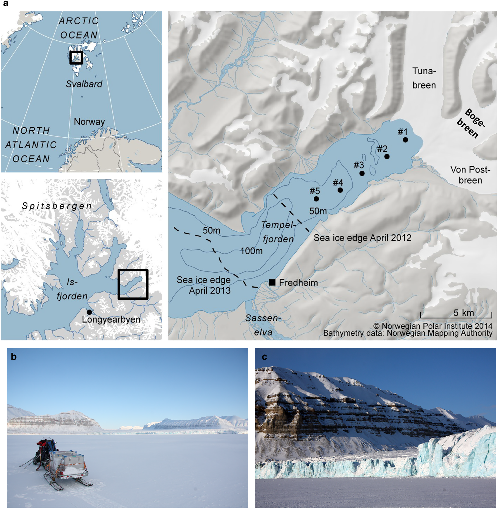
Fig. 1. (a) Map of study area in Tempelfjorden, northeast of Longyearbyen, Svalbard. Black dots indicate sampling stations (see also Table 1), dashed lines show the approximate location of the fast-ice edge in April 2012 and April 2013, (b) Tempelfjorden in April, surrounded by carbonate-rich mountains and the glaciers of Tunabreen, Bogebreen and Von Postbreen in the inner part of the fjord, (c) the glacier front of Tunabreen (station 1). Photos: Agneta Fransson.
Tempelfjorden has active seasonal sea-ice formation and is regarded as a coastal polynya, a so-called ‘sea-ice factory’. In Tempelfjorden, sea ice usually starts to form in November and breaks up between April and July (Svendsen and others, Reference Svendsen, Beszczynska-Møller, Hagen, Lefauconnier and Tverberg2002; Nilsen and others, Reference Nilsen, Cottier, Skogseth and Mattsson2008, Reference Nilsen2013). However, the timing of sea-ice formation and melt, as well as the location of the sea-ice edge, has large interannual variability in western Spitsbergen fjords (Cottier and others, Reference Cottier2007; Gerland and Renner, Reference Gerland and Renner2007; Pavlova and others, Reference Pavlova, Gerland, Hop, Hop and Wiencke2019). Information on sea-ice conditions from satellite-derived ice charts from 2012 show that the fjord was largely open until mid-January (Figs 2a and b), and had open drift ice conditions by mid-February in 2012 (Fig. 2c). By mid-March, the fjord was mainly covered by open drift ice with very closed drift ice developing in the north (Fig. 2d). In April, the fast ice had disappeared in large parts of the fjord and was again covered by very open drift ice, except in the north (Fig. 2e). The warm temperatures resulted in the late sea-ice formation in autumn and winter 2012 (Fransson and others, Reference Fransson2015a). In mid-December 2012, the fjord was still mainly open (Fig. 2f), a condition that changed drastically in February when very close drift ice was present (Fig. 2h). By mid-March 2013, fast ice covered the whole fjord and the ice edge extended more than 5 km further out in the fjord, compared to the ice edge in 2012, out to the mouth of the river Sassenelva (Fig. 1a and 2i). Sea-ice formation continued, and by mid-April 2013 the fast-ice cover extended to outside of Tempelfjorden (Fig. 2j; Figs 1b and c) The rapid transition from open drift ice to fast ice between January and March in 2013 was not observed in 2012. However, it is interesting that the ice situation between December and January was similar in both 2012 and 2013 (Figs 2a–2g).

Fig. 2. Sea-ice cover in the Isfjorden system with Tempelfjorden indicated in the black square for selected dates: (a) 15 December 2011, (b) 16 January 2012, (c) 15 February 2012, (d) 16 March 2012, (e) 16 April 2012, (f) 28 December 2012, (g) 15 January 2013, (h) 15 February 2013 (i) 15 March 2013 and (j) 15 April 2013. Data were obtained from the Ice Service of the Norwegian Meteorological Institute (MET, http://cryo.met.no/). Ice chart color scheme shows very open drift ice (1–4/10ths, green), open drift ice (4–7/10ths, yellow), close drift ice (7–9/10ths, orange), very close drift ice (9–10/10ths, red) and fast ice (10/10ths, grey).
Svalbard fjords are influenced by several freshwater sources, mainly from direct input of glacial ice or meltwater (calving or ablation), local precipitation, river runoff and sea-ice melt (Svendsen and others, Reference Svendsen, Beszczynska-Møller, Hagen, Lefauconnier and Tverberg2002). The river Sassenelva is located southwest of Fredheim (Fig. 1a). Two drainage basins surround the area (Sassenelva is not included in these two basins); the northern drainage basin where our main study took place has an area of 785 km2 and is ~58% glacier-covered (Hagen and others, Reference Hagen, Liestøl, Roland and Jørgensen1993).
Three glaciers drain into Tempelfjorden: two land-terminating glaciers (von Postbreen and Bogebreen; Figs 1b and c), and a tidewater glacier, Tunabreen, which is also a surge-type glacier (Flink and others, Reference Flink2015). Surging is a cyclical process in which a glacier alternates between quiescent periods with low velocities and frontal retreat, and short periods with high velocities, during which ice is transferred from the upper basin, and the front advances significantly into the fjord. Because glacier elevations become lower after a surge, there is an increase in glacier melt during summer, but more significantly, surging leads to greater mineral and sediment fluxes to the fjord (Sevestre and others, Reference Sevestre2018).
All three glaciers are the major sediment sources in the northern basin of our study area; here, the bedrock is dominated by carbonate and evaporitic rock (Dallmann and others, Reference Dallmann, Ohta, Elvevold and Blomeier2002). Tunabreen has surged four times since the first observations were made in the early 1900s (Hagen and others, Reference Hagen, Liestøl, Roland and Jørgensen1993), most recently in 2002–04 (Flink and others, Reference Flink2015) and now again, in 2016–18 (Sevestre and others, Reference Sevestre2018). Consequently, this means that Tempelfjorden has received varying amounts of freshwater and glacier sediment. Forwick and others (Reference Forwick2010) reported further that the waters emanating from Tunabreen and von Postbreen drainage basins consist of ~30% dolomite (CaMg(CO3)2) and 18% calcite (CaCO3), which can contribute with carbonate (CO32−) and calcium ions (Ca2+) to the fjord water and sea ice. This implies that glacial melt and drainage water from these glaciers have the potential to influence the CO2 system, ocean acidification state and the oceanic CO2 uptake (Fransson and others, Reference Fransson2015a). In the outer basin, most particles originate from the river Sassenelva (Fig. 1a), which mostly carries particles of silicate but also carbonates (Forwick and others, Reference Forwick2010).
We used air temperature and precipitation data from the meteorological station at Longyearbyen airport (Webpage: seklima.met.no/observations, Longyearbyen airport) to study the difference in climate between the 2 years. During the period 1971–2017, Svalbard experienced atmospheric warming of between 3 and 5°C, with the largest warming observed in the inner fjords (Hansen-Bauer and others, Reference Hansen-Bauer2019). The period from December 2011 to March 2012 was significantly warmer than the 50-year long-term mean air temperature from 1964 to 2014. Average air temperature for the period January–March in 2012 was −4.8°C, which was +11°C above the long-term mean (1964–2014). The corresponding values for the same period in 2013 were −11 and +4.6°C above the long-term mean. Although winter 2013 was warmer than the long-term mean, it was much cooler than in 2012. The air temperature in March 2013 was 1.4°C warmer than the long-term average. The sum of precipitation between January and March in 2012 was 97 mm (300% above the long-term mean), three times higher than the corresponding value of 31 mm in the same period in 2013.
Data and methods
Sampling
We sampled sea ice, brine, snow/brine skim, glacier ice, and the upper water column (ice/water interface, 0–2 m), from the glacier front to the outer parts of the fjord near the fast ice edge (ice edge in 2012; Figs 1a–c; Table 1). Table 1 summarizes the station locations, dates, types of sample, snow and sea-ice thickness, brine sampling depths, air temperature and a number of samples. The most extensive sampling was performed in April 2012 (five stations) and April 2013 (four stations), with limited sampling performed in January (one station), March 2012 (three stations) and September 2013 (two stations).
Table 1. Summary of the sampling dates, and locations for each station (Stn#), sampling type, and data on sea ice thickness (Th ice), snow depth, brine sampling depths and air temperature (T air). Location of the glacier front (GF) is in the inner part of the fjord (Stn #1) and the ice edge in the outer part of the fjord. Sample types are denoted ‘ice’ for sea ice, ‘uiw’ for under-ice water, ‘glac’ for glacier ice, ‘snow’ for snow (including brine skim) and ‘brine’ for brine

GF, indicates the locations of sampling of glacial ice, three samples at each location; N/a, not applicable.
Sea-ice cores were sampled using an ice corer (Kovacs®, Ø = 0.09 m). The sea ice in January was collected using a stainless-steel saw to cut chunks from the thin ice. The ice cores were divided into 10 cm sections, which were individually placed in plastic bags and put into an insulated box to avoid further ikaite precipitation due to freezing outdoor temperatures. The samples were transported to the laboratory at the University Centre in Svalbard (UNIS, Longyearbyen), and immediately transferred to gastight Tedlar® bags, to initiate the ice melting as soon as possible and avoiding long-term storage in −20°C (to avoid producing more ikaite crystals). Saturated mercuric chloride was added (100 μL for 10 cm ice, ~500 mL melted ice) to halt biological activity. The same treatment was performed on ice samples cut directly from the glacier or from ice pieces found on the beach at the glacier front. After sealing the bags, the air was removed from the bag using a vacuum pump. The bulk sea-ice samples (hereafter referred to as sea ice) were thawed in darkness and at +4°C to preserve the potential ikaite crystals within the sample; melting time was ~24–48 hour. While thawing, the sea-ice samples were regularly checked visually for the presence of different forms of solid calcium carbonate. If detected, crystals were carefully removed from the melted sea-ice sample bag using a pipette and stored in 50% ethanol at −20°C for analysis. Smaller calcium carbonate crystals will not be detected using this method, and are dissolved during the melting. This is therefore qualitative rather than a quantitative method to identify crystals present in the samples.
During the ice-coring, brine samples were collected (Table 2) into 100 ml borosilicate glass bottles from partially drilled holes in the ice, so-called sackholes. The brine, which had seeped into sackholes in the ice (Table 1) was collected with a plastic syringe with PVC tubing and transferred to bottles. During seepage, the sackholes were covered with a lid to ensure that snow was not falling into the hole and alter the measurements. The seeping time for the brine was up to 30–40 min, for sample volumes of 50–100 mL, hence some gas exchange may have taken place.
Table 2. Median, standard deviation (Std dev), minimum (min) and maximum (max) values of physical and chemical properties of temperature (T, °C), salinity (S), total alkalinity (A T, μmol kg−1), total dissolved inorganic carbon (DIC, μmol kg−1), pH in situ, partial pressure of CO2 (pCO2, μatm), carbonate ion ([CO32−], μmol kg−1), calcium carbonate saturation for calcite (ΩCa), nitrate ([NO3−], μmol kg−1), phosphate ([PO43−], μmol kg−1) and silicate ([Si(OH)4], μmol kg−1) concentrations, and isotopic oxygen ratio (δ 18O, ‰ ) in sea ice (ice), brine, snow (snow, including brine skim), glacier ice (glacier), and under-ice water (UIW)

Samples of snow at the ice surface were sampled in duplicates with a Teflon© ladle from a surface area of 1 m2 for each sample. Where the snow thickness was >5 cm (Table 1), we sampled snow at 5 cm vertical depths intervals. Occasionally, the snow samples at the ice surface contained brine, referred to as brine skim. All snow samples were placed in Ziplock® plastic bags in the field, put into an insulated box, and thereafter transferred into gastight Tedlar© bags in the laboratory. Air was gently removed from the bag using a vacuum hand pump, and the samples melted. The brine-skim and snow samples were thawed in +4°C in darkness. The melted volume was ~1 L per sample.
UIW samples were collected through the ice core holes using a 500 mL Teflon water sampler (GL Science Inc., Tokyo, Japan) in 2012. Water samples were collected directly from the water sampler into borosilicate glass bottles (250 mL) using silicon tubing for the CO2 system measurements, samples for nutrient measurements were collected in 125 mL Nalgene® bottles, and samples for δ 18O samples were collected in 25 mL Wheaton bottles, whose caps were sealed with Parafilm®. The carbonate system sample bottles were opened to add mercuric chloride and quickly re-closed.
In 2013, a 2.5 L water sampler (Limnos®) was used. Due to cold and harsh conditions in 2013, as well as challenging transportation using snow mobiles and sledges to and from the sampling sites (2 hours one way), water samples were collected and contained without headspace in unbreakable and inert HDPE Nalgene® bottles (500 mL) until processing in the lab after ~5 hours, assuming insignificant effect on the samples. In 2013, immediately after return to the laboratory, the water samples for the carbonate system were carefully transferred to 250 mL borosilicate bottles using silicon tubing to prevent contact with air and preserved with saturated mercuric chloride (60 μL to 250 mL sample, 120 μL for ice). Samples for nutrients and δ 18O were collected as in 2012.
In both years, the sampled water in the field was immediately placed in an insulated box to prevent freezing. The carbonate system and δ 18O samples were stored in +4°C and dark before analysis, and the nutrient samples were frozen and kept at −20°C.
Determination of physical properties
Sea-ice temperature was measured on site, immediately after the ice core was recovered, at 5-cm intervals using a digital probe (Testo 720) with a precision and accuracy of ±0.1°C. The holes for temperature measurement were slowly drilled with a clean stainless-steel bit, such that heating induced by drilling was negligible. The temperature of brine was measured in the sackhole before the transfer to a sample bottle, and the temperature of the UIW was measured in the sample bottle immediately after sampling, using the same handheld digital probe.
Salinity of the melted sea ice (bulk ice), brine skim, snow and UIW were measured using a WTW Cond 330i conductivity meter, with a precision and accuracy of ±0.05.
The brine-volume fraction (BV) in sea ice can be determined, based on the requirement that there is phase equilibrium between brine and ice, using the parameterizations of Cox and Weeks (Reference Cox and Weeks1983). Since more than 78% of the sea ice was colder than −2°C, BV can be described as a function of bulk-ice salinity (S) and absolute (ABS) ice temperature (T, °C) using a simplified formulation by Frankenstein and Garner, (Reference Frankenstein and Garner1967) derived from Assur, (Reference Assur1960):

This simplified BV formulation introduces an uncertainty of a maximum of 0.2% (at the coldest temperatures) in the calculations.
Concepts of percolation theory have previously been applied to sea ice (Golden and others, Reference Golden, Ackley and Lytle1998) to explain the origin of the critical porosity (percolation threshold) of sea ice, i.e. the porosity below that sea ice becomes virtually impermeable to fluid flow. Cox and Weeks (Reference Cox and Weeks1975) report that no brine drainage from sea ice was observed for total porosities below a BV of 0.05. Ice temperature fundamentally controls the ice porosity (Petrich and Eicken, Reference Petrich, Eicken, Thomas and Dieckmann2010). Golden and others (Reference Golden, Ackley and Lytle1998) investigated the sea-ice porosity and the percolation threshold of sea ice. Below a given BV threshold (below 5% for ideal, columnar ice) (Golden and others, Reference Golden, Ackley and Lytle1998, Reference Golden, Eicken, Heaton, Miner and Pringle2007), sea ice becomes impermeable to fluid flow, and above this threshold chemical substances dissolved in sea-ice brine are highly mobile (Cox and Weeks, Reference Cox and Weeks1975, Reference Cox and Weeks1983; Loose and others, Reference Loose, McGillis, Schlosser, Perovich and Takahashi2009, Reference Loose2011). Gas-bubble transport in brine channels is thought to be possible above a brine-volume threshold of ~7.5% (Zhou and others, Reference Zhou2013). The ice becomes less permeable as BV decreases, (e.g., Golden and others, Reference Golden, Ackley and Lytle1998, Reference Golden, Eicken, Heaton, Miner and Pringle2007; Loose and others, Reference Loose, McGillis, Schlosser, Perovich and Takahashi2009, Reference Loose2011), and both gas and liquid transport decreases.
For the calculation of meteoric water fractions in sea-ice cores, the isotopic composition of a sample can be used to indicate to what extent a sample is of marine or meteoric origin. Stable oxygen isotopes (δ18O) have previously been used to better understand Arctic estuarine processes (e.g. Macdonald and others, Reference Macdonald, Paton and Carmack1995; Kuzyk and others, Reference Kuzyk2008; Crabeck and others, Reference Crabeck2014). To estimate the amount of meteoric water in sea ice (FMW) we use the relation derived by Macdonald and others (Reference Macdonald, Paton and Carmack1995):

where ɛ (1.8) is the fractionation factor estimated from δ 18O values measured from upper 20 m of the surface water (UIW) in this study, which agrees with the fractionation factor estimated by Alkire and others (Reference Alkire, Nilsen, Falck, Søreide and Gabrielsen2015) in Svalbard fjords. Here we used a δ 18O value of −15.7 ‰ for glacier ice (δ 18OMW) and 0.55 ‰ for seawater (δ 18Osw) endmembers (Fransson and others, Reference Fransson2015a). The δ 18Oice values are from this study. Sea-ice formation causes fractionation (ɛ) in δ 18O, relative to the water from which it is formed. Due to fractionation upon evaporation and precipitations, snow or rain precipitating from an air mass are progressively depleted in δ 18O, with respect to the seawater source (Eicken and others, Reference Eicken2005). Using the ɛ of 2.2 from the study in a Hudson Bay estuary in the Arctic (Kuzyk and others, Reference Kuzyk2008), the FMW estimates would be 3% larger.
In 2012 and 2013, field observations and ice charts from the Ice Service of the Norwegian Meteorological Institute (MET, http://cryo.met.no/) were used to map the ice conditions. Figs 2a–j show the sea-ice coverage for the Isfjorden system and Tempelfjorden before and during part of our field periods, where the ice chart color scheme delineates very open drift ice (1–4/10ths, green), open drift ice (4–7/10ths, yellow), close drift ice (7–10/10ths, orange), very close drift ice (9–10/10ths, red) and fast ice (10/10ths, grey).
Determination of chemical properties
Melted ice (sea ice and glacier) and snow (including brine skim), brine and UIW were analysed for total alkalinity (A T), total dissolved inorganic carbon (DIC), dissolved inorganic nutrients: nitrate-nitrite ([NO3−]), phosphate ([PO42−]) and silicate ([Si(OH4)]), and stable oxygen isotopic ratio (δ 18O). DIC and A T were analyzed within 6 months after collection, either in the laboratory at University Centre in Svalbard (UNIS, Longyearbyen) or at the Institute of Marine Research, Tromsø, Norway. Analytical methods for DIC and A T determination in seawater samples are described in Dickson and others (Reference Dickson, Sabine and Christian2007). DIC was determined using gas extraction of acidified sample followed by coulometric titration and photometric detection using a Versatile Instrument for the Determination of Titration carbonate (VINDTA 3C, Marianda, Germany). The DIC instrumentation was used for all types of samples. Routine analyses of Certified Reference Materials (CRM, provided by A. G. Dickson, Scripps Institution of Oceanography, USA) ensured the accuracy and precision of the measurements. The average standard deviation from triplicate CRM analyses was within ±1 μmol kg−1 for all sample varieties.
Total alkalinity (A T) in UIW was determined from potentiometric titration with 0.1 N hydrochloric acid in a closed cell using a Versatile Instrument for the Determination of Titration Alkalinity (VINDTA, Marianda, Germany). Samples with A T are significantly different from seawater A T, such as melted ice, snow, brine skim or brine, were determined using an automated system for potentiometric titration in an open cell using 0.05 N HCl (Methrohm© Titrando system, Switzerland), described in Mattsdotter and others (Reference Mattsdotter-Bjørk, Fransson, Torstensson and Chierici2014). This method allows a smaller sample volume (40 mL) and a low HCl concentration allowed for improved determination of low A T in melted sea-ice samples, as well as analyses of samples with low volume such as brine samples. The average standard deviation for A T, determined from triplicate CRM measurements, was ±2 μmol kg−1 for both A T instrumentation systems.
We used DIC, A T, salinity, temperature, and depth for each sample as input parameters in a CO2-chemical speciation model (CO2SYS program, Pierrot and others, Reference Pierrot, Lewis and Wallace2006) to calculate all the other parameters in the CO2 system, such as CO2 concentration ([CO2]), carbonate-ion concentration ([CO32−]), bicarbonate-ion concentration ([HCO3−]) and partial pressure of CO2 (pCO2). We used the HSO4− dissociation constant of Dickson (Reference Dickson1990), and the CO2-system dissociation constants (K*1 and K*2) estimated by Mehrbach and others (Reference Mehrbach, Culberson, Hawley and Pytkowicz1973) modified by Dickson and Millero (Reference Dickson and Millero1987), since they have been shown to be valid also for sub-zero temperatures (Millero and others, Reference Millero2002; Fransson and others, Reference Fransson2015b) down to −21.4°C (Marion, Reference Marion2001). Brine concentrations of A T (A TBr) were calculated using the brine-volume fraction (BV, Eqn 4) and the bulk sea-ice concentrations of A T.
An internal consistency check performed on 100 data points of each A T, DIC and pH from measurements in Antarctic bulk sea ice showed a bias between calculated and measured DIC of ±11 μmol kg−1 (Fransson and others, Reference Fransson, Chierici, Yager and Smith2011). Similar results were showed in bulk sea ice from winter in the Kongsfjorden, where DIC deviated <±3 μmol kg−1 with a standard error of 11 μmol kg−1 using the same dissociation constants as here. Using a standard error of 11 μmol kg−1 in DIC data and ±2 μmol kg−1 for A T for sea ice and brine results in a calculated uncertainty of <±5 μatm in calculated pCO2. Delille and others (Reference Delille, Jourdain, Borges, Tison and Delille2007) found a consistency of ±25 μatm in sea-ice melt, based on comparison between direct and calculated pCO2 values. Brown and others (Reference Brown2015) estimated consistency in high salinity sea-ice brines and estimated consistency to be ~±45 (bias of 85 μatm) in the calculated pCO2 from a combination of A T and DIC for the same carbonate dissociation constants used in this study in the CO2SYS program. In summary, the uncertainty range in calculated sea-ice brine pCO2 between 5 and 85 μatm indicated that the internal pCO2 variability in sea-ice brine is larger than the uncertainty.
The ratio between A T and DIC (A T:DIC) can theoretically be used to investigate the effect of precipitation and dissolution of CaCO3 (Rysgaard and others, Reference Rysgaard, Bendtsen, Pedersen, Ramløv and Glud2009, Reference Rysgaard2012; Fransson and others, Reference Fransson2013). However, due to larger seasonal variability in DIC as a result of biological processes and air-sea CO2 exchange than in A T, the ratio between A T and salinity (A T:S) is less affected by these processes, hence is used here. The A T:S ratio has previously been used to estimate the effect of precipitation and dissolution of ikaite on A T in sea ice (e.g. Rysgaard and others, Reference Rysgaard, Bendtsen, Pedersen, Ramløv and Glud2009, Reference Rysgaard2013; Fransson and others, Reference Fransson2013). A seawater A T:S ratio of 66 is used in this study, derived from averages of A T and salinity in Fransson and others (Reference Fransson2015a). A higher A T-S ratio in sea ice than that of seawater indicates the addition of A T mainly due to dissolved CaCO3. The seawater A T:S ratio can vary both spatially and temporally, and may include effects from sea-ice derived brine, which is not accounted for. Insignificant effects due to biological processes are not considered.
By normalizing A T to a reference salinity and assuming insignificant effect on A T from biological production, the main cause for the A T change is attributed to CaCO3 dissolution or precipitation. To compare the chemical concentrations in sea ice (lower salinity) with the concentrations in seawater, the sea-ice concentrations were salinity-normalized (using dilution line) to a salinity of 34.9, obtained from Tempelfjorden seawater salinity in April 2013 (Fransson and other, Reference Fransson2015a). Based on salinity-normalized A T and DIC to a seawater reference salinity of 34.9, we calculated [CO32−]norm and [HCO3−]norm in the sea ice, using CO2SYS (Pierrot and others, Reference Pierrot, Lewis and Wallace2006).
The nutrient concentrations (nitrate + nitrite, [NO3−]) phosphate ([PO43−]) and silicate ([Si(OH)4]) were analyzed in liquid phase in all samples by colorimetric determinations on a Flow Solution IV analyzer (O.I. Analytical, USA) with routine sea-water methods adapted from Grasshoff and others (Reference Grasshoff, Kremling and Ehrhardt2009). The Analyzer was calibrated using reference seawater from Ocean Scientific International Ltd. UK, and analytical detection limits were obtained from three replicate analyses on the reference seawater. Analytical detection limits were 0.15 μmol kg−1 for nitrate + nitrite, and 0.02 μmol kg−1 for phosphate and silicate, respectively.
Stable oxygen isotopic ratios (δ 18O) were analyzed using a Picarro L2120-i Isotopic Liquid Water Analyser with High-Precision Vaporizer AO211 and Thermo Fisher Scientific Delta V Advantage mass spectrometer with Gasbench II. Different methods were used because we used different laboratories for the samples collected in 2012 and 2013. The isotope values using both methods are reported in the common delta (δ) notation relative to Vienna Standard Mean Ocean Water (VSMOW). The reproducibility of replicate analysis for the δ 18O measurements was ±0.1 ‰ for both the Picarro (2012 samples) and for the Gasbench II (2013 samples).
Section plots and interpolation were performed in Ocean Data View software version 4.7 (Schlitzer, Reference Schlitzer2015).
Qualitative analysis of crystals in particles
Mineralogical phase identification was done using a WITec alpha 300 R (WITec GmbH, Germany) confocal Raman microscope. The measurements were done using an excitation wavelength of 488 nm and an ultra-high throughput spectrometer (UHTS 300, WITec GmbH, Germany) with a grating, 600/mm, 500 nm blaze. The samples were placed in a glass Petri dish filled with crushed ice and immediately measured using a water submersible objective (20 × Olympus). Raman measurements allow a reliable identification of carbonate minerals based on their distinct molecular spectra, which are related to the inelastic scattering of light (e.g. Gillet and others, Reference Gillet, Biellmann, Reynard and McMillan1993; Nehrke and Nouet, Reference Nehrke and Nouet2011).
Results
Physical and chemical characteristics
The contrasting sea-ice conditions between the 2 years were confirmed by our field observations and measurements (Table 1). The sea-ice thickness in April 2012 was at a maximum of 54 cm at the glacier front (station 1, Figs 1a–c, Table 1), and decreased towards the ice edge, where it reached 23 cm (station 5, Table 1). In April 2013, the maximum sea-ice thickness was 84 cm at the glacier front (station 1) and 64 cm at station 5, ~5 km from the ice edge in 2013 (Table 1). The thinner sea ice in April 2012 was likely due to slower sea-ice growth due to warmer atmospheric conditions in 2012 than in 2013 (Table 1). Snow thickness was 6 cm at the glacier front (station 1) and 5 cm at the ice edge (station 5) in April 2012 (Table 1). In 2013, the snow thickness was 6 cm at the glacier front (station 1) and 4 cm at station 5 (Table 1). Freeboard was positive for all stations and years.
Vertical profiles of sea-ice temperature, salinity, stable oxygen isotopic ratio (δ 18O), brine-volume (BV) fraction and freshwater fraction along the fjord in April 2012 and April 2013 show the physical characteristics of the sea ice from the glacier front to the ice edge (Figs 3a–j). In both years, the coldest sea ice was found at the snow/ice interface (top); temperatures increased almost linearly towards the bottom ice (Figs 3a and b), which was at the seawater freezing point (~−1.9°C). In April 2012 and 2013, the top ice was ~−8°C at the glacier front. In April 2012, the top ice gradually increased towards the ice edge to reach ~−6°C. In April 2013, the top ice was generally colder (−12°C) throughout the rest of the stations. The bottom sea ice in 2012 was slightly colder at the glacier front than in 2013, likely due to the colder glacial water.

Fig. 3. Sea-ice bulk physical properties and freshwater content in April 2012 and April 2013 along the section from the glacier front (GF, 0 km on x-axis, station #1) to station #5 (8 km on the x-axis) of: (a, b) sea-ice temperature (°C), (c, d) salinity, (e, f), isotopic oxygen ratio (δ 18O, ‰ ), (g, h) brine volume in fractions (BV, fraction), where the white solid line indicates the boundary of BV <0.05, and (i, j) fresh water fractions (FMW). Dots denote the sampling depth in the ice. The dark field shows the under-ice water and the ice-water boundary. Note that station #3 was not sampled in 2013, thus the values between station #2 and #4 are extrapolated and should be interpreted with caution.
Sea-ice salinity (Figs 3c and d) was generally higher in the top and bottom ice than in the middle, a typical C-shape pattern indicating first-year ice (Malmgren, Reference Malmgren1927; Thomas and others, Reference Thomas, Papadimitriou, Michel, Thomas and Dieckmann2010). This pattern was more pronounced in April 2013 than in April 2012. The lowest sea-ice salinity measured was ~2 in April 2012 and ~5 in April 2013, both observed in the middle of the sea ice at the glacier front (Figs 3c and d). In April 2012, there was no pronounced salinity increase towards the bottom ice, which was likely due to warmer UIW in the outer part of the fjord, than in April 2013 (Table 2). Sea-ice salinity increased towards the ice edge (station 5) in both years. The highest salinity was 11 in April 2012 (in the top 10 cm of the ice at station 4) and 9 in April 2013 (at the bottom ice at station 2) (Figs 3c and d).
The δ 18O values in the sea ice were mostly positive (0–2.5 ‰ ), except for some negative values found in a few ice cores near the glacier in 2012 and at the outermost station (station 5) in 2012 (Fig. 3e). In April 2012, there was large δ 18O variability along the section, with the lowest δ 18O values of −8 ‰ near the glacier front (station 1), decreasing from top to bottom, and as high as 2.5 ‰ (near the ice edge) (Fig. 3e). At station 4, the salinity in the top 10 cm ice in 2012 was the highest and δ 18O was negative, which indicates that it was not only influenced by seawater. In 2013, a few negative δ 18O values of −2.8 ‰ were found at the bottom ice near the glacier front; otherwise δ 18O values were positive in all other ice depths with a median value of 1.8 ‰ and a maximum of 2.4 ‰ (Fig. 3f).
In April 2012, BV ranged between 2% (fraction 0.02) in top 10 cm of the sea ice at the glacier front (station 1) and 13% (0.13) at bottom ice at station 2 (Fig. 3g). In general, the sea ice was permeable (BV>5%, 0.05), except for at the upper 40 cm at the glacier front. This contrasted with April 2013, in which most of the sea ice was impermeable (BV<5%, 0.05) at all stations, indicating that the sea ice was not porous enough for gas and brine transport (Fig. 3h). In April 2013, the 5% (0.05) limit of BV was observed in the upper 50 cm of the ice at the glacier front (station 1) and in the upper 30 cm at the station near the ice edge (station 5). Consequently, it was only at the bottom part of the ice gas and brine could be transported to the underlying water (Fig. 3h).
The freshwater fraction (FMW) of 0.6 in April 2012 was largest near the glacier front (Station 1; Fig. 3i) decreasing towards the ice edge to zero (station 5), except for in the upper 10 cm of the ice at stations 4 and 5 (Fig. 3i). In April 2013, the FMW of 0.2–0.3 was only observed at the bottom ice and mid-ice (30 cm) near the glacier front. All other ice depths had the FMW of <0.1 (Fig. 3j).
Figures 4a–l show the vertical concentrations in melted sea ice (bulk) of, total alkalinity (A T, Figs 4a and b), total inorganic carbon (DIC, Figs 4c and d), carbonate ion concentrations ([CO32−], Figs 4e and f), silicate ([Si(OH)4], Figs 4g and h), and nitrate concentrations ([NO3−], Figs 4i and j) along the sections in April 2012 and 2013.

Fig. 4. Sea-ice bulk properties of the chemical variables in April 2012 and April 2013 along the section from the glacier front (GF, 0 km on x-axis, station #1) to station #5 (8 km on the x-axis): (a, b) total alkalinity (A T, μmol kg−1), (c, d) total dissolved inorganic carbon (DIC, μmol kg−1), (e, f) carbonate ion concentration ([CO32−], μmol kg−1), (g, h) silicate concentration ([Si(OH)4], μmol kg−1), and (i, j) nitrate ([NO3−], μmol kg−1). Dots denote the sampling depth in the sea ice. The dark field shows the under-ice water and the ice-water boundary. Note that station #3 was not sampled in 2013, thus the values between stations #2 and #4 are extrapolated and should be interpreted with caution.
In general, A T and DIC increased from the glacier front to the ice edge (Figs 4a–d). At the glacier front, A T and DIC were lower than close to the ice edge, in a similar pattern as δ 18O. In 2012, near the glacier front, A T and DIC were lower than the corresponding values at the same station in 2013. This coincided with higher [CO32−] near the glacier front in 2012 compared to the values in 2013 (Figs 4e and f). A T (Figs 4a and b) and DIC (Figs 4c and d) followed salinity (Figs 3c and d), with the highest values typically at the top and bottom. In 2012, the [CO32−] concentrations (Figs 4e and f) in the top ice were generally higher than in the top ice in 2013 (Fig. 4f). In 2013, on the other hand, [CO32−] was generally lower at bottom ice close to the ice edge.
Silicate concentrations (Figs 4g and h), were generally depleted (near detection limit) in the fjord ice. However, notably higher [Si(OH)4] were observed throughout the ice core at the glacier front in 2012 and at the bottom ice near the glacier front in 2013. The high [Si(OH)4] near the glacier coincided with low salinity and low δ 18O in 2012. Also in 2013, the high [Si(OH)4] in the bottom ice coincided with the lowest δ 18O, although salinity was higher than in 2012. Nitrate concentrations ([NO3−], Figs 4i and j) were low and almost depleted near the glacier front in 2012. In 2013, generally higher [NO3−] were observed in all fjord ice than were observed in 2012, with higher concentrations at the bottom ice. Phosphate concentrations ([PO43−], were depleted <0.1 μmol kg−1) in April 2012 at all sites (not shown), and in April 2013, there were higher concentrations at the bottom ice (ice/water interface, not shown).
Table 2 shows the averages of physical and chemical characteristics of sea ice, brine, snow (including brine skim, glacier ice and UIW). The brine temperatures were similar for both years with mean values of −3.6°C and −4.4°C in 2012 and 2013, respectively. The mean brine salinity was lower in 2012 (salinity of 65) than in 2013 (salinity of 80). The snow temperatures varied with air temperatures, and the snow was ~−7.1°C and warmer in April 2012 than that in April 2013 of −13.8°C (Table 2). The snow salinity was about twice as high in April 2012 than in 2013. This may be caused by a larger component of brine incorporated into the snow (brine skim layer), due to warmer ice and larger BV in April 2012. The more permeable ice in April 2012, facilitated upward brine transport relative to the conditions in April 2013 (Figs 3e and f). Brine A T and DIC were highly elevated compared to A T and DIC in bulk sea ice and in the UIW, with the highest brine A T and DIC (>5000 μmol kg−1) observed in April 2013 (Table 2). In both years, the [CO32−] and calcite saturation (ΩCa) were higher in brine than in bulk sea ice and UIW, where the brine ΩCa was clearly oversaturated (ΩCa > 4, Table 2). Brine [CO32−] varied between 17 and 1061 μmol kg−1. Brine and snow [NO3−] were relatively high, particularly in 2012, with the maximum [NO3−] of 27 and 20 μmol kg−1, respectively (Table 2). Brine pCO2 ranged between 73 and 11 934 μatm and the highest A T and DIC values coincided with relatively high salinity. Bulk sea ice was undersaturated (ΩCa<1) for both years (Table 2). Glacier ice was not significant saline, nor did it contain significant amounts of nutrients, and only small amounts of A T and DIC were found in one of the samples (Table 2).
Effects of glacial water and sea-ice processes
In glacier ice, δ 18O ranged between −10 and −15.7 ‰ , and snow (including brine skim) between −6 and −17.5 ‰ , for a salinity interval between 0 and 30 (Fig. 5a; Table 2). The δ 18O and salinity relationship indicate three mixing lines depending on the different endmembers, such as seawater and meteoric water (Fig. 5a). The sea-ice δ 18O (−2.5 to 1 ‰ ) and salinity ranges were larger in 2012 than in 2013. In 2013, the sea-ice δ 18O and salinity (from 4 to 9) were generally higher in δ 18O and similar to δ 18O in seawater (0.47–0.67 ‰ ; Table 2; Fig. 5a). Snow δ 18O and salinity indicate a clear influence of brine skim. The δ 18O in brine varied between −1.5 and −9 ‰ , in a salinity range of 30–80 (Fig. 5a; Table 2). The negative sea-ice δ 18O between −2.5 and −7.5 ‰ suggest incorporation of meteoric water, snow or brine in the sea ice in 2012 (Fig. 5a). The δ 18O in snow generally followed the mixing line between glacial ice and seawater, indicating a source of brine from the ice/snow interface (brine skim) (Fig. 5a).

Fig. 5. Salinity vs (a) δ 18O, ‰ , and (b) silicate concentration ([Si(OH)4], μmol kg−1) in sea ice, glacier ice, brine, snow (including brine skim) and seawater for 2012 and 2013 in Tempelfjorden. Dashed line in Figure 5a indicates the dilution line between glacier ice and seawater (Fransson and others, Reference Fransson2015a). Dashed line in Figure 5b denotes the relationship between silicate and salinity between glacier ice and brine.
Increased meteoric water in sea ice was observed from March to April 2012 at each station, reaching the highest integrated freshwater fraction of 54% in April 2012 at the glacier front (Fig. 6a). The fraction of meteoric water decreased towards the ice edge with the lowest values of <10% in March and April 2012 at station 3, and the lowest of <5% at the ice edge in April 2013. Figure 6b shows the vertical distribution of freshwater fractions in the ice, where FMW of 0.6 (60%) was found in bottom ice in March and April 2012 at the glacier front station (Fig. 6b). This was nearly five times higher than found at any other station in April 2012 (0.1–0.15; 10–15%), and substantially higher than at any station in April 2013 (0–0.1; 0–10%; Figs 6a and b). It is evident that there was higher freshwater fractions in the bottom sea ice at stations near the glacier front (station 1) than elsewhere, for all three sampling campaigns, (Fig. 6b).

Fig. 6. The fraction of meteoric water (FMW) in sea ice as (a) integrated freshwater content (FMW, %) in the sea ice at the five stations, from the glacier front (station #1) to station #5 (8 km on the x-axis) in Tempelfjorden in March 2012 (red), April 2012 (red dotted) and April 2013 (black), and (b) the vertical distribution of FMW (as fractions) in the sea ice for each station in March 2012 (red, closed symbols), April 2012 (red, open symbols) and April 2013 (black).
In April 2012, the highest [Si(OH)4] values were observed in the ice and seawater and show large deviation from the dilution line, suggesting excess [Si(OH)4] relative to salinity (Fig. 5b). In April 2013, the [Si(OH)4] values in both seawater and sea ice were generally lower than in April 2012, and were clustered around the dilution line (Fig. 5b).
The vertical distribution of A T:S in sea ice shows elevated A T:S values relative to seawater A T:S of 66 throughout the ice core in both years. This was particularly evident at the glacier front in 2012 (Fig. 7), where the highest A T:S ratios (>80) was found in March and April 2012, with ratios up to 141 in the mid-part of the ice (Fig. 7). The highest A T:S ratios coincided with the highest FMW near the glacier front in April 2012 (Figs 6a and b). In April 2013, the A T:S ratios were lower than that in 2012, ranging between 64 and 87 (Fig. 7).
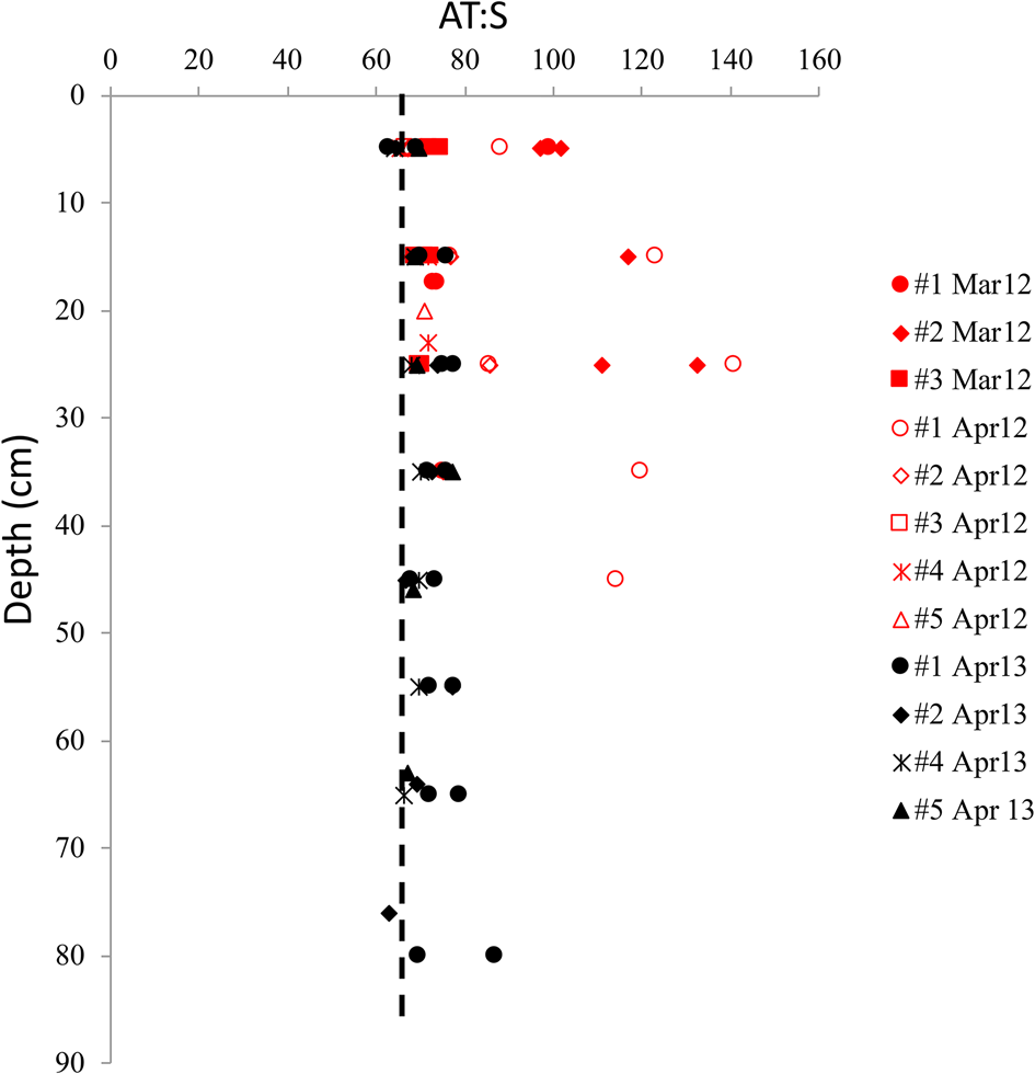
Fig. 7. The vertical distribution of the ratio between total alkalinity and salinity (A T:S) in sea ice for all sea-ice stations in March 2012 (red, filled symbols), April 2012 (red, open symbol) and April 2013 (black symbol) in Tempelfjorden. Dashed line denotes the A T:S ratio of 66 in the water column in Tempelfjorden in April 2012 and April 2013 (Fransson and others, Reference Fransson2015a).
δ 18O is a good tracer for meteoric contribution, and, when combined with the [CO32−]norm and [HCO3−]norm, gives a clue to the possible excess of [CO32−] and [HCO3−] in sea ice, relative to an average seawater salinity of 34.9. We used pure glacial ice (zero salinity) values of δ 18O of −16 ‰ assuming zero [CO32−]norm and [HCO3−]norm and average seawater δ 18O, and [CO32−]norm and [HCO3−]norm as endmembers for the dilution lines (Figs 8a and b). The seawater [CO32−]norm values were ~100–110 μmol kg−1 and [HCO3−]norm were on average 2000 μmol kg−1. The values below the respective dilution line indicates a loss of [CO32−] and [HCO3−] compared to that of seawater, and above indicates a gain (excess) of [CO32−] and [HCO3−] relative to seawater. In 2012, most of the sea ice had an excess of [CO32−] and [HCO3−], while in 2013 both excess and loss of [CO32−] and [HCO3−] were observed relative to seawater (Figs 8a and b). Consequently, the outstanding [HCO3−]norm of up to 4600 μmol kg−1 were found at the lowest sea-ice δ 18O. This implies that these elevated values are a result of dolomite dissolution.
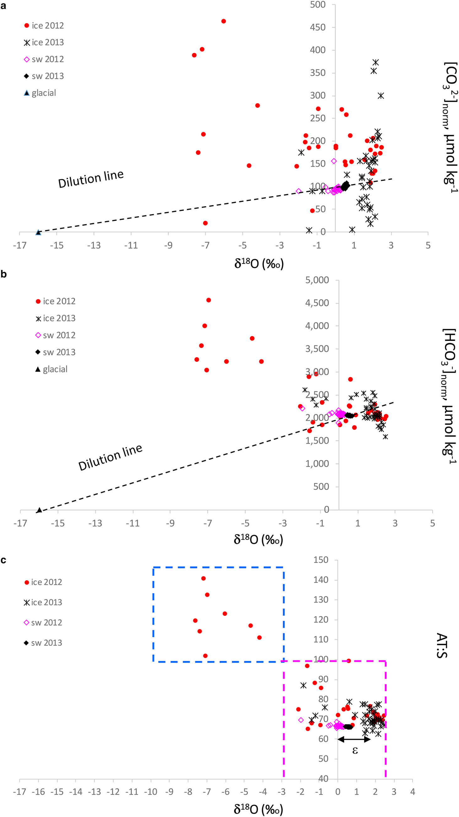
Fig. 8. Plots of δ 18O (‰) vs (a) salinity normalized [CO32−] to a seawater reference salinity of 34.9 ([CO32−]norm, μmol kg−1), (b) salinity normalized [HCO3−] to a sea-water reference salinity of 34.9 (HCO3−]norm, μmol kg−1) and (c) the ratio between total alkalinity and salinity (A T:S) in sea ice (ice), glacier ice (glacial) and seawater (sw) in 2012 and 2013. Dashed line in Figure 8a and 8b shows the dilution line between the seawater values and the glacial values assuming zero [CO32−] and [HCO3−], respectively, at zero salinity in glacier ice. Blue dashed box in Figure 8c denotes the glacial-water transported dolomite dissolution area; magenta dashed box denotes the area where ikaite and calcite dissolution is the main explanation for the A T:S values, which refer to literature A T:S values for the maximum ikaite dissolution of 84 in sea ice and 97 in frost flowers (Fransson and others, Reference Fransson2013, Reference Fransson2015b; Rysgaard and others, Reference Rysgaard2013), and the seawater value of 66 (black, Fransson and others, Reference Fransson2015a). The fractionation between sea ice and seawater, ɛ, is denoted with a black arrow in Figure 8c.
Sea ice with δ 18O values below −2.8 ‰ and A T:S ratios above 84 are assumed to be influenced by meteoric water and higher δ 18O values indicate more influence of seawater, with sea-ice A T:S ratios varying between 66 and 100 (Fig. 8c). The difference (of ~1.8 ‰ ) between the positive sea-ice δ 18O values and sea-water δ 18O is caused by δ 18O fractionation during sea-ice formation (e.g. Macdonald and others, Reference Macdonald, Paton and Carmack1995). The excess of [CO32−]norm and [HCO3−]norm at the lowest sea-ice δ 18O values in 2012 also coincided with the high A T:S ratio of up to 141, possibly indicating a contribution of carbonate ions from dissolved bedrock minerals in glacial water/meteoric water (Fig. 8c). Indeed, crystals of CaCO3 minerals were identified in sea ice, snow (including brine skim) and glacier ice (Table 3; Fig. S1). In April 2012, no minerals were found in sea ice. However, dolomite was the main mineral found in snow and glacier ice. Sea-ice samples in April 2013 contained calcite (not bedrock-transported type) while dolomite was absent in 2013. In April 2013, the snow contained mainly ikaite and calcite, particularly at station 2 and 4.
Table 3. Mineral composition of particles identified in sea ice, snow, and glacier ice in April 2012 and April 2013

Discussion
Effects of glacial water on sea-ice characteristics
In April 2012, both seawater and air temperatures were warmer than in April 2013, more precipitation fell as rain, and therefore the fresh water may have originated from several sources such as rain, snow, glacial meltwater and river runoff. Positive δ 18O indicates that sea-ice meltwater is the predominant source, negative δ 18O indicate mostly meteoric water (precipitation, glacial meltwater or river runoff). Alkire and others (Reference Alkire, Nilsen, Falck, Søreide and Gabrielsen2015) argued that it is challenging to distinguish between glacial water and river runoff. However, Killingtveit and others (Reference Killingtveit, Pettersson and Sand2003) found that the Spitsbergen freshwater sources were mainly from precipitation and glacial meltwater. The main outlet of the river Sassenelva is located at the outer part of Tempelfjorden and near Fredheim (Fig. 1a). Incorporation of freshwater flowing under the ice was found in a river-influenced shelf in the Canadian Arctic (Macdonald and others, Reference Macdonald, Paton and Carmack1995), an estuary in Hudson Bay (Kuzyk and others, Reference Kuzyk2008) and in a Greenland fjord (Crabeck and others, Reference Crabeck2014). The lowest δ 18O values in both the sea ice and seawater were found at the glacier front in 2012, not at the middle or outer stations, where a more riverine influence could be expected. The role of freshwater freeze-in in our study was indicated by the change of FMW from the glacier front to the outer station. This was particularly evident in 2012, when the mean freshwater fraction decreased abruptly from 54% at station 1 to the lowest FMW of 8% at station 3 (Fig. 6a). After station 3, FMW increased again to ~13% at the ice edge (station 5) in 2012. This slight increase could perhaps be a result of riverine influence at the outer stations. However, the FMW increase was not evident in 2013 and was generally lower (<10%) at all stations compared to that in 2012.
The δ 18O in the glacier ice ranged between −13.6 and −15.7 ‰ (Fig. 5b), which is in fair agreement with observations of δ 18O in solid precipitation from Ny-Ålesund (Svalbard), whose means is −13 ± 5 ‰ (n = 63) (D. Divine, unpublished data, 2016). One means to identify the freshwater source and to distinguish glacial meltwater from snow, rain or river inputs is to investigate the silicate concentrations. The correlation of high [Si(OH)4] and glacial water has been reported previously in Svalbard (Fransson and others, Reference Fransson2015a) and Greenland (Azetsu-Scott and Tan, Reference Azetsu-Scott and Tan1997; Azetsu-Scott and Syvitski, Reference Azetsu-Scott and Syvitski1999). In April 2012, the surface water had high [Si(OH)4] near the glacier front, suggesting the impact of glacial-water contribution, mainly by sub-glacial meltwater (Fransson and others, Reference Fransson2015a; Halbach and others, Reference Halbach2019). Indeed, the high [Si(OH)4] in sea ice were only observed at the glacier front in 2012, coinciding with the lowest δ 18O values and the highest content (68%) of frozen-in freshwater. Flink and others (Reference Flink2015) found that Tunabreen front retreat had caused the following surge events, introducing increased glacial and sub-glacial meltwater input to Tempelfjorden. Alkire and others (Reference Alkire, Nilsen, Falck, Søreide and Gabrielsen2015) found no evidence in 2013 for the incorporation of glacial meltwater in the sea ice. This supports our findings that glacial meltwater had insignificant effect in the sea ice in 2013. We conclude that most part of the fresh water incorporated in the sea ice in 2012 originated from glacial meltwater.
Calcium carbonate minerals from glacial water and sea ice
Dolomite is a common rock-forming mineral and is transported in several ways; by wind, through glacial- and sub-glacial meltwater, and through riverine transport from the drainage basin to seawater. Dolomite cannot precipitate in the sea ice as ikaite can. As seawater freezes, dolomite is incorporated in the sea ice and then transported to the surface of the ice through upward brine transport. While Alkire and others (Reference Alkire, Nilsen, Falck, Søreide and Gabrielsen2015) speculated that carbonate minerals in the glacial water could explain the elevated A T found in sea ice in 2013, they did not have any observations of minerals or measurements of DIC. Their hypothesis was confirmed in 2012, however, by Fransson and others (Reference Fransson2015a), who found glacial water derived carbonate minerals in the surface waters and in glacier ice. In this study, dolomite and calcite was found in the glacial ice and snow in 2012, but no dolomite was found in any of the sample types in 2013 (Table 3). In 2012, no ikaite was identified in any of the samples. However, the ikaite crystals could have been present in the sample at an earlier stage but were rapidly dissolved during the melting of the samples, or were too few or small to observe (Table 3). Rysgaard and others (Reference Rysgaard2013) concluded in their study that any CaCO3 crystals present in the ice cores were expected to have dissolved during sample processing and, thus, be included in the measured A T and DIC. They also found that melted bulk-ice A T in surface-ice layers (including dissolved ikaite crystals) were within the same range as analyzed ikaite concentrations, implying that most of A T originated from ikaite trapped within the surface sea-ice matrix. In 2013, ikaite was found in all sample types except sea ice and seawater. Snow (including brine skim) samples contained a large number of ikaite, which can be explained by the upward expulsion of highly CaCO3-supersaturated brine (Ω >1; Table 2). There were no ikaite observed in any bulk sea-ice samples, which could be explained by the dissolution of ikaite due to CaCO3 undersaturation (Ω <1; Table 2).
The dissolution of dolomite results in twice as large production of [HCO3−] relative to the dissolution of ikaite and calcite (Eqns 2, 4a and 4b). This fact is supported by the exceptionally high [HCO3−]norm and [CO3−]norm resulting in the large A T:S values (100–141) relative to that of seawater found in the sea ice at the glacier front in 2012 (Fig. 7; Figs 8a–c). This was also observed in the high [CO32−] and [HCO3−] above the respective dilution lines (Figs 8a and b) found in the sea ice at δ 18O values below −2.85 ‰ .
In both April 2012 and 2013, parts of the sea-ice A T:S ratios were below 100, indicating that the excess A T was mainly explained by ikaite dissolution, based on this and previous studies. However, wind-transported bedrock-originated minerals such as calcite and dolomite to seawater could be incorporated in sea ice during formation, and contributed to the A T:S ratios, when dissolved (Fig. 8b). The observations of sea-ice A T:S ranging between 66 and 85 in April 2013 and ikaite crystals identified in snow confirm that the sea ice in 2013 was influenced by A T-rich seawater, brine expulsion and ikaite dissolution in the top 30 cm of sea ice, combined with less glacial-water influence. High carbonate ion concentrations may trigger the precipitation of ikaite in sea ice. It is interesting that ikaite was not identified in any 2012 samples although the [CO32−] was relatively high in the top 10 cm in the ice in 2012, even higher than in 2013. Ikaite typically precipitates at temperatures below −2°C, thus the colder and more saline ice in 2013 with high brine concentrations of chemical solutes in sea ice and brine such as [CO32−], had a more favorable environment for ikaite precipitation than in the relatively warmer and fresher sea ice in 2012, which possibly had the presence of ikaite before the sampling in March/April. Dolomite was found in the snow in 2012, which could explain the high [CO32−] in the upper 10 cm of the ice in 2012.
Ikaite in sea ice has previously been observed and explained to result in A T:S ratios up to 84 in winter sea ice, which is clearly elevated compared to the UIW A T:S of 71 in the Canadian Arctic (Fransson and others, Reference Fransson2013). Rysgaard and others (Reference Rysgaard, Bendtsen, Pedersen, Ramløv and Glud2009) also found a AT:S ratio in wintertime sea ice of up to 84, which was explained to be caused by ikaite dissolution. In Kongsfjorden, A T:S ratios up to 73 were found in land-fast sea ice in March/April, elevated from the A T:S in surface water of 66 (Fransson and others, Reference Fransson2015b). This supports our findings from this study that ikaite dissolution in sea ice explained the excess sea ice A T:S ratios between 66 and 84 (Fig. 8c). Fransson and others (Reference Fransson2013) reported A T:S ratios between 87 and 97 in frost flowers in the Canadian Arctic in November and March (Fransson and others, Reference Fransson2013). This suggest that A T:S ratios between 84 and 100 in our study may have been a result from upward-transported brine, including ikaite crystals, which were then subsequently introduced to the top sea ice. This mechanism could explain the excess A T:S (<100) and [CO32−] in the top 10 cm in the ice in 2012 (Fig. 7; Fig. 4e). Although no ikaite crystals were identified, there may have been ikaite crystals at an earlier stage that were rapidly dissolved due to CaCO3 undersaturation and melting, or too small to discover.
Ikaite can either become trapped in the sea-ice matrix and later dissolve (gain of [CO32−]) or escape from the ice and dissolve further down in the water column (loss of [CO32−]; Fransson and others, Reference Fransson2013). Such a loss may explain the low sea ice [CO32−]norm relative to seawater values found in 2013 (Fig. 8a). Decreased [CO32−] and Ω were reported in the upper 2 m surface layer in the Canadian Arctic Archipelago in March by Fransson and others (Reference Fransson2013), which was explained to be due to ikaite precipitation within the sea ice and the downward expulsion of CO2-rich brine, increasing surface-water pCO2 and decreasing Ω. In May, increased [CO32−] and Ω were observed in the upper 2 m, mainly due to ikaite dissolution in the surface water (Fransson and others, Reference Fransson2013). In 2012, most of the sea ice indicated an excess (gain) of [CO32−], while in 2013 both excess and loss of [CO32−] were observed (Fig. 8a). The [CO32−]norm of seawater was 100 at the salinity of 34.9, meaning that the excess [CO32−] in sea ice varying between 50 and 370 μmol kg−1 was due to dissolved carbonate minerals. Rysgaard and others (Reference Rysgaard2013) found that dissolved ikaite contributed by as much as 900 μmol kg−1 to [CO32−] at the ice surface, and to ~100 μmol kg−1 at the ice bottom. Geilfus and others (Reference Geilfus2016) estimated that up to 167 μmol kg−1 of [CO32−] in sea ice was due to ikaite dissolution and Fransson and others (Reference Fransson2013) found [CO32−] values between 300 and 600 μmol kg−1 due to the dissolved ikaite.
The relatively large supply of [CO32−] and elevated A T as a result of dolomite dissolution near the glacier front in 2012 compared to in 2013 was further confirmed by the calculated A T concentration in brine (A TBV). In April 2012, the A TBV (Fig. 9a) in the top 30 cm were higher at the glacier front compared to the other stations. This was not observed in the following year, but the A TBV was clearly elevated in the top 30 cm of the ice at all other locations in the fjord in April 2013 (Fig. 9b). This supports the idea that different conditions resulted in the excess A T between the two study years. The sea ice contained five times more glacial meltwater in 2012 than in 2013, resulting in the largest excess A T at the glacier front. One explanation for the increased FMW in the upper 10 cm of the sea ice observed in 2012, between station 3 and the ice edge (station 5), together with high salinity, [CO32−], DIC, A T and negative (<0) δ 18O, could be a result of snow-ice formation including ikaite (Granskog and others, Reference Granskog2017), and not due to dissolution of dolomite transported by either meteoric water or wind. In 2013, the high A TBV at all stations except at the glacier front, was explained by progressing ice formation that caused incorporation of seawater and dissolution of ikaite.

Fig. 9. Vertical profiles of brine-volume corrected total alkalinity (A TBV, μmol kg−1) of the chemical variables in April 2012 and April 2013 along the section in the fjord, from the glacier front (GF, station #1) to station #5.
Implications for CO2 fluxes
Precipitation and dissolution of ikaite have consequences for CO2 concentrations in the brine and CO2 gas exchange. The ikaite crystals found in 2013 in the upper 30 cm of the ice indicates that precipitation had taken place in the sea ice, resulting in release of CO2 to the brine. However, the sea ice in April 2013 was not permeable (BV<0.05) in the top ice, hence no CO2 exchange with the atmosphere occurred. The brine pCO2 (Table 2) was higher (above 700 μatm) than atmospheric pCO2 (~400 μatm) in both years. The highest pCO2 of 11 000 μatm observed in the brine could be explained by local effects, such as bacterial respiration producing CO2. The presence of locally distributed bacteria was suggested by Fransson and others (Reference Fransson2015b) to be partly responsible for the elevated brine pCO2, ranging between 2983 and 18 139 μatm (median of 10 561 μatm) in a wintertime sea-ice study in Kongsfjorden in Svalbard. Miller and others (Reference Miller2011) reported high brine pCO2 > 20 000 μatm, using silicone chamber sampler (‘peepers’) to absorb CO2 from the brine and measure pCO2, in the Canadian Arctic winter, where low sea-ice temperatures below −15°C resulted in low BV and high concentrations in the brine. In our study, the sea ice was warmer, and BV was larger in April 2012, than in the study by Miller and others (Reference Miller2011), hence higher brine pCO2 could have been expected. The reason for the lower pCO2 than expected, was likely due to brine-CO2 transport through expulsion to the bottom ice (BV >0.05), where CO2 could escape to the underlying water, so-called brine pump, or escape to the top ice and atmosphere, particularly in April 2012.
Due to relatively cold temperatures and low BV, the sea ice in April 2013 was mostly impermeable (BV<5%) for gas transfer, limiting exchange with the atmosphere, such that no CO2 exchange may have occurred at this time. However, the CO2 exchange could have occurred during new ice formation, earlier than our observations. The maximum pCO2 of 1600 μatm in sea ice in April 2013 indicated a limited exchange with the surrounding, whereas in April 2012, the maximum sea-ice pCO2 was similar to that in UIW (Table 2). The top 10 cm ice in 2012 had high carbonate ion concentrations and BV >5% (permeable), allowing gas exchange, except for at the glacier front. The maximum pCO2 in snow was 5344 μatm (Table 2), suggesting brine-CO2 upward expulsion and/or ikaite precipitation mixed with snow at the ice surface, and CO2 exchange with the atmosphere. In the future climate warming scenario, the ice will become warmer, thinner and more porous and allow for increased gas permeability. However, with increased freshwater incorporated in the sea ice, the permeability may decrease. In April 2013, the bottom sea ice showed signs of ongoing primary production, which was not significant in the thinner sea ice of 2012 (Fransson and Chierici, unpublished data). The high [NO3−] values observed at the bottom ice can be either explained by brine rejection or by seawater intrusions at the ice/water interface. High [NO3−] was observed mostly in the thicker and more seawater influenced sea ice in April 2013, compared to the thinner ice of April 2012, which could explain the primary production in the bottom ice. The warmer ice (BV>5%) will have increased potential for CO2 exchange with atmosphere and water (increased mobility in warm ice). Bacterial respiration and the turnover rate of the microbial carbon loop in sea ice may increase at higher temperatures (e.g. Torstensson and others, Reference Torstensson, Hedblom, Mattsdotter Björk, Chierici and Wulff2015), hence outgassing or the transport of CO2 to the surface water may continue. On the other hand, a fresher source water resulted in less formation of dense CO2-rich brine derived from ikaite formation and decreased transport of CO2 to underlying water through the brine pump.
Scenarios of warming and increased glacial meltwater
Projections of climate change towards the end of the century show a large increase of annual runoff, caused mainly by increased glacial melting in response to strong warming, and to increased precipitation associated with the warming (Hansen-Bauer and others, Reference Hansen-Bauer2019). The Svalbard archipelago is covered by ~60% glaciers, all of which are retreating over decadal timescales, and all of which are losing mass (e.g. Kohler and others, Reference Kohler2007; Moholdt and others, Reference Moholdt, Hagen, Eiken and Schuler2010; Nuth and others, Reference Nuth, Moholdt, Kohler and Hagen2010). This mass loss is mainly caused by increased melting through warming (e.g. Kohler and others, Reference Kohler2007), thus increasing the freshwater and sediment supply to the nearby fjords and ocean. In future, warming of the air and ocean increases the melting of glaciers, ice caps and sea ice and increase river runoff in the Arctic. Consequently, this results in increased freshwater content in the surface water and sea ice, affecting the sea-ice physical and chemical characteristic and biogeochemical processes. This will have further consequences for brine rejection from sea ice, carbon transport and ocean circulation, biological processes, air-sea CO2 exchange and ocean acidification.
In our study, the colder winter 2013 led to more sea-ice formation and more brine formation, which in turn resulted in haline convection. This convection explained the elevated salinity above 35 observed under the sea ice in the top 5 m in April 2013 (Fransson and others, Reference Fransson2015a). Haline convection likely decreases because of increased freshwater runoff, similar to the situation in Tempelfjorden in winter 2012 (Fransson and others, Reference Fransson2015a). Ultimately this results in less wintertime mixing of water and stronger surface stratification when sea ice melts and additional meltwater is added from the glaciers. This may also cause less nutrient addition from subsurface waters, hence less primary production. Another consequence of increased freshwater runoff is the increased silt and sediment load to the fjord, which restricts light and limits primary production, as has been found near the glacier fronts in Kongsfjorden (Halbach and others, Reference Halbach2019). Increased freshwater fluxes enhances ocean acidification and decrease CaCO3 saturation states, as observed on the freshwater-influenced shelves in the Canadian Arctic (Chierici and Fransson, Reference Chierici and Fransson2009) as well as in Kongsfjorden (Fransson and others, Reference Fransson2016). Decreased biological CO2 consumption and possibly less contribution from buffering ions from ikaite dissolution will have a positive feedback on ocean acidification.
Conclusion
The two contrasting winters clearly showed that the amount of freshwater content in the fjord influenced the chemical and physical characteristics of sea ice. It was obvious that the lowest alkalinity, δ 18O and nitrate, and the highest silicate concentrations at the glacier front coincided with the highest freshwater fractions. Glacial and sub-glacial meltwater contributed to alkalinity in April 2012 due to the incorporation of carbonate minerals (mainly from dissolved calcite and dolomite) originating from the bedrock-influenced glacial freshwater runoff. The result of dissolved ikaite due to sea-ice processes was the main cause of the elevated alkalinity relative to salinity in the sea ice in April 2013. Since ikaite has a seawater source, precipitates in sea ice, and dissolves in the melted sea ice, brine or in underlying water, CO2 is either produced or consumed, depending on the season. This means that the magnitude as well as the net effect of CO2 exchange with the surrounding environment is difficult to predict. Regarding the bedrock-derived carbonate minerals added from an external source and not produced in sea ice, the net effect will be decreased CO2 since these minerals contribute to the seawater buffering capacity against CO2, when dissolved. This study demonstrated that the different sources and species of CaCO3 minerals play an important role in determining the final impact in the water-column chemistry. Moreover, dolomite dissolution produces twice as many bicarbonate ions as ikaite (and calcite), and hence contributes twice as much to alkalinity and buffering capacity in the water column compared to ikaite and calcite dissolution. As a result of the contrasting winters in Svalbard, glacial-water influenced fjords are affected by carbonate-rich bedrock. Accordingly, these fjords can be considered as climate laboratories and be used to project climate-change effects in other freshwater-influenced areas, such as Greenland fjords and shelves, and the shallow shelves of the Canadian Arctic Archipelago. In the context of retreating glaciers, ice caps and increased meltwater in the Arctic Ocean and fjords, the result from this study suggests that in a warmer climate, with increased glacial melt, sea ice would be formed in the fresher water, potentially with less ikaite in the sea ice and a larger influence of bedrock minerals on sea ice and water. Regardless of the specie of carbonate mineral, the contribution to the water column increases ocean CO2 uptake due to increased buffer capacity.
Supplementary material
The supplementary material for this article can be found at https://doi.org/10.1017/aog.2020.52.
Acknowledgement
This is a project within the Fram Centre flagship research program ‘Ocean acidification and ecosystem effects in Northern waters’ at the FRAM—High North Research Centre for Climate and the Environment, for financial support (A.F., M.C., M.G.). We acknowledge the Japan Society for Promotion of Science support (23–207, 24–4175, and 17H04715) for D.N. and Svalbard Science Foundation Field Grant support to M.C. (grant 1795) and D.N. (grant 1881), and T.M. (EU Regional Development Foundation, project 3.2.0801.12–0044). G.N. is supported by the DFG by grant NE 1564/1–1 (SPP1158). We also thank the three anonymous reviewers for constructive comments, improving the manuscript. Thanks also to Jack Kohler for the English proof reading. Data will be publicly available on the Norwegian Polar Institute Data Centre and Norwegian Marine Data Centre, metadata will also be available at RiS portal at www.researchinsvalbard.no, within 1 year after publication, until then contact the corresponding author. We thank the Norwegian Polar Institute (NPI) logistics and safety training in Longyearbyen, particularly thanks to Jørn Dybdahl for logistics, technical support and guiding and support in the field, the University Centre in Svalbard (UNIS) for lab facilities, and Helene Hodal Lødemel, Mikael Hedström for assistance in the field.


 Open access