


1. Introduction
The dramatic decline of Arctic-wide sea-ice extent has been one of the most visible early consequences of anthropogenic global warming (Onarheim and others, Reference Onarheim, Eldevik, Smedsrud and Stroeve2018; Stroeve and Notz, Reference Stroeve and Notz2018; Serreze and Meier, Reference Serreze and Meier2019). Along with a decline in extent, the Arctic sea ice that remains is more likely to be thin, first-year ice rather than thick, multi-year ice (Kwok, Reference Kwok2018; Mallett and others, Reference Mallett2021). Areas that were once perennially ice-covered are now seasonally ice-free (Wang and others, Reference Wang, Liu, Key and Dworak2022), and areas that were already seasonally ice-covered now have longer ice-free seasons in summer (Stroeve and others, Reference Stroeve, Crawford and Stammerjohn2016; Bliss and others, Reference Bliss, Steele, Peng, Meier and Dickinson2019). These trends are projected to continue with additional Arctic warming (Lebrun and others, Reference Lebrun, Vancoppenolle, Madec and Massonnet2019; Notz and Community, Reference Notz and Community2020; Årthun and others, Reference Årthun, Onarheim, Dörr and Eldevik2021).
The timing of summer retreat and fall advance of Arctic sea ice (‘sea-ice phenology’) has important implications for ocean wave action and coastal erosion (Overeem and others, Reference Overeem2011), marine ecosystems (Ferguson and others, Reference Ferguson2017; Lewis and others, Reference Lewis, van Dijken and Arrigo2020; Siddon and others, Reference Siddon, Zador and Hunt2020; Pagano and Williams, Reference Pagano and Williams2021), and various human activities, from marine shipping (Andrews and others, Reference Andrews, Babb and Barber2018; Li and others, Reference Li2021; Mudryk and others, Reference Mudryk2021) to hunting and fishing (Huntington and others, Reference Huntington, Quakenbush and Nelson2016; Galappaththi and others, Reference Galappaththi, Ford, Bennett and Berkes2019). For many of these stakeholders, changes in sea-ice phenology are most valuable when examined at a local or regional scale rather than Arctic-wide.
Addressing this need, Crawford and others (Reference Crawford, Stroeve, Smith and Jahn2021) analyzed the sea-ice phenology of 16 regional Arctic (and sub-Arctic) seas in 21 climate models participating in the latest iteration of the Coupled Model Intercomparison Project (CMIP6) under three possible shared socioeconomic pathways. Their goal of making future projections was limited by the presence of significant biases in historical sea-ice phenology in some regions, especially in the Hudson Bay Complex (HBC). Compared to the passive microwave record, each of the 21 CMIP6 models overestimated the length of the ice-free season in the HBC. To obtain more confident projections of future Hudson Bay sea ice, the sources of this bias need to be uncovered and addressed.
The main goal of this study is to elucidate why the majority of CMIP6 models overestimate the length of the ice-free period in the HBC during the historical period by examining the relationship between sea-ice phenology and its influencing factors. To accurately represent HBC sea-ice phenology, a model must reproduce both the average conditions for the region, and also the spatial patterns of opening, retreat, advance and closing. We examine the possibility that the ice-season model bias could be caused by unrealistically simulated surface air and ocean temperature, 10 m winds, snowfall/depth and surface albedo or coarse spatial resolution. Section 2 provides a literature review of sea-ice phenology in Hudson Bay. This is followed by a description of data and methods (Section 3), the results of the model comparisons (Section 4), a discussion of implications and limitations (Section 5) and conclusions (Section 6).
2. Background
Sea-ice phenology involves varied terminology depending on the study; compare, for example, Stammerjohn and others (Reference Stammerjohn, Massom, Rind and Martinson2012), Smith and Jahn (Reference Smith and Jahn2019), Bliss and others (Reference Bliss, Steele, Peng, Meier and Dickinson2019) and Walsh and others (Reference Walsh, Eicken, Redilla and Johnson2022). In this study, the phrase ‘ice-free period’ refers to the continuous period each year for which sea-ice concentration (SIC) is below 15%, with the beginning and ending of that period referred to as the ‘retreat day’ and ‘advance day’, respectively (Fig. 1a). The ‘open-water period’ is more broadly the continuous period for which SIC is below 80%, with the beginning and ending of that period referred to as the ‘opening day’ and ‘closing day’, respectively. The period between opening and retreat days is the ‘melt period’, and the period between the advance and closing days is the ‘growth period’. The period between closing in winter and the subsequent opening is the ‘ice-covered period’. Finally, it is often useful to consider spatial averages for the entire HBC (including Foxe Basin, Hudson Strait and James Bay), but also the differences between specific sub-regions (Fig. 1b).
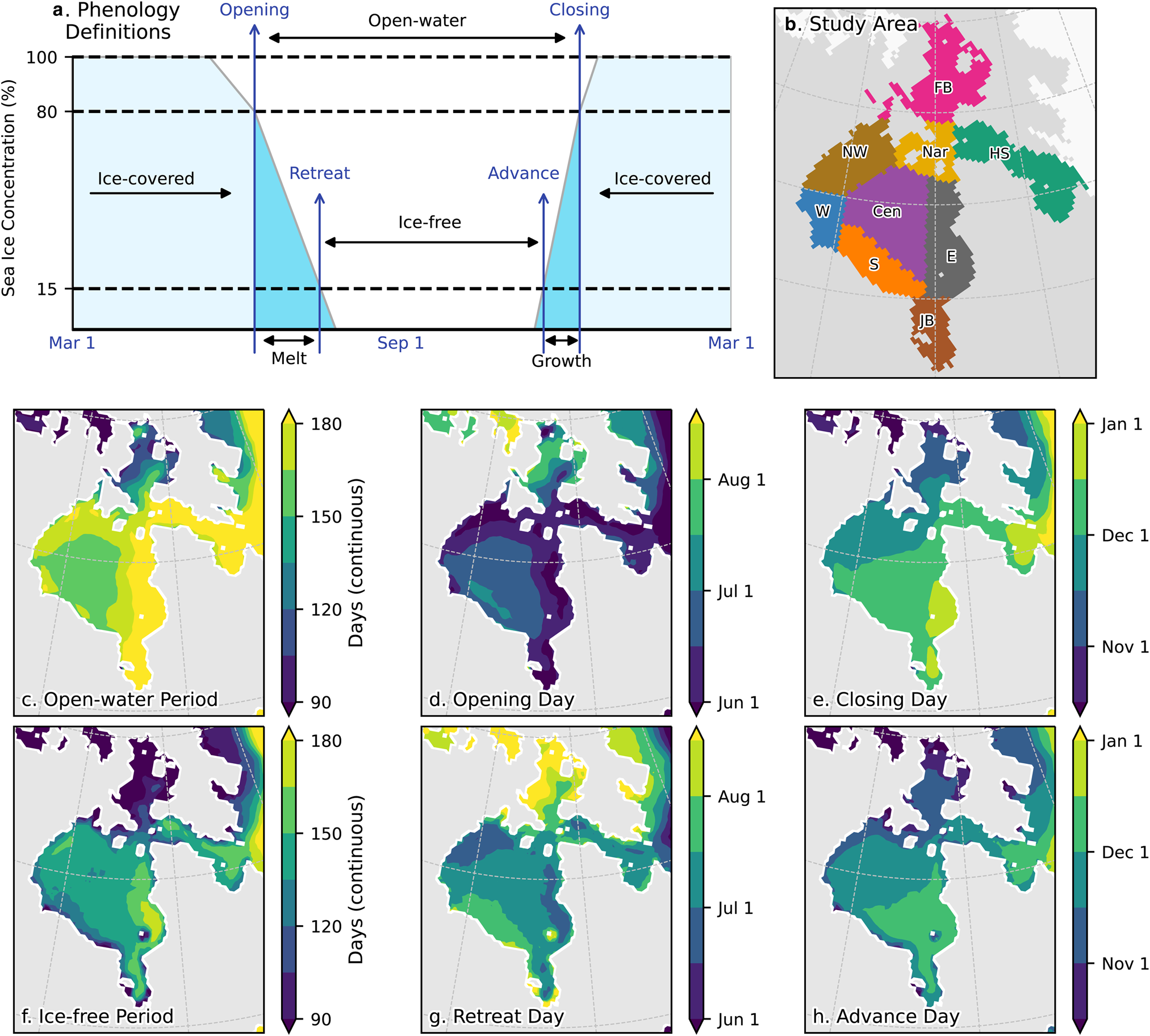
Figure 1. Climatological sea-ice phenology in the HBC (1979–2014) from observations. Definitions for sea-ice phenology periods and timing (c–h) are portrayed in a simplified schematic (a) of a time series of SIC in the HBC for a typical year. (b) Definitions for HBC sub-regions used during spatial averaging: FB, Foxe Basin; HS, Hudson Strait; Nar, the Narrows; JB James Bay; Cen, Central Hudson Bay, and NW, S, W and E refer to cardinal directions.
The ice-free period lasts 128 d on average for HBC locations, but that ranges from below 90 d in northern Foxe Basin to over 165 d in eastern Hudson Bay (Fig. 1f). Advance occurs north to south and (more subtly) west to east (Gagnon and Gough, Reference Gagnon and Gough2005; Hochheim and Barber, Reference Hochheim and Barber2010), from late October in the northern end of Foxe Basin to early December in eastern Hudson Bay and parts of James Bay (Fig. 1h). The north-to-south gradient can be attributed to the gradient in solar radiation, and therefore temperature (Hochheim and Barber, Reference Hochheim and Barber2010). Wind direction also plays a role, as offshore winds from the northwest promote cooler temperatures on the west side of Hudson Bay (Maxwell, Reference Maxwell and Martini1986; Etkin, Reference Etkin1991; Hochheim and Barber, Reference Hochheim and Barber2014). The growth period (between advance day and closing day) is <2 weeks in most places (Figs 1e, h). Model experiments have also shown some sensitivity to perturbations in river discharge, with increased fresh water in winter encouraging faster ice growth (Saucier and Dionne, Reference Saucier and Dionne1998; Lukovich and others, Reference Lukovich2021a).
Past literature describes a more complex spatial pattern of sea-ice retreat (Etkin, Reference Etkin1991; Gagnon and Gough, Reference Gagnon and Gough2005; Hochheim and others, Reference Hochheim, Lukovich and Barber2011). Opening in the HBC begins at the end of May in northwestern Hudson Bay, eastern Hudson Bay and Hudson Strait, with final retreat in these regions occurring by the end of June (Figs 1d, g). Central Hudson Bay experiences opening in late June and final retreat in early July. Despite its lower latitude, southern Hudson Bay experiences retreat in late July. Foxe Basin has the latest sea-ice retreat, with some notable sea ice left on 1 August.
As with sea-ice advance day, surface air temperature and wind direction are important influences on year-to-year variability of sea-ice retreat day. Spring atmospheric temperatures are a good predictor of spring sea-ice conditions, as sea-ice melt in the HBC is driven primarily from above (Etkin, Reference Etkin1991; Hochheim and others, Reference Hochheim, Lukovich and Barber2011; Joly and others, Reference Joly, Senneville, Caya and Saucier2011). Prior fall/winter temperatures are also decent predictors of spring sea-ice cover in Hudson Bay since a colder fall/winter tends to produce earlier advance, which in turn leads to thicker ice (Hochheim and others, Reference Hochheim, Lukovich and Barber2011; Tivy and others, Reference Tivy, Howell, Alt, Yackel and Carrieres2011). However, Gough and others (Reference Gough, Gagnon and Lau2004) showed that for many long-term Canadian Ice Service records along the HBC coast, snow depth was a stronger predictor of interannual variability in spring sea-ice thickness than air temperature. (Thicker snow cover reduces thermodynamic sea-ice growth.) Average sea-ice thickness at the end of winter varies from under 1.0 m in James Bay to ~2.5 m in Foxe Basin (Gagnon and Gough, Reference Gagnon and Gough2006). Melting from below is less important in the HBC than other Arctic regions because of the highly stable water column (Jones and Anderson, Reference Jones and Anderson1994; Saucier and others, Reference Saucier2004; Ridenour and others, Reference Ridenour2021). However, the higher volume of relatively warm river discharge in summer (St-Laurent and others, Reference St-Laurent, Straneo, Dumais and Barber2011; Yang and others, Reference Yang, Shrestha, Lung, Tank and Park2021) may help explain the relatively early sea-ice retreat in eastern Hudson Bay (Whitefield and others, Reference Whitefield, Winsor, McClelland and Menemenlis2015; Park and others, Reference Park2020).
Sea-ice dynamics are also critical to the spatial pattern of ice retreat in the HBC. Cyclonic (counter-clockwise) circulation dominates in Hudson Bay over fall and winter, largely driven by atmospheric vorticity (Prinsenberg, Reference Prinsenberg1986; Dmitrenko and others, Reference Dmitrenko2020). Wind-driven counter-clockwise circulation causes sea-ice divergence in the northwest of Hudson Bay; polynya formation is common (Bruneau and others, Reference Bruneau2021), and sea-ice retreat occurs relatively early (Etkin, Reference Etkin1991; Saucier and others, Reference Saucier2004). Sea-ice convergence occurs primarily in southern Hudson Bay and/or eastern Hudson Bay, depending on the strength of westerly winds (Saucier and others, Reference Saucier2004; Kirillov and others, Reference Kirillov2020). Convergence throughout the ice-covered season and into the melt season causes southern Hudson Bay to maintain some sea-ice cover about a month later than in the northwest (Fig. 1g; Etkin, Reference Etkin1991).
In summary, the timing of fall advance and summer retreat of sea ice in the HBC is strongly related to atmospheric temperature. The timing of summer retreat is further complicated by the importance of sea-ice thickness at the end of the growth season, which in turn depends on thermodynamic growth and sea-ice dynamics. Snow depth and river discharge also play a role in sea-ice growth and melt. Biases in any of these factors, along with model characteristics like spatial resolution or sea-ice albedo, may all contribute to any bias exhibited in sea-ice phenology.
3. Data and methods
3.1. CMIP6 data
Daily SIC from 1979 to 2014 (historical experiment) was acquired from the Earth System Grid Federation for 37 models participating in CMIP6 (Supplementary Table S1; Eyring and others, Reference Eyring2016). The first ensemble member (i.e. replicate ‘r1’) for each model was used to generate a multi-model ensemble. All data processing is conducted on the native grid, but for maps of model bias, all fields were re-projected to Polar Stereographic North (EPSG = 3413) at 25 km spatial resolution. Data from at least 27 of 37 models were available for each of the other variables of interest (Table 1). Additionally, a 23-replicate single-model ensemble was collected for all variables of interest from each of three models (EC-Earth3, IPSL-CM6A-LR and MPI-ESM1-2-LR). (Twenty-three replicates is the minimum number of replicates for these three models, and no other model had more than ten.) These three ensembles were used to estimate internal variability (see Section 3.4).
Table 1. CMIP6 variables used in this study and the sources for reference data

3.2. Observational data sources
We examine several ancillary data sources to compare observational (or quasi-observational) references against CMIP6 data. SIC is acquired from three sources. Our main source is the average of four SIC datasets derived from passive microwave satellites: the Ocean and Sea Ice Satellite Application Facility (OSISAF) product (Lavergne and others, Reference Lavergne2019), the bootstrap algorithm (Comiso, Reference Comiso2017), the NASA Team algorithm (Markus and Cavalieri, Reference Markus and Cavalieri2000) and a maximum SIC found in the latter two (Meier and others, Reference Meier, Fetterer, Windnagel and Stewart2021). Hereafter called the ‘passive microwave record’, this is our best possible observational reference, but it is not ideal for every analysis. For comparing sea-ice conditions to atmospheric variables in the European Centre for Medium-Range Weather Forecasts (ECMWF)'s Retrospective Analysis (ERA5; Hersbach and others, Reference Hersbach2020), we use SIC fields from ERA5 as our second source. ERA5 SIC is based on OSISAF but not identical. Our third source is the Pan-Arctic Ice Ocean Modeling and Assimilation System (PIOMAS), a sea-ice reanalysis (Schweiger and others, Reference Schweiger2011). We use PIOMAS to examine sea-ice volume and drift rather than observational sources to maintain mass conservation when calculating sea-ice volume budgets. All SIC products are shown in the below figures, but the passive microwave record is considered the primary reference.
Monthly surface air temperature is also acquired from multiple sources when comparing observations to models: (1) the instrument-based Berkeley Earth Surface Temperatures (BEST) dataset (Rohde and others, Reference Rohde, Muller, Jacobsen, Perlmutter and Mosher2013) is paired with the passive microwave record, (2) 2 m temperature fields from ERA5 (Hersbach and others Reference Hersbach2018, Reference Hersbach2020) are paired with ERA5 sea ice and (3) 2 m temperature fields from the NCEP-NCAR reanalysis (Kalnay and others, Reference Kalnay1996) are paired with PIOMAS since the NCEP-NCAR reanalysis provides atmospheric boundary forcings for PIOMAS (Schweiger and others, Reference Schweiger2011). Monthly fields of 10 m zonal and meridional winds are taken from ERA5 and NCEP-NCAR reanalysis as well.
A few reference datasets appear only in the Supplementary material. We use HadISST for sea-surface temperature (Rayner and others, Reference Rayner2003). Surface albedo is calculated as the ratio of upwelling to downwelling shortwave radiation from daily ERA5 fields. A comparison of six atmospheric reanalyses (Graham and others, Reference Graham2019a) found that ERA5 was most consistent with in situ observations of downwelling and net shortwave radiation over spring and summer sea ice. To estimate snow depth on sea ice, we use the combined record of AMSRE (June 2002–June 2011) and AMSRU (July 2012–December 2014) (Meier and others, Reference Meier, Markus and Comiso2018), which includes 5 d averages of snow depth on first-year ice, which covers all HBC for this period.
Most ancillary datasets are available for the entire period 1979–2014, but the passive microwave data include both spatial and temporal data gaps. A temporal gap exists for 3 December 1987 through 12 January 1988, which overlaps with the sea-ice growth season for part of the HBC. Linear interpolation using the 5 d on either side of that gap is conducted before calculation of sea-ice phenology. AMSR snow on sea-ice data are only available 2002–14. Spatial resolution ranges from 12.5 km for AMSR data, 25 km for the passive microwave SIC and PIOMAS, 0.25° for ERA5, 1° for BEST and HadISST and 1.875° for NCEP/NCAR reanalysis.
3.3. Sea-ice phenology and volume budget
For a full description of the method used to define sea-ice phenology each year, readers are referred to Crawford and others (Reference Crawford, Stroeve, Smith and Jahn2021). Briefly, daily SIC fields are first smoothed using a 5 d moving average filter to remove high frequency fluctuations. Next, the timing of each sea-ice period is defined, following the definitions in Figure 1a. The period of study is 1979–2014, which comprises the overlap between the historical CMIP6 experiment and the passive microwave satellite record. Since all gridcells in the HBC had seasonal ice during this time, it is possible to calculate regional values of every sea-ice parameter as simple area-weighted averages for the entire HBC or separate sub-regions.
A sea-ice volume budget is constructed for both CMIP6 and PIOMAS by calculating the daily change in sea-ice effective thickness [i.e. thickness (h) multiplied by concentration (C)], sea-ice advection and sea-ice divergence:

Advection (Adv) and divergence (Div) are calculated using MetPy (May and others, Reference May2022). The difference between the overall thickness change and combined growth from advection or convergence (−Div) is taken as thermodynamic growth (T), following past studies (Schroeter and others, Reference Schroeter, Hobbs, Bindoff, Massom and Matear2018; Lukovich and others, Reference Lukovich2021b).
3.4. Statistical methods
Many of the following figures include a scatter plot for which each point represents the average state (1979–2014) of two variables (x and y) in one model simulation or the reference datasets. Two other elements are included in each plot: (1) a dashed black box surrounding the reference point and (2) a dashed black regression line for the model points.
The black boxes quantify internal variability, or variability in the model output related to natural, quasi-random variations in the climate system. Internal variability of a variable is estimated as 2σ max, where σ max is the highest std dev. for that variable from the three 23-member single-model ensembles. This interval is then plotted as error bars extending from the reference dataset. Model results falling within those error bars are considered reasonable representations of observed values; in such cases, variation in internal variability is a plausible explanation for any difference. If a model falls outside the black box, this indicates bias in the x variable and/or the y variable.
Ordinary least-squares regression is used to measure the relationship between sea-ice phenology variables and other factors among the 37 models. In a few cases, extreme outliers had excessive leverage on results, so regression was re-run with those outliers removed. These cases are noted in the text. If a significant relationship exists between variables x and y, this indicates that if we knew the model bias in variable x, we could use that to predict the model bias in variable y. This would be consistent with the hypothesis that bias in variable y is caused by bias in variable x (although not prescriptive of causation). Additionally, if a significant relationship exists, we can use the average value of variable x in each model and the regression coefficient to adjust variable y from each model. The average bias in variable y will be reduced with such an exercise, so this is a form of bias correction.
4. Results
4.1. Excessive ice-free conditions in CMIP6 models
As reported by Crawford and others (Reference Crawford, Stroeve, Smith and Jahn2021), most CMIP6 models simulate unrealistically long ice-free periods in the HBC (Fig. 2b; see also maps in Supplementary Fig. S1). These biases are often large, with the multi-model mean overestimating the ice-free period by 30 d, and one model overestimating by 87 d. Out of 37 models, 27 (comprising 73% of the models) overestimate the ice-free period, one underestimates the ice-free period, and only nine are unbiased. For every sub-region, a majority of models overestimate the length of the ice-free period. Further, the multi-model mean lies beyond the range of internal variability when compared to the passive microwave record for all regions except for Hudson Strait. Bias is especially strong in southern Hudson Bay, for which only one model simulation falls within the range of internal variability (126 ± 14 d), and 31 of 37 (84%) overestimate the ice-free period by at least 28 d.

Figure 2. Comparison of sea-ice phenology in CMIP6 models and observations (1979–2014) for HBC and its sub-regions (Fig. 1b) using (a, c, e) 80% or (b, d, f) 15% SIC as the concentration threshold (as defined in Fig. 1a). The CMIP6 multi-model mean (red dot) is derived from the first member (or ‘replicate’) of each CMIP6 model historical ensemble (red bars). ERA5 (light gray) and PIOMAS (dark gray) are shown for comparison. The maximum internal variability (2σ max) from three CMIP6 single-model ensembles is used for the error bars around the mean for the passive microwave record (white dot).
On average, the bias in the ice-free period arises both because sea-ice retreat occurs 19 d too early and sea-ice advance occurs 9 d too late (Figs 2d, f). The greater bias for retreat day is driven mostly by Hudson Strait (retreat bias = −17 d and advance day bias = +4 d) and Foxe Basin (−33 and +12 d, respectively). In other sub-regions, the bias is more equally distributed between retreat and advance, with bias in retreat day being larger by a few days. Eastern Hudson Bay is the only sub-region for which more than one model simulates the retreat day as unrealistically too late, and average retreat day bias is lowest in this region at 8 d too early.
If considering the open-water period (SIC <80%) instead of the ice-free period (SIC <15%), the bias in the CMIP6 multi-model mean is greatly reduced – even eliminated in the northern sub-regions. Most notable is how the opening day (SIC falls below 80%) is timed more accurately than the retreat day (SIC falls below 15%). Therefore, whatever the source of bias, it does not cause the melt season to initiate too soon, but rather to progress too quickly (Supplementary Fig. S2). Similarly, the growth season appears to be too short, starting too late but ending closer to a time that matches observations.
Overall, then, any description of bias source(s) for HBC sea ice must explain four general observations:
(1) The ice-free season is unrealistically long across nearly all sub-regions of the HBC.
(2) The retreat day is consistently too early and the advance day is consistently too late, but the bias in retreat day is greater overall.
(3) The transition seasons (melt season in summer, growth season in fall) occur too quickly.
(4) The magnitude of bias exhibits substantial regional variability.
The following results highlight mechanisms that, if accurately simulated, would reduce the overall model bias in sea-ice phenology. Only mechanisms that proved useful for explaining HBC sea-ice bias are described. Some other mechanisms, which did not prove useful, are mentioned in Section 5.
4.2. Temperature is closely related to sea ice
Average near-surface air temperature over the HBC (hereafter ‘air temperature’) in a model is closely related to its sea-ice phenology (Fig. 3). Many models show a bias in both sea-ice phenology and air temperature, including in the season that precedes a given sea-ice event. Additionally, models that are warmer tend to have earlier retreat and later advance, which leads to a longer ice-free period. This intermodel relationship is roughly linear: if model A estimates the annual air temperature over the HBC as 1°C warmer than model B, we can expect model A's ice-free period to be ~2 weeks longer (beta coefficient in Fig. 3a). This is a strong, significant relationship (r 2 = 0.79, p ≪ 0.01). For several model runs, the positive bias in ice-free period can be greatly reduced by correcting for temperature bias. For example, by correcting for the warm air temperature bias of ~+3.0°C in AWI-CM-1-1-MR, its bias in ice-free period can be reduced from ~+58 to ~+15 d. However, several of the models that produce realistic ice-free periods do so by having a cold bias. Correcting the −1.9°C air temperature bias for UK-ESM1-0-LL, for example, would make this model a worse match to observed ice-free periods (bias of −7 d to bias of +20 d). Therefore, air temperature bias is a strong predictor of sea-ice bias overall, but it cannot be the only physical factor driving model bias in the ice-free period.

Figure 3. Scatter plots of HBC sea-ice phenology versus average air temperature (1979–2014). Temperature is averaged annually for the ice-free period (a), during the melt period (b) or the ice-covered period (d) for retreat day, and during the growth period (c) or ice-free period (e) for the advance day. All temperature aggregation is for the HBC region. Black dashed boxes represent the range of internal variability (μ obs ± 2σ max). The dotted gray line represents the ordinary least-squares regression of each phenology variable against temperature. The slope of that line is printed at the top of each graph, and an asterisk indicates a significant trend (p < 0.05).
Air temperature bias in a model's 1979–2014 average is also a good predictor of its advance day bias for the same period. The regression line for sea-ice advance predicted by regional temperature in either season passes through the range of internal variability around the observations. This means that if the linear regression of sea-ice phenology on same-season air temperature is used for bias correction, the intermodel spread is reduced and the multi-model mean for average HBC advance day falls within the internal variability range of observations (Figs 4e, f). This improvement comes from bias reductions throughout several sub-regions, especially central Hudson Bay.

Figure 4. Temperature-corrected sea-ice phenology (1979–2014). As in Figure 2, but after applying a bias-correction for regional temperature to sea-ice phenology values in each model. The temperature correction is applied using average annual (a, b), May–July (c, d) or November–December (e–f) temperature.
The average temperature in a model is also a good predictor of its average retreat day; however, the regression line does not intersect the range of internal variability around the observations. In other words, almost all model runs that accurately simulate historical regional temperatures in spring simulate an unrealistically early sea-ice retreat (Fig. 3b). (The one exception is MRI-ESM2-0, which is a good match for both.) Said another way, model runs that accurately simulate the historical average retreat day almost all have a cold bias in May–July. Therefore, if temperature is used to bias-correct the modeled retreat day, modeled retreat day is still too early for most models (70%; Fig. 4d). For some sub-regions, like Hudson Strait or eastern Hudson Bay, applying a bias correction based on temperature actually yields greater bias that is more consistently toward too early retreat. Therefore, although Figure 3b shows that a model's simulated regional temperature has a significant relationship with its simulated sea-ice retreat day, bias in that retreat day cannot be explained solely by bias in average regional temperature.
4.3. Physical processes linking temperature to sea ice
So far, discussion of the air temperature–sea-ice relationship has been strictly statistical, but how does air temperature bias translate to a bias in the timing of sea-ice retreat and (more strongly) advance? A first-order explanation is that higher air temperatures delay sea-ice formation, slow growth and accelerate sea-ice melt. However, there are several complications.
First, since the onset of sea-ice growth depends more directly on the temperature of the ocean rather than the atmosphere, we might expect that a model's sea-surface temperature is more predictive than surface air temperature of its sea-ice advance day. However, May–October sea-surface temperature (r 2 = 0.32) is actually less useful than surface air temperature (r 2 = 0.51) at explaining intermodel advance day variance (Supplementary Fig. S4).
Second, the timing of sea-ice retreat is related both to the air temperature during the May–July season and the preceding seasons. Models that are warmer during November–April have thinner sea ice in April (Fig. 5a), and that thinner sea ice takes less time to melt come spring (Fig. 6d). A warmer atmosphere may lead to thinner sea ice in two ways: (a) by delaying initial sea-ice advance and (b) by slowing the rate of thermodynamic congelation growth. Models with a warmer November–April do not exhibit significantly slower thermodynamic ice growth (Fig. 5c), but the timing of sea-ice advance is strongly correlated with April thickness (Fig. 6a). April thickness is also strongly correlated with air temperature during November–December (Supplementary Fig. S5), when sea-ice advance typically occurs. Therefore, delayed sea-ice advance is the key reason why warmer models have thinner sea ice in the HBC.

Figure 5. Scatter plots of sea-ice growth versus air temperature (1979–2014) for the entire HBC. Sea-ice growth is defined by (a) the average April thickness, (b) the average rate of change in sea-ice thickness from November to April and (c) thermodynamic thickness change from November to April. Black dashed boxes and gray shading represent the range of internal variability (μ obs ± 2σ max). The dotted black line represents the ordinary least-squares regression of the y variables against temperature. The slope of that line is printed at the top of each graph, and an asterisk indicates a significant trend (p < 0.05).

Figure 6. Scatter plots of sea-ice phenology and April sea-ice thickness (1979–2014) for the entire HBC (a, b). In (c), Pearson's correlations between retreat day and the previous year's advance day are on the y-axis and correlations between retreat day and the subsequent advance day are on the x-axis. For models/datasets lying above the 1:1 line (solid gray), retreat day correlates more strongly with the subsequent advance day than the previous advance day. (d) Average sea-ice thickness on the opening day (SIC = 80%) versus the length of the melt period (retreat day–opening day). Black dashed boxes and gray shading represent the range of internal variability (μ obs ± 2σ max). The dotted black line represents the ordinary least-squares regression of the y variables against temperature. The slope of that line is printed at the top of each graph, and an asterisk indicates a significant trend (p < 0.05). PMR, passive microwave record.
Third, the strong correlation between air temperature and the ice-free period is due in part to the presence of positive feedbacks between the length of the ice-free period, ocean heat uptake and air temperature (Fig. 6c). For example, when sea-ice retreat is earlier than normal in summer, the ocean can absorb more heat, which both delays the advance of sea ice in fall (Serreze and others, Reference Serreze, Crawford, Stroeve, Barrett and Woodgate2016; Stroeve and others, Reference Stroeve, Crawford and Stammerjohn2016; Crawford and others, Reference Crawford, Stroeve, Smith and Jahn2021) and increases surface air temperature in winter (Screen and Simmonds, Reference Screen and Simmonds2010; Serreze and Barry, Reference Serreze and Barry2011). As shown above, years with delayed freezing in Hudson Bay also tend to yield thinner sea ice, which melts out earlier the next summer (Tivy and others, Reference Tivy, Howell, Alt, Yackel and Carrieres2011). Although it is good that these feedbacks appear in model simulations (Fig. 6c; Crawford and others, Reference Crawford, Stroeve, Smith and Jahn2021), they do complicate proving cause and effect. A warmer atmosphere leads to less sea ice, but a reduction in sea ice also facilitates a warmer atmosphere.
One line of evidence that helps support the idea that excessive warmth is forcing sea-ice bias in many models is the prevalence of southerly near-surface wind biases – especially during the melt season and ice-free season (93% of models). Hudson Bay is dominated by northwesterly winds that blow off mainland Nunavut (Fig. 7), so southerly wind biases indicate that the models simulate unrealistically weak northwesterlies and/or unrealistically frequent wind reversals. In either case, such biases lead to less cold air advection than portrayed in ERA5. Strong southerly wind bias is especially notable in several models exhibiting strong negative biases in sea-level pressure to the northwest of Hudson Bay, like AWI-ESM-1-1-LR and NESM3 (Fig. 8). However, if negative sea-level pressure anomalies to the north are paired with strong positive sea-level pressure anomalies to the south (e.g. BCC, CESM2 and NorESM2 models), the bias in wind direction is more westerly, and models exhibit no temperature bias or a cold bias. By contrast, models with positive sea-level pressure anomalies to the north of Hudson Bay and negative sea-level pressure anomalies to the south (e.g. IPSL and MIROC models), tend to have more easterly wind bias and high-temperature bias. Finally, the two models dominated by positive sea-level pressure anomalies over Hudson Bay in summer (ACCESS-CM2 and KIOST-ESM) are two of the coldest.

Figure 7. Model bias in 2 m air temperature and 10 m wind vectors during August–October (1979–2014), which roughly corresponds to the ice-free season in the HBC.

Figure 8. Model bias in mean sea-level pressure during August–October (1979–2014), which roughly corresponds to the ice-free season in the HBC. Letters in the upper-left corners indicate whether the model exhibits a cold bias (C), warm bias (W) or no significant surface temperature bias (N) compared to ERA5 during August–October (1979–2014).
Additionally, warm biases of the land surface, especially to the northwest, can also lead to underestimation of cold air advection. Notably, the EC-Earth3 family of models, which have minimal bias in air temperature and surface winds, also simulate accurate advance day (Fig. 3e). Together, these findings suggest that the biases in advance day can be traced back to biases in atmospheric circulation during the ice-free season that leads to less advection of cold air over the HBC. In other words, summer temperature bias is a cause of unrealistically late sea-ice advance, not just a correlated variable.
4.4. Sea ice dynamics and regional differences in sea-ice phenology
Sea-ice phenology in the HBC exhibits contrasting spatial patterns of sea-ice advance and retreat. In fall, sea ice starts forming in Foxe Basin and northwestern Hudson Bay before advancing into the south and finally the east (Fig. 1h). If thermodynamics were the only control on sea ice, we would expect the opposite spatial pattern for sea-ice retreat. Counterintuitively, retreat often begins in the northwest in late June, around the same time as eastern Hudson Bay, and retreat in southern Hudson Bay typically occurs ~3 weeks later (Fig. 1g). Sea-ice retreats later in the south than the northwest because of the cyclonic (counterclockwise) circulation within Hudson Bay during winter that leads to substantial divergence of sea ice out of the northwest and convergence and thickening of sea ice in the south (Fig. 9; Saucier and others, Reference Saucier2004; Kirillov and others, Reference Kirillov2020). Note that although PIOMAS is a reanalysis, its sea-ice retreat days and drift are consistent with observational data except in James Bay (Fig. 2; Etkin, Reference Etkin1991; Kirillov and others, Reference Kirillov2020). The eastern side of Hudson Bay also experiences net convergence of sea ice, but its sea ice typically breaks up earlier than the south, which has been linked to substantial input of relatively warm river discharge in spring (Jones and Anderson, Reference Jones and Anderson1994; Ridenour and others, Reference Ridenour2019). Therefore, another way to assess the accuracy of simulated sea-ice phenology is to examine the differences in sea-ice advance and retreat between three key regions: the northwest, the east and the south (Fig. 10).

Figure 9. Decomposition of ice growth in Hudson Bay during the ice-covered season (November–April; 1979–2014) into (a) total, (b) advective growth, (c) convergent growth and (d) thermodynamic growth. Ice ‘growth’ is measured as the average daily change in effective thickness. Vectors indicate average sea-ice drift. Note that this decomposition requires sea-ice drift vectors, which have NaN values along the coast. Data from PIOMAS.

For sea-ice advance, all models correctly simulate the freeze-up starting in the northwest (positive values in Fig. 10c), but most (62%) simulate the lag between advance in the northwest and advance in the south as being too long (average bias = 5 d). The multi-model mean lag in advance between the northwest and east is accurate, and about the same number of models overestimate (24%) and underestimate (22%) the lag time. The timing of sea-ice advance in the east versus the south is less accurate; most models (59%) exhibit significant negative bias, and 32% incorrectly simulate advance occurring in the east before the south (negative values). Applying a bias correction based on regional temperature (as for Fig. 4) eliminates the multi-model mean bias in advance day regional differences. Excessive summer heat is more common in the south than either the northwest or east (Fig. 7), which aligns with the south being the region with the worst bias in advance day (Fig. 2f). Therefore, applying the temperature-based bias correction makes advance day earlier in all three regions, but especially the south.
Models exhibit a wide spread in regional differences of sea-ice retreat, but most CMIP6 models (97%) reproduce the observed pattern of earlier retreat in the northwest and later retreat in the south (positive values in Fig. 10a). By contrast, about half of the models (46%) accurately simulate sea-ice retreat occurring at about the same time in the northwest and east, and fewer (27%) accurately simulate that retreat day occurs ~17 d later in the south than in the east. In fact, 40% of models actually simulate retreat occurring in the south first. In other words, biases in retreat day patterns are worse than biases in advance day patterns. Applying the temperature-based bias corrections does improve estimates of the east versus northwest difference (average bias of +10.8 to −6.4) and east versus south difference (mean bias of +13.5 to +8.1), and only 14% models still exhibit a pattern of retreat occurring in the south before the east. However, accounting for average model temperature is less effective at reducing bias in sea-ice retreat patterns than sea-ice advance patterns. Additionally, we find that the bias in the retreat day difference between the south and northwest worsens if a temperature-based bias correction is applied (−2.4 to −14.2). Models are too warm on average in both the northwest and south (Supplementary Fig. S6), so an increase in model bias after applying the bias correction suggests that the high-temperature bias was counteracting bias in some other mechanism that influences sea-ice retreat, such as sea-ice transport between the northwest and south (i.e. sea-ice dynamics). Biases in sea-ice dynamics may also help explain the bias in retreat timing between the east and south or east and northwest, which is not completely resolved by accounting for temperature.
Looking first at maps of sea-ice circulation, 44% of models simulate a cyclonic circulation that is too weak and 33% simulate a cyclonic circulation that is too strong (Fig. 11). This variability in sea-ice drift leads to differences in sea-ice convergence. Recall that PIOMAS sea-ice growth in the northwest of Hudson Bay is primarily thermodynamic, whereas sea-ice growth in the south and east is primarily from convergence. These spatial patterns are summarized by calculating the difference in convergent sea-ice growth between the three sub-regions and comparing to the regional differences in sea-ice retreat (Fig. 12).

Figure 11. Model difference from PIOMAS in April sea-ice thickness and January–July drift (1979–2014). January–July roughly corresponds to the ice-covered season and melt season in the HBC.

Figure 12. Relationship between regional differences of sea-ice retreat and convergent sea-ice growth (January–July, 1979–2014) for (a–c) the northwest, south and east regions of Hudson Bay (defined in (d)). Black dashed boxes represent the range of internal variability (μ obs ± 2σ max). The dotted gray line represents the ordinary least-squares regression of retreat day difference against wind velocity. An asterisk indicates that a coefficient is significant at p < 0.05.
In comparison to PIOMAS, all models similarly show more convergent sea-ice growth in the south than the northwest, but over half (56%) simulate a significantly higher difference (Fig. 12a). All else being equal, an overestimate of convergent growth in the south ought to lead to greater sea-ice volume in the south than the northwest, and therefore overestimation of the lag between retreat day in the northwest and retreat day in the south. However, recall that lag in retreat days between northwest and south in model simulations is actually quite accurate (Fig. 10a). How can this be? The high-temperature bias is also greater in the south than the northwest for most models exhibiting excessive convergent growth in the south (Fig. 7), so it is possible that regional differences in the temperature bias and convergence bias have compensatory effects. This would also explain why bias-correcting sea-ice retreat day based on temperature (but not sea-ice dynamics) leads to greater bias in simulations of the northwest to south lag in sea-ice retreat. However, the lack of a significant relationship for intermodel variance in Figure 12a weakens confidence in this explanation.
By contrast, the difference in sea-ice convergence in the east versus other regions shows both a clear bias and a clear relationship with spatial differences in retreat day (Figs 12b, c). Every model underestimates the difference in convergent growth between the eastern region and either the south or northwest. In fact, about half (52%) show more convergent growth in the south, whereas PIOMAS depicts more convergent growth in the east. Moreover, the more convergent growth that occurs in the east compared to other regions, the later the sea-ice retreats in the east compared to other regions. This is exactly as expected since more convergent growth means greater sea-ice volume.
We should use some caution comparing to PIOMAS because, although PIOMAS assimilates SIC, is does not assimilate sea-ice motion or thickness observations. Therefore, the true behavior of Hudson Bay sea-ice dynamics may lie somewhere between PIOMAS and CMIP6 values. That said, the sea-ice phenology values derived from PIOMAS are a better match to passive microwave observations than most CMIP6 models, and causes of the large differences in the sea-ice convergence in PIOMAS versus CMIP6 are still worth exploring.
4.5. Wind biases help explain biases in sea-ice convergence
The ability of a model to reproduce observed regional differences in convergent sea-ice growth relates, at least in part, to how closely it reproduces observed wind fields (Fig. 13; Supplementary Fig. S6). For example, although most models agree with observations that sea-ice retreats in the northwestern region before the southern region, this spatial difference is larger in models with more strongly westerly winds over the western and northwestern regions (Fig. 13a). Since the average wind direction is northwesterly, more westerly means winds are stronger and more effective at pushing sea ice out of the northwestern region and into the southern region. However, note that there is actually an easterly wind bias for several models for which the convergence in the south is too strong. Convergent growth depends on fields of both sea-ice drift and sea-ice thickness, so wind bias provides an important but incomplete explanation.

Figure 13. Relationship between regional differences in convergent sea-ice growth and regional winds. Comparisons are separated by (a–c) zonal winds and (d–f) meridional winds during the ice-covered and retreat season (January–July) 1979–2014. (g) Region definitions. Black dashed boxes represent the range of internal variability (μ obs ± 2σ max). The dotted gray line represents the ordinary least-squares regression of convergence difference against wind velocity. An asterisk indicates that a coefficient is significant at p < 0.05. Major outliers are excluded from several regression line calculations: MIROC-ES2L (d, e) and the CMCC models (a–c).
Considering the difference between the east and northwest regions, we find that both zonal and meridional winds are important (Figs 13b, e). Especially if the outlier CMCC models are excluded from calculations, models with more westerly winds on the west side of Hudson Bay also have a greater lag time between retreat in the northwest and retreat in the east. Models also show a greater difference between retreat in the northwest and the east if the meridional winds on the east side of the bay are less northerly. In other words, the more cyclonic the winds are in a model, the longer lag between retreat in the northwest and retreat in the east. All models but one are consistent with ERA5 in simulating northwesterly winds with cyclonic vorticity across Hudson Bay, and there is no clear bias in zonal winds on the west side of Hudson Bay (Figs 13a, b). However, 91% of models have a southerly wind bias on the west side of Hudson Bay (Fig. 13d). On the east side of Hudson Bay, 68% of models have an easterly wind bias and 55% have a southerly wind bias (Figs 13d, e). The direction of these biases all indicate winds are too weak compared to ERA5. One caution, though, is that the NCEP-NCAR reanalysis disagrees with ERA5 regarding the average meridional wind velocity over Hudson Bay. ERA5 is generally the best reanalysis product for Arctic surface wind (Graham and others, Reference Graham2019a, Reference Graham, Hudson and Maturilli2019b), but the NCEP-NCAR reanalysis is used for PIOMAS. This contributes more uncertainty to our statements about meridional winds.
Finally, although satellites and PIOMAS say the southern region should experience retreat after the eastern region, models show no consistent lag (Fig. 10a). Similarly, models are split on whether the south or east experiences more convergent growth (Fig. 12f) despite PIOMAS showing a clear tendency for more convergent growth in the east. However, the importance of wind bias to these regional differences is unclear because there is no significant relationship for the intermodel variance of surface winds and regional convergent growth (Figs 13c, f). Additionally, an easterly zonal wind bias relative to ERA5 (which 91% of models exhibit) ought to decrease convergent growth in both the south and east by reducing transport from the west and northwest.
In summary, the difference in sea-ice convergence between the northwest and south/east regions in a model is significantly related to zonal wind velocity over the west side of Hudson Bay. This helps explain some of the biases in regional sea-ice retreat, especially between the northwest and east. However, biases in simulation of regional differences between the south and the east cannot be explained by winds.
5. Discussion
5.1. Comparison to studies of interannual variability
Previous work found that on average, CMIP6 models overestimate the length of the ice-free period in the HBC by over 4 weeks (Crawford and others, Reference Crawford, Stroeve, Smith and Jahn2021). Here, we showed that this bias is shared by all HBC sub-regions except for Hudson Strait. We also found that, on average, this ice-free season bias is caused by a simulated sea-ice retreat that is 19 d too early and a sea-ice advance that is 9 d too late. Models generally match the initial opening day and final closing day much better than retreat day and advance day, which means the transition periods between ice-covered (SIC >80%) and ice-free conditions (SIC <15%) are too short.
The unrealistically long ice-free period throughout the entire HBC is best explained by regional positive temperature bias (Fig. 3), which is in turn related to surface winds over the HBC having a southerly and/or easterly bias in most models (Fig. 13). The relationship between temperature and wind biases is especially notable during May–October (the melt season and ice-free season). Models with excessive heat uptake by the ocean mixed layer during these months require more energy loss in fall before sea ice can form, delaying sea-ice advance (Steele and others, Reference Steele, Ermold and Zhang2008; Stammerjohn and others, Reference Stammerjohn, Massom, Rind and Martinson2012; Stroeve and others, Reference Stroeve, Markus, Bosivert, Miller and Barrett2014) (Fig. 3; Supplementary Fig. S3). These processes lead to a simple, linear relationship whereby the warmer a model is over the HBC in summer and early fall, the later sea-ice advances. This aligns with previous studies of the interannual variability of fall sea ice in Hudson Bay and fall air temperature (Hochheim and Barber, Reference Hochheim and Barber2010, Reference Hochheim and Barber2014) and experiments showing a strong control by atmospheric model components on atmosphere–ocean heat exchange (Jafarikhasragh and others, Reference Jafarikhasragh2019).
Several past papers have linked interannual variability in HBC sea-ice conditions to various modes of variability in atmospheric circulation, such as North Atlantic sea-surface temperatures (Tivy and others, Reference Tivy, Howell, Alt, Yackel and Carrieres2011; Peterson and Pettipas, Reference Peterson and Pettipas2013), El Niño-Southern Oscillation (Wang and others, Reference Wang, Mysak and Ingram1994) and the east Pacific/north Pacific pattern (Kinnard and others, Reference Kinnard, Zdanowicz, Fisher, Alt and Mccourt2006). In all cases, negative ice anomalies are related to patterns that lead to more warm air advection over Hudson Bay (i.e. southerly and easterly winds anomalies). Similarly, bias toward excessively late sea-ice advance in CMIP6 models is associated with either (a) southerly wind anomalies linked to anomalous low sea-level pressure northwest of the HBC, or (b) easterly wind anomalies associated with positive sea-level pressure anomalies to the north of the HBC and negative sea-level pressure anomalies to the south (Figs 7, 8). Therefore, biases in large-scale atmospheric circulation may be a key factor causing sea-ice bias in the HBC.
Bias in the advance day also has implications for the spring retreat. Models with later sea-ice advance also have less time for sea ice to thicken, which makes it easier to melt. This intermodel relationship follows logically from instrumental data showing a significant relationship between the interannual variability in fall freeze-up and spring sea-ice thickness in Hudson Bay (Gough and others, Reference Gough, Gagnon and Lau2004). Several studies have linked fall temperature variability to spring SIC in the HBC (Hochheim and others, Reference Hochheim, Lukovich and Barber2011; Tivy and others, Reference Tivy, Howell, Alt, Yackel and Carrieres2011; Hochheim and Barber, Reference Hochheim and Barber2014). However, few studies that have made a direct comparison of end-of-winter sea-ice thickness to spring SIC have found significant results (Gough and others, Reference Gough, Gagnon and Lau2004; Gagnon and Gough, Reference Gagnon and Gough2006; Landy and others, Reference Landy, Ehn, Babb, Thériault and Barber2017). It is possible that a relationship is clearer for intermodel variability than interannual variability because the intermodel spread is greater.
Independent of sea-ice thickness, models that are too warm in summer/fall also tend to be too warm in spring, which aligns with the instrumental record showing that warmer springs have faster sea-ice melt (Wang and others, Reference Wang, Mysak and Ingram1994; Kinnard and others, Reference Kinnard, Zdanowicz, Fisher, Alt and Mccourt2006; Hochheim and others, Reference Hochheim, Lukovich and Barber2011). Therefore, a warm bias throughout the year impacts the retreat in two compounding ways: directly by faster melt in spring, and indirectly via delayed advance leading to thinner ice.
Temperature bias alone appears to be an adequate explanation for biases in opening day, advance day and closing day (Fig. 4). When adjusting for temperature bias, the only biases that remain in the multi-model mean for the HBC are in the retreat day and, by extension, the ice-free period (Fig. 4). Indeed, most models that reproduce an accurate retreat day do so by being too cold from May to July. This is reminiscent of how many CMIP5 and CMIP6 models only produce accurate sea-ice trends in the historical period if their rate of warming is too strong (Winton, Reference Winton2011; Rosenblum and Eisenman, Reference Rosenblum and Eisenman2017; Notz and Community, Reference Notz and Community2020) or how models with more accurate representations of September sea ice often have notable bias in melt onset (Smith and others, Reference Smith, Jahn and Wang2020).
Biases in atmospheric circulation also help explain biases in sea-ice dynamics. One sign of a dynamic impact is that models with more westerly winds also tend to exhibit a stronger contrast between high convergent ice growth in the south and east and low growth (or divergent loss) in the northwest. This translates to a longer lag time between retreat in the northwest and retreat in other regions. This aligns with recent work showing that years with more westerly winds over Hudson Bay lead to thicker sea ice on the eastern side (Kirillov and others, Reference Kirillov2020). However, wind bias and sea-ice dynamics are still inadequate for explaining why models do not consistently show southern Hudson Bay experiencing retreat after eastern Hudson Bay.
5.2. Limitations
Although this study has uncovered several clear sources of bias in CMIP6 models' portrayal of Hudson Bay sea ice, there are other influences on HBC sea ice worth considering. We had insufficient data to assess river discharge, which can impact sea-ice phenology both by changing ocean salinity and ocean heat content (Ridenour and others, Reference Ridenour2019; Yang and others, Reference Yang, Shrestha, Lung, Tank and Park2021). Better treatment of river discharge in models might improve the timing of sea-ice retreat in the east relative to the south. We also only include thermodynamic growth of sea ice as a residual rather than taking a direct calculation from the models, as done by Keen and others (Reference Keen2021). For these omitted factors, too few models provided the necessary variable at the necessary temporal resolution for us to confidently draw generalized conclusions.
In addition to the factors highlighted above, we also considered whether regional horizontal resolution of the ocean grid, snow depth on sea ice, or sea-ice albedo in models played a role in sea-ice phenology biases (Supplementary Figs S7–S9). None of these factors proved useful for explaining bias in the CMIP6 ensemble as a whole, but they could be important to a few individual models. For example, coarser models have only a few gridcells in some sub-regions, which allows for more sensitivity in any small-scale spatial average. This may be particularly problematic in James Bay, which comprises as few as four cells in coarser ocean grids (Supplementary Fig. S1). However, the satellite data are also subject to high uncertainty in James Bay. Because of its small size (200 km across), and the presence of many islands, James Bay is especially susceptible to errors arising from land-ocean spillover (Cavalieri and others, Reference Cavalieri, Parkinson, Gloersen and Zwally1997; Ivanova and others, Reference Ivanova, Johannessen, Pedersen and Tonboe2014).
Since this study looks only at the model output, it cannot definitively isolate the individual model component or scheme leading to any bias. Experiments using different configurations (e.g. Keen and others, Reference Keen2021) would be needed to more precisely diagnose the source of bias. However, we can say that models using the Sea Ice Simulator (SIS; BCC models, GFDL-CM4 and KIOST-ESM) have the widest range of sea-ice growth periods. Unlike in many other sea-ice models, new frazil ice in SIS has no minimum thickness, which may make the transition from 15% SIC to 80% SIC more sensitive to other aspects of model construction. Models using the Community Ice CodE (CICE; ACCESS-CM2, CESM2 models, CMCC models, NESM3, NorESM2 models, SAM0-UNICON and UK-ESM1-0-LL) tend to have shorter sea-ice growth periods and longer melt periods than other models (p < 0.01), although we cannot say why.
Finally, some of our results use only PIOMAS as a reference dataset (e.g. Fig. 10), but that data source has its own biases compared to the passive microwave record. Differences also exist between the NCEP-NCAR reanalysis (used to force PIOMAS) and the newer, finer-resolution ERA5. For example, meridional winds in NCEP-NCAR reanalysis tend to be less northerly than in ERA5, which likely affects sea-ice drift and therefore patterns of convergence and advection. This is another source of unmeasured error.
6. Conclusions
Seventy-three percent of the 37 CMIP6 models examined overestimate the ice-free period in the HBC to a degree greater than expected by internal variability. On average, the ice-free period is 30 d too long. This bias is shared by most sub-regions and occurs both because sea-ice advances too late in fall and retreats too early in spring, although bias in retreat day is greater. The aim of this study was to explore why this bias exists. In broad terms, based on relationships between various model outputs, our main conclusions are:
(1) Regional atmospheric temperature bias is the main culprit behind sea-ice phenology bias. HBC exhibits a longer ice-free period in models for which HBC is warmer.
(2) Warm bias impacts retreat day both directly (enhancing melt) and indirectly (via sea-ice thickness acting as a memory of advance day)
(3) Bias in sea-ice convergence contributes to mismatches in the spatial patterns of retreat day, with almost every model producing too much convergence in southern Hudson Bay and not enough in the east.
(4) Biases in both temperature and convergence can be traced back to the regional surface winds in models:
(a) Winds over Hudson Bay are mostly from the northwest, but most models have southerly anomalies (and a warm bias), especially in the melt season and ice-free season.
(b) Zonal winds have an easterly bias in winter on the east side of Hudson Bay, which likely depresses spatial patterns of convergent sea-ice growth.
(5) Other potential causes, like the horizontal resolution, snow depth, and ice albedo, proved unhelpful for explaining biases in HBC sea-ice phenology.
Addressing the bias in HBC sea-ice phenology has major implications for projections of future sea-ice conditions and the overall disruption to HBC biological and human systems. Based on the findings detailed here, the best way to address biases in HBC sea-ice phenology in these Earth system models is by improving the representation of atmospheric circulation over North America, which will in turn improve the atmospheric temperature.
Supplementary material
The supplementary material for this article can be found at https://doi.org/10.1017/aog.2023.42.
Acknowledgements
This work was supported by the Canadian Government via NSERC grant RGPIN-2020-05689 and the Canada-150 Research Chair program. Sea-ice phenology results are available at https://canwin-datahub.ad.umanitoba.ca/data/project/arctic-sea-ice-phenology.


 Open access