

I. INTRODUCTION
The low dynamic range (LDR) of modern digital cameras is a major factor preventing cameras from capturing images as well as human vision. This is due to the limited dynamic range that imaging sensors have. This limit results in low contrast in images taken by digital cameras. The purpose of enhancing images is to show hidden details in such images.
Various kinds of research on single-image enhancement have so far been reported [Reference Zuiderveld and Heckbert1–Reference Fu, Zeng, Huang, Zhang and Ding5]. Some researchers [Reference Su and Jung6–Reference Chen, Chen, Xu and Koltun8] have also studied joint methods that make it possible not only to enhance images but also to reduce noise. Among methods for enhancing images, histogram equalization (HE) has received the most attention because of its intuitive implementation quality and high efficiency. It aims to derive a mapping function such that the entropy of a distribution of output luminance values can be maximized. Another way for enhancing images is to use the Retinex theory [Reference Land9]. Retinex-based methods [Reference Guo, Li and Ling4,Reference Fu, Zeng, Huang, Zhang and Ding5] decompose images into reflectance and illumination and then enhance images by manipulating illumination. However, HE- and Retinex-based methods often cause details to be lost in bright areas in images, i.e., over-enhancement. To avoid over-enhancement, numerous image enhancement methods have been developed [Reference Zuiderveld and Heckbert1–Reference Wu, Liu, Hiramatsu and Kashino3,Reference Su and Jung6]. However, these methods cannot sufficiently enhance the contrast in dark regions due to the difficulty of using detailed local features.
Meanwhile, multi-image-based image enhancement methods, referred to as multi-exposure image fusion (MEF) methods, have been developed [Reference Coshtasby10–Reference Kinoshita, Shiota and Kiya18]. MEF methods utilize a stack of differently exposed images, called multi-exposure (ME) images, and fuse them to produce an image with high quality. MEF methods have two advantages over conventional single-image enhancement ones. First, luminance information in a wide dynamic range, which cannot be captured with only a single image, can be used. Second, images can be easily enhanced by using detailed local features. In contrast, MEF methods need to prepare dedicated ME images to produce high-quality images. As a result, they are inapplicable to existing single images.
Recently, MEF-based single-image enhancement methods were proposed, and they have the advantages of both single-image enhancement methods and MEF ones [Reference Kinoshita, Yoshida, Shiota and Kiya19–Reference Ying, Li and Gao21]. A pseudo MEF scheme [Reference Kinoshita, Yoshida, Shiota and Kiya19,Reference Kinoshita, Shiota and Kiya20] makes any single image applicable to MEF methods, by generating pseudo ME images from a single image. By using this scheme, images with improved quality are produced with the use of detailed local features. However, how to determine the parameters of the scheme has never been discussed, although the scheme is effective for enhancing images under an appropriate parameter setting.
Thus, in this paper, we first propose a novel image-segmentation method. The proposed method makes it possible to automatically produce pseudo ME images for single-image-based ME fusion. Conventionally, most image-segmentation methods aim at semantic segmentation, namely, separating an image into meaningful areas such as “foreground and background” and “people and cars” [Reference Kanezaki22,Reference Chen, Papandreou, Kokkinos, Murphy and Yuille23]. Despite the fact that these methods are effective in many fields, e.g., object detection, they are not appropriate for image enhancement. For this reason, the proposed segmentation method separates an image into areas such that each area has a particular luminance range. To obtain these areas, a clustering algorithm based on a Gaussian mixture model (GMM) of luminance distribution is utilized. In addition, a variational Bayesian algorithm enables us not only to fit the GMM but also to determine the number of areas. Furthermore, a novel exposure-compensation method for the pseudo MEF scheme is proposed that uses the proposed segmentation method.
We evaluate the effectiveness of the proposed single-image-based MEF in terms of the quality of enhanced images in a number of simulations, where discrete entropy and statistical naturalness are utilized as quality metrics. In the simulations, the pseudo MEF scheme that uses the proposed compensation method is compared with typical contrast enhancement methods, including state-of-the-art ones. Experimental results show that the proposed segmentation-based exposure compensation is effective for enhancing images. In addition, the segmentation-based exposure compensation outperforms state-of-the-art contrast enhancement methods in terms of both entropy and statistical naturalness. It is also confirmed that the proposed scheme can produce high-quality images that well represent both bright and dark areas.
II. BACKGROUND
In this paper, a novel method for segmenting images for image enhancement is proposed. Here, we postulate the use of the pseudo MEF scheme [Reference Kinoshita, Yoshida, Shiota and Kiya19] as an image-enhancement method. For this reason, the scheme is summarized in this section.
A) Notation
The following notations are used throughout this paper.
• Lower-case bold italic letters, e.g., x, denote vectors or vector-valued functions, and they are assumed to be column vectors.
• The notation {x 1, x 2, …, x N} denotes a set with N elements. In situations where there is no ambiguity as to their elements, the simplified notation {x n} is used to denote the same set.
• The notation p(x) denotes a probability density function of x.
• U and V are used to denote the width and height of an input image, respectively.
• P denotes the set of all pixels, namely,
 ${P} = \{(u, v)^{\top} \vert u \in \{1, 2, \ldots, U\} \land v \in \{1, 2, \ldots , V\}\}$.
• A pixel p is given as an element of P.
• An input image is denoted by a vector-valued function
${\bi x}: {P} \to {\open R}^3$, where its output means RGB pixel values. Function ${\bi y}: {P} \to {\open R}^3$ similarly indicates an image produced by an image-enhancement method.• The luminance of an image is denoted by a function
${\bi l}:{P} \to {\open R}$.


B) Pseudo MEF
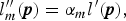
By using pseudo MEF [Reference Kinoshita, Yoshida, Shiota and Kiya19], a high-quality image is produced by fusing pseudo ME images generated from a single input image. Pseudo MEF consists of four operations: local contrast enhancement, exposure compensation, tone mapping, and MEF (see Fig. 1).
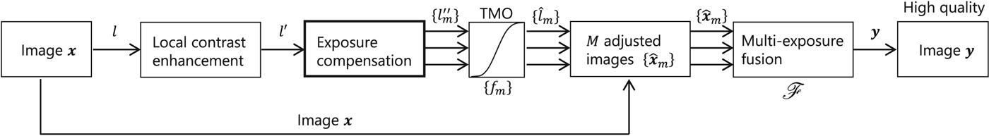
Fig. 1. Pseudo multi-exposure image fusion (MEF). Our main contributions are to propose an image segmentation method to calculate suitable parameters and to propose a novel exposure compensation method based on the segmentation method.
1) Local contrast enhancement
To enhance the local contrast of an input image x, the dodging and burning algorithm is used [Reference Youngquing, Fan and Brost24]. The luminance l′ enhanced by the algorithm is given by
 $$ l^{\prime} ({\bi p}) = \displaystyle{l({\bi p})^2 \over \bar{l} ({\bi p})},$$
where l (p) is the luminance of x and  $\bar{l} ({\bi p})$ is the local average of luminance l (p) around pixel p. It is obtained by applying a bilateral filter to l (p):
 $$ \bar{l} ({\bi p}) = \displaystyle{\sum_{{\bi p}^{\prime} \in {P}} l ({\bi p}^{\prime}) g_{\sigma_1}(\left\Vert {\bi p}^{\prime} - {\bi p} \right\Vert) g_{\sigma_2}(l ({\bi p}^{\prime}) - l ({\bi p})) \over \sum_{{\bi p}^{\prime} \in {P}} g_{\sigma_1}(\left\Vert {\bi p}^{\prime} - {\bi p} \right\Vert) g_{\sigma_2}(l ({\bi p}^{\prime}) - l ({\bi p}))},$$
where g σ (t) is a Gaussian function given by
 $$g_\sigma(t) = \exp \left( -\displaystyle{t^2 \over 2\sigma^2} \right) \, {\rm for} \, t \in {\open R}.$$
2) Exposure compensation
In the exposure-compensation step, ME images are artificially generated from a single image. To generate high-quality images by fusing these pseudo ME ones, the ME ones should clearly represent bright, middle, and dark areas in a scene. This can be achieved by adjusting the luminance l′ with multiple scale factors. A set {l″1, l″2, …, l″M} of scaled luminance is simply obtained by
 $$ l_m^{\prime\prime} ({\bi p}) = \alpha_m l^{\prime} ({\bi p}),$$
where the mth scale factor αm indicates the degree of adjustment for the mth scaled luminance l m″.
Note that how the number M of pseudo ME images is determined and how the appropriate parameter αm is estimated have never been discussed.
3) Tone mapping
Since the scaled luminance value  $l_m^{\prime\prime} ({\bi p})$ often exceeds the maximum value of common image formats, pixel values might be lost due to truncation of the values. To overcome the problem, a tone mapping operation is used to fit the range of luminance values into the interval [0, 1].
The luminance  $\hat{l}_m ({\bi p})$ of a pseudo ME image is obtained by applying a tone mapping operator f m to
  $l_m^{\prime\prime} ({\bi p})$:
 $$\hat{l}_m ({\bi p}) = f_m(l_m^{\prime\prime} ({\bi p})).$$
Reinhard's global operator is used here as a tone mapping operator f m [Reference Reinhard, Stark, Shirley and Ferwerda25].
Reinhard's global operator is given by
 $$f_m(t) = \displaystyle{t \over 1 + t}\left(1 + \displaystyle{t \over L^2_m} \right) \quad {\rm for} \ t \in [0, \infty),$$
where parameter L m > 0 determines the value of t as f m(t) = 1. Since Reinhard's global operator f m is a monotonically increasing function, truncation of the luminance values can be prevented by setting L m for  $\max l_m^{\prime\prime} ({\bi p})$.
Combining  $\hat{l}_m$, an input image x, and its luminance l, we obtain the pseudo ME images
  $\hat{\bi x}_m$:
 $$\hat{{\bi x}}_m ({\bi p}) = \displaystyle{\hat{l}_m ({\bi p}) \over l ({\bi p})} {\bi x} ({\bi p}).$$
4) Fusion of pseudo ME images
Generated pseudo ME images  ${\hat{\bi x}_m}$ can be used as input for any existing MEF methods [Reference Mertens, Kautz and Van Reeth11,Reference Nejati, Karimi, Soroushmehr, Karimi, Samavi and Najarian26]. A final image y is produced:
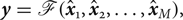 $$ {\bi y} = {\cal F}( \hat{{\bi x}}_1, \hat{{\bi x}}_2, \ldots, \hat{{\bi x}}_M),$$
where  ${\cal F} ({\bi x}_1, {\bi x}_2, \ldots, {\bi x}_M)$ indicates a function for fusing M images
  ${\bi x}_1, {\bi x}_2, \ldots, {\bi x}_M$ into a single image.
C) Scenario
Kinoshita et al. [Reference Kinoshita, Yoshida, Shiota and Kiya19] pointed out that it is effective for image enhancement to generate pseudo ME images. To produce high-quality images from pseudo ME ones, ME ones that clearly represent the whole area of a scene are required. However, the following aspects of exposure compensation have never been discussed.
• Determining the number of pseudo ME images.
• Estimating an appropriate parameter αm.
Thus, we focus on exposure compensation as shown in Fig. 1. In this paper, there are two main contributions. The first is to propose a novel image-segmentation method based on the luminance distribution of an image. The second is to propose a novel exposure compensation that uses the segmentation method. The novel compensation enables us not only to determine the number of pseudo ME images but also to estimate parameter αm.
III. PROPOSED IMAGE SEGMENTATION AND EXPOSURE COMPENSATION
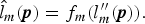
The goal of the proposed segmentation is to separate an image into M areas P 1, …, P M ⊂ P, where each of them has a specific brightness range of the image and satisfies  ${P}_1 \cup {P}_2 \cup \cdots \cup {P}_M = {P}$ (see Fig. 2). By using these results, pseudo ME images, where the mth image clearly represents area P m, are generated.
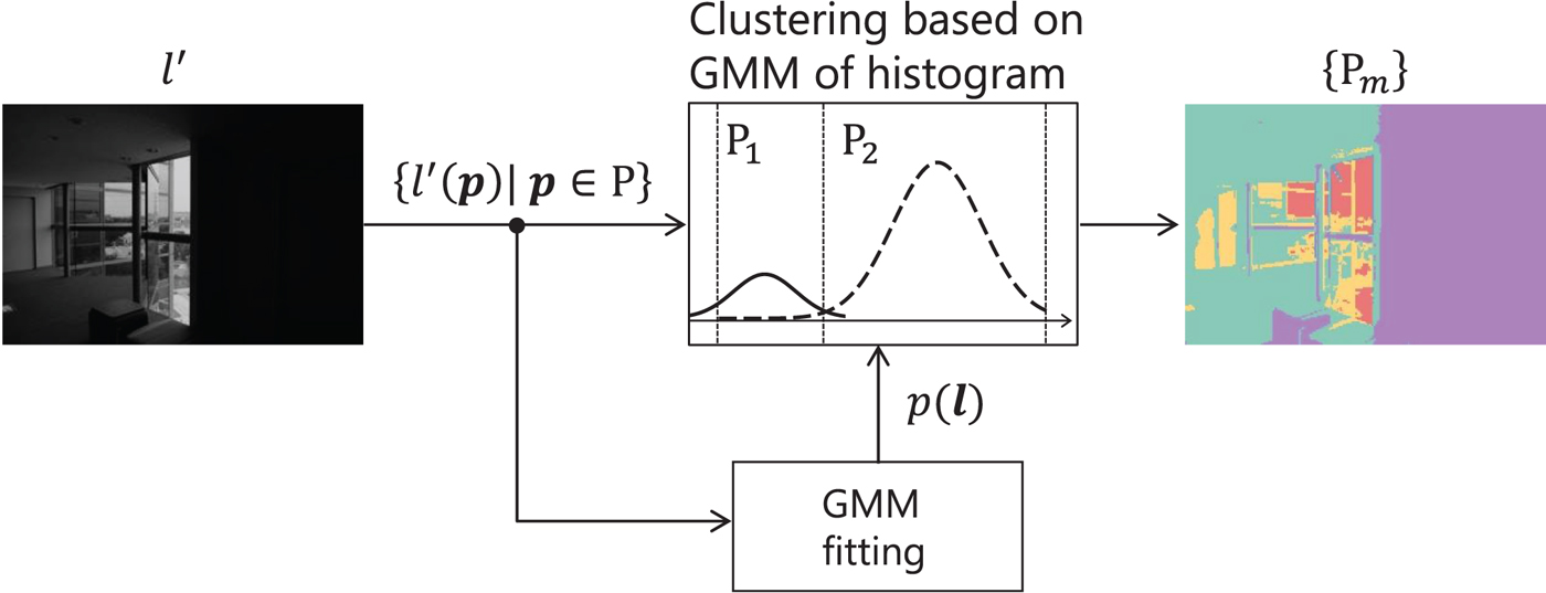
Fig. 2. Proposed image segmentation. Each separated area P m is color-coded in the right image. Separated areas {P m} are given by the GMM-based clustering method, where GMM is fit by using luminance distribution of input image I.
A) Image segmentation based on luminance distribution
The proposed segmentation method differs from typical segmentation ones in two ways.
• Drawing no attention to the structure of an image, e.g., edges.
• Allowing P m to include spatially non-contiguous regions.
For the segmentation, a Gaussian mixture distribution is utilized to model the luminance distribution of an input image. After that, pixels are classified by using a clustering algorithm based on a GMM [Reference Bishop27].
By using a GMM, the distribution of  $l^{\prime} ({\bi p})$ is given as
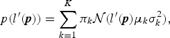 $$ p(l^{\prime} ({\bi p})) = \sum_{k=1}^K \pi_k {\cal N}({l^{\prime} ({\bi p})}{\mu_k}{\sigma_k^2}),$$
where K indicates the number of mixture components, πk is the kth mixing coefficient, and  ${\cal N} ({l^{\prime} ({\bi p})} \vert {\mu_k} {\sigma_k^2})$ is a one-dimensional Gaussian distribution with mean μk and variance μk2.
To fit the GMM into a given  $l^{\prime} ({\bi p})$, the variational Bayesian algorithm [Reference Bishop27] is utilized. Compared with the traditional maximum likelihood approach, one of the advantages is that the variational Bayesian approach can avoid overfitting even when we choose a large K. For this reason, unnecessary mixture components are automatically removed by using the approach together with a large K. K=10 is used in this paper as the maximum of the partition number M.
Here, let z be a K-dimensional binary random variable having a 1-of-K representation in which a particular element z k is equal to 1 and all other elements are equal to 0. The marginal distribution over z is specified in terms of a mixing coefficient πk, such that
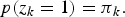 $$p(z_k = 1) = \pi_k.$$
For p(z k = 1) to be a valid probability, {πk} must satisfy
 $$0 \leq \pi_k \leq 1$$
together with
 $$\sum_{k=1}^K \pi_k = 1.$$
A cluster for an pixel p is determined by the responsibility  $\gamma (z_k \vert l^{\prime} ({\bi p}))$, which is given as a conditional probability:
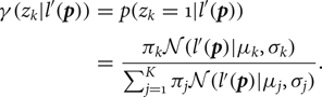 $$\eqalign{\gamma (z_k \vert l^{\prime} ({\bi p})) &= p(z_k = 1 \vert l^{\prime} ({\bi p}))\cr & = \displaystyle{\pi_k{\cal N}({l^{\prime} ({\bi p})}{\mu_k}{\sigma_k}) \over \sum_{j=1}^K \pi_j{\cal N}({l^{\prime} ({\bi p})} {\mu_j}{\sigma_j})}.}$$
When a pixel p∈P is given and m satisfies
 $$m = \mathop{\arg \max}\limits_k \gamma (z_k \vert l^{\prime} ({\bi p})),$$
the pixel p is assigned to a subset P m of P.
B) Segmentation-based exposure compensation
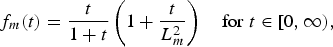
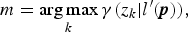
The flow of the proposed segmentation-based exposure compensation is illustrated in Fig. 3. The proposed compensation is applied to the luminance l′ after the local contrast enhancement as shown in Fig. 1. The scaled luminance l m″ is obtained according to equation (4). In the following, how to determine parameter αm is discussed.
Fig. 3. Proposed segmentation-based exposure compensation, which can automatically calculate M parameters {αm}, although conventional methods cannot. (a) Conventional [Reference Kinoshita, Yoshida, Shiota and Kiya19], (b) Proposed.
Given P m as a subset of P, the approximate brightness of P m is calculated as the geometric mean of luminance values on P m. We thus estimate an adjusted ME image  $l_m^{\prime\prime} ({\bi p})$ so that the geometric mean of its luminance equals the middle-gray of the displayed image or 0.18 on a scale from zero to one as in [Reference Reinhard, Stark, Shirley and Ferwerda25].
The geometric mean G(l|P m) of luminance l on pixel set P m is calculated using
 $$G(l\vert {P}_m) = \exp{ \left(\displaystyle{1 \over \vert {P}_m \vert} \sum_{{\bi p} \in {P}_m} \log{\left(\max{\left(l({\bi p}), \epsilon \right)}\right)} \right)},$$
where ε is set to a small value to avoid singularities at l(p) = 0.
From equation (15), parameter αm is calculated as
 $$\alpha_m = \displaystyle{0.18 \over G(l^{\prime} \vert {P}_{m})}.$$
The scaled luminance l″m, calculated by using equation (4) with parameters αm, is used as an input of the tone mapping operation described in II.B.3. As a result, we obtain M pseudo ME images.
C) Proposed procedure
The procedure for generating an enhanced image y from an input image x is summarized as follows (see Figs 1–3).
(i) Calculate luminance l from an input image x.
(ii) Local contrast enhancement: Enhance the local contrast of l by using equations (1) to (3) and then obtain the enhanced luminance l′.
(iii) Exposure compensation:
(iv) Tone mapping: Map {l″m} to
$\{\hat {l}_m\}$ according to equations (5) and (6).(v) Generate
$\{\hat {{\bi x}}_m\}$ according to equation (7).(vi) Obtain image y using the MEF method
${\cal F}$ as in equation (8).


Note that the number M satisfies 1 ≤ M ≤ K.
IV. SIMULATION
We evaluated the pseudo MEF scheme that uses the proposed segmentation-based exposure compensation in terms of the quality of enhanced images y. Hereinafter, the scheme is simply called the proposed method.
A) Comparison with conventional methods
To evaluate the quality of images produced by each of the nine methods, one of which is our own, objective quality assessments are needed. Typical quality assessments such as the peak signal to noise ratio (PSNR) and the structural similarity index (SSIM) are not suitable for this purpose because they use a target image with the highest quality as a reference. We, therefore, used statistical naturalness, which is an element of the tone mapped image quality index (TMQI) [Reference Yeganeh and Wang28], and discrete entropy to assess quality.
TMQI represents the quality of an image tone mapped from an high dynamic range (HDR) image; the index incorporates structural fidelity and statistical naturalness. Statistical naturalness is calculated without any reference images, although structural fidelity needs an HDR image as a reference. Since the process of photographing is similar to tone mapping, TMQI is also useful for evaluating photographs. In this simulation, we used only statistical naturalness for the evaluation because structural fidelity cannot be calculated without HDR images. Discrete entropy represents the amount of information in an image.
B) Simulation conditions
In the simulation, 22 photographs taken with a Canon EOS 5D Mark II camera and 16 photographs selected from an available online database [29] were used as input images x. Note that the images were taken with zero or negative exposure values (EVs). The following procedure was carried out to evaluate the effectiveness of the proposed method.
(i) Produce y from x by using the proposed method.
(ii) Compute statistical naturalness of y.
(iii) Compute discrete entropy of y.
The following nine methods were compared in this paper: HE, contrast limited adaptive histograph equalization (CLAHE) [Reference Zuiderveld and Heckbert1], adaptive gamma correction with weighting distribution (AGCWD) [Reference Huang, Cheng and Chiu2], contrast-accumulated HE (CACHE) [Reference Wu, Liu, Hiramatsu and Kashino3], low light image enhancement based on two-step noise suppression (LLIE) [Reference Su and Jung6], low-light image enhancement via illumination map estimation (LIME) [Reference Guo, Li and Ling4], simultaneous reflectance and illumination estimation (SRIE) [Reference Fu, Zeng, Huang, Zhang and Ding5], bio-inspired ME fusion framework for low-light image enhancement (BIMEF) [Reference Ying, Li and Gao21], and the proposed method. For the proposed method, Nejati's method [Reference Nejati, Karimi, Soroushmehr, Karimi, Samavi and Najarian26] was used as a fusion function  ${\cal F}$.
C) Segmentation results
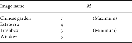
Table 1 summarizes the number of areas divided from four input images (see Figs 4 to 8) by the proposed segmentation. The minimum and maximum number of separated areas in the 38 images were three and seven, respectively. From this table, it can be seen that the proposed segmentation can avoid the overfitting of GMMs even when we utilize a large K.
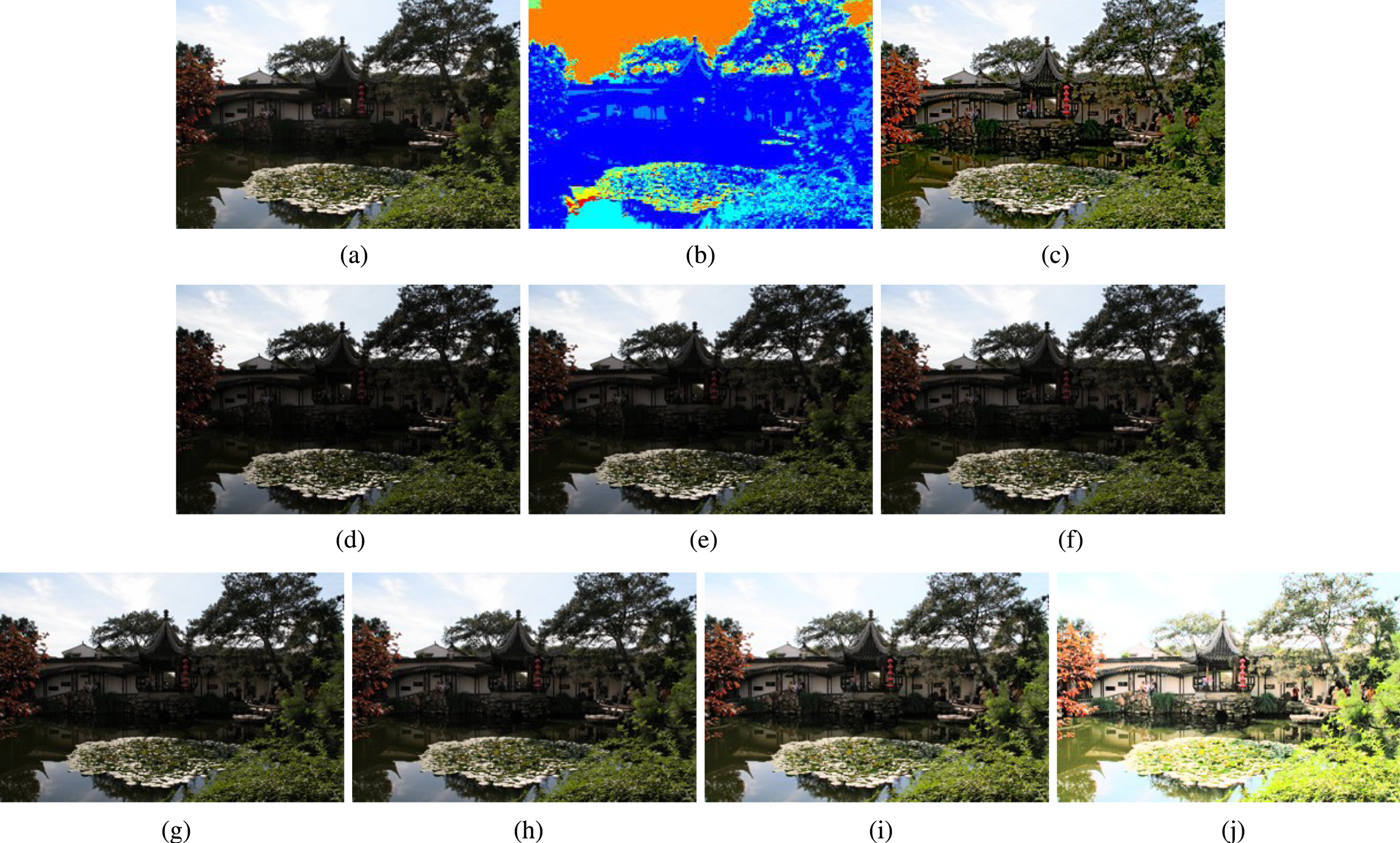
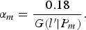
Fig. 4. Results of the proposed method (Chinese garden). (a) Input image x (0EV). Entropy: 5.767. Naturalness: 0.4786. (b) Result of the proposed segmentation, separated areas {P m} (M=7,K=10). (c) Final enhanced result of the proposed method, fused image y. Entropy: 6.510. Naturalness: 0.1774. (d–j) Adjusted images ( $\hat{\bi x}_1$,
  $\hat{{\bi x}}_2$,
  $\hat{{\bi x}}_3$,
  $\hat{{\bi x}}_4$,
  $\hat{\bi x}_5$,
  $\hat{\bi x}_6$,
  $\hat{\bi x}_7$, respectively) produced by the proposed segmentation-based exposure compensation. In (b) each color indicates area.
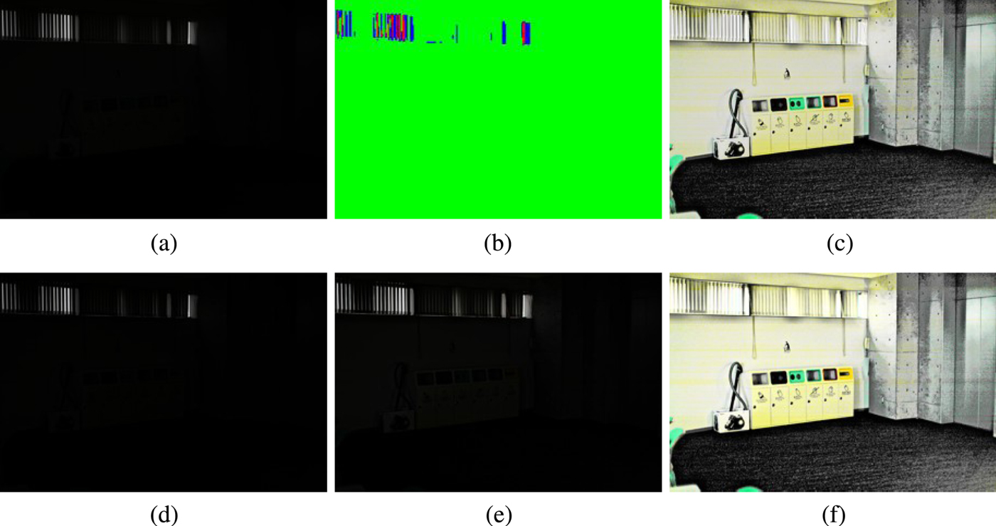
Fig. 5. Results of the proposed method (Trashbox). (a) Input image x (−6EV). Entropy: 0.249. Naturalness: 0.0000. (b) Result of the proposed segmentation, separated areas {P m} (M=3,K=10). (c) Final enhanced result of the proposed method, fused image y. Entropy: 6.830. Naturalness: 0.4886. (d–f) Adjusted images ( $\hat{\bi x}_1$,
  $\hat{\bi x}_2$,
  $\hat{\bi x}_3$, respectively) produced by the proposed segmentation-based exposure compensation. In (b), each color indicates area.
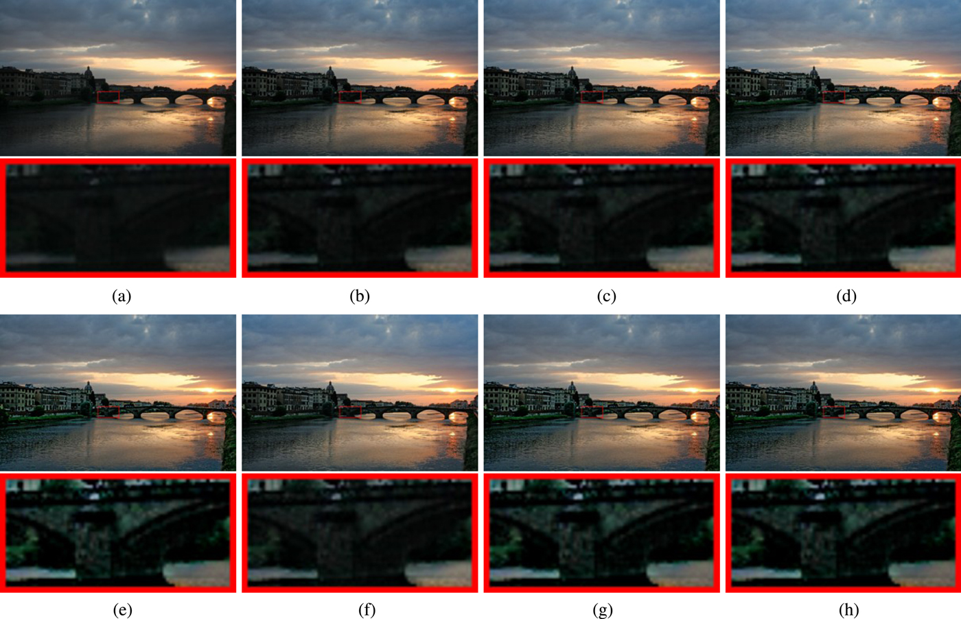
Fig. 6. Results under the use of fixed parameters M and αm (Arno). (a) Input image x (−0EV). Entropy: 6.441. Naturalness: 0.1996. (b): enhanced results with fixed M and αm, fixed M=3 and {αm} = { − 2, 0, 2}. Entropy: 6.597. Naturalness: 0.3952. (c) Fixed M=5 and {αm} = { − 4, − 2, 0, 2, 4}. Entropy: 6.745. Naturalness: 0.5430. (d): Fixed M=7 and {αm} = { − 8, − 4, …, 4, 8}. Entropy: 6.851. Naturalness: 0.6812.), (e) Enhanced result of the proposed method (M=5,K=10). Entropy: 6.640. Naturalness: 0.6693. (f): enhanced results with fixed M. Fixed M= 3. Entropy: 6.787.Naturalness: 0.6555. (g) Fixed M=5. Entropy: 6.614.]DIFdelland Naturalness: 0.6615. (h) Fixed M=7. Entropy: 6.542. Naturalness: 0.5861. Zoom-in of the boxed region is shown in bottom of each image.
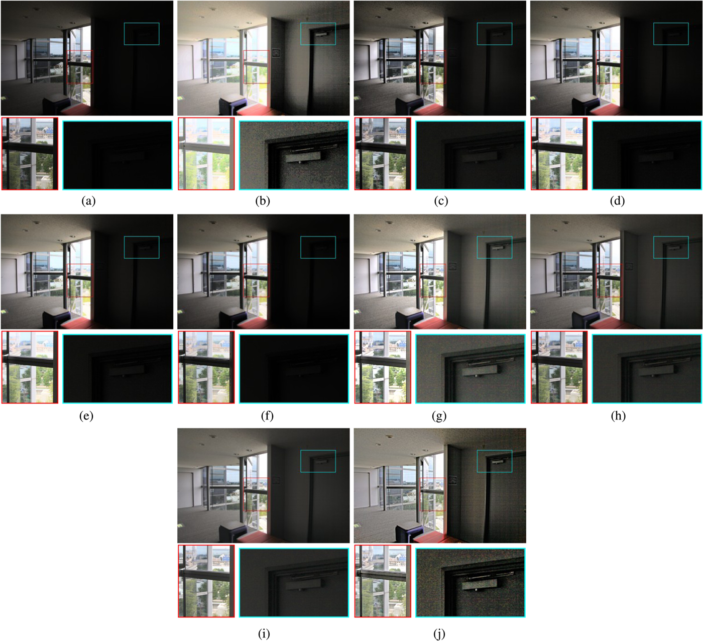
Fig. 7. Comparison of the proposed method with image-enhancement methods (Window). Zoom-ins of boxed regions are shown in bottom of each image. The proposed method can produce clear images without under- or over-enhancement. (a) Input image x (−1EV). Entropy: 3.811. Naturalness: 0.0058. (b) HE. Entropy: 5.636. Naturalness: 0.6317. (c) CLAHE [Reference Zuiderveld and Heckbert1]. Entropy: 5.040. Naturalness: 0.0945. (d) AGCWD [Reference Huang, Cheng and Chiu2]. Entropy: 5.158. Naturalness: 0.1544. (e) CACHE [Reference Wu, Liu, Hiramatsu and Kashino3]. Entropy: 5.350. Naturalness: 0.1810. (f) LLIE [Reference Su and Jung6]. Entropy: 4.730. Naturalness: 0.0608. (g) LIME [Reference Guo, Li and Ling4]. Entropy: 7.094. Naturalness: 0.9284. (h) SRIE [Reference Fu, Zeng, Huang, Zhang and Ding5]. Entropy: 5.950. Naturalness: 0.2548. (i) BIMEF [Reference Ying, Li and Gao21]. Entropy: 5.967. Naturalness: 0.2181. (j) Proposed. Entropy: 6.652. Naturalness: 0.7761.
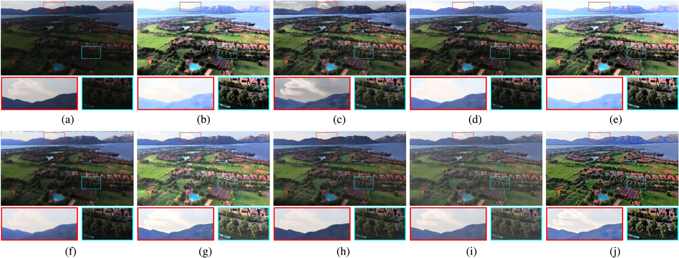
Fig. 8. Comparison of the proposed method with image-enhancement methods (Estate rsa). Zoom-ins of boxed regions are shown in the bottom of each image. The proposed method can produce clear images without under- or over-enhancement. (a) Input image x (−1.3EV). Entropy: 4.288. Naturalness: 0.0139. (b) HE. Entropy: 6.985. Naturalness: 0.7377. (c) CLAHE [Reference Zuiderveld and Heckbert1]. Entropy: 6.275 and Naturalness: 0.4578. (d) AGCWD [Reference Huang, Cheng and Chiu2]. Entropy: 6.114. Naturalness: 0.4039. (e) CACHE [Reference Wu, Liu, Hiramatsu and Kashino3]. Entropy: 7.469. Naturalness: 0.7573. (f) LLIE [Reference Su and Jung6]. Entropy: 5.807. Naturalness: 0.2314. (g) LIME [Reference Guo, Li and Ling4]. Entropy: 7.329. Naturalness: 0.8277. (h) SRIE [Reference Fu, Zeng, Huang, Zhang and Ding5]. Entropy: 5.951. Naturalness: 0.3488. (i) BIMEF [Reference Ying, Li and Gao21]. Entropy: 6.408. Naturalness: 0.6757. (j) Proposed. Entropy: 6.749. Naturalness: 0.6287.
Table 1. Examples of number M of areas {P m} separated by the proposed segmentation (K = 10)
Figures 4 and 5 illustrate example images having the maximum and minimum number of areas separated by the proposed segmentation, respectively. These results denote that an input image whose luminance values are distributed in a narrow range is divided into a few areas as in Fig. 4. In addition, a comparison between Figs 4(a) and 4(b) (and Figs 5(a) and 5(b)) shows that the proposed segmentation can separate an image into numerous areas in accordance with luminance values, where each area has a specific brightness range. As a result, the proposed segmentation-based exposure compensation works well as shown in Figs 4(d)–(j) (and Figs 5(d)–(f)), and high-quality images can be produced by fusing these adjusted images (see Figs 4(c) and 5(c)).
Figure 6 shows fused images y under the use of fixed M and αm, where (a) an input image, (b)–(d) enhanced results with fixed M and αm, (e) the enhanced result of the proposed method, and (f)–(h) enhanced results with fixed M and estimated αm by equation (16). Here, the k-means algorithm was utilized in (f)–(h) to segment images with fixed M. From Fig. 6(b)–(d), it is shown that the use of larger M is effective to produce more clear images when both M and αm are fixed. However, when a small M is used, the effect of enhancement is very small since dark/bright areas in input images are still dark/bright in enhanced images. This is because the luminance of pseudo ME images directly depends on the luminance of input images if αm is fixed.
When only M is fixed, details in images become more clear than that when both M and αm are fixed as shown in Figs 6(b) and 6(f). Hence, estimating αm adaptively for each segmented region is effective. Comparing M=3 with M=5, the enhanced image with M=5 has more clear details than that with M=3 (see Figs 6(f) and 6(g)). In addition, the enhanced image with M=5 is almost the same as that with M=7 (see Figs 6(g) and 6(h)). Therefore, it is needed to choose an appropriate M, even when αm is estimated.
The proposed method automatically determines both M and αm. The enhanced image by the proposed method is sufficiently clear as shown in Fig. 6(e). Therefore, the proposed automatic exposure compensation is effective for image enhancement.
D) Enhancement results
Enhanced images from the input image “window” are shown in Fig. 7. This figure shows that the proposed method strongly enhanced the details in dark areas. Conventional enhancement methods such as CLAHE, AGCWD, CACHE, LLIE, and BIMEF have certain effects for enhancement. However, these effects are not sufficient for visualizing areas of shadow. In addition, the proposed method can improve the quality of images without details in highlight areas being lost, i.e., over-enhancement, while the loss often occurs with conventional methods including HE and LIME. A similar trend to Fig. 7 is shown in Fig. 8. The results indicate that the proposed method enables us not only to enhance the details in dark areas but also to clearly keep the details in bright areas.
Figures 9 and 10 summarize scores for the 38 input images in terms of discrete entropy and statistical naturalness as box plots. The boxes span from the first to the third quartile, referred to as Q 1 and Q 3, and the whiskers show the maximum and minimum values in the range of [Q 1 − 1.5(Q 3 − Q 1), Q 3 + 1.5(Q 3 − Q 1)]. The band inside the box indicates the median, i.e., the second quartile Q 2. For each score (discrete entropy ∈ [0, 8], and statistical naturalness ∈ [0, 1]) a larger value means higher quality.
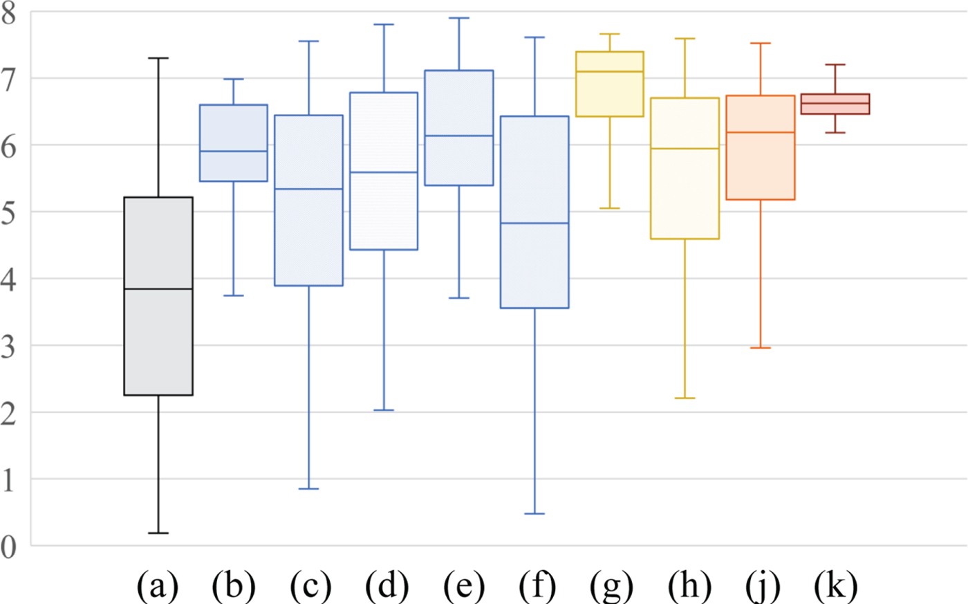
Fig. 9. Experimental results for discrete entropy. (a) Input image, (b) HE, (c) CLAHE, (d) AGCWD, (e) CACHE, (f) LLIE, (g) LIME, (h) SRIE, (i) BIMEF, and (j) Proposed. Boxes span from the first to the third quartile, referred to as Q 1 and Q 3, and whiskers show maximum and minimum values in the range of [Q 1 − 1.5(Q 3 − Q 1), Q 3 + 1.5(Q 3 − Q 1)]. Band inside box indicates median.
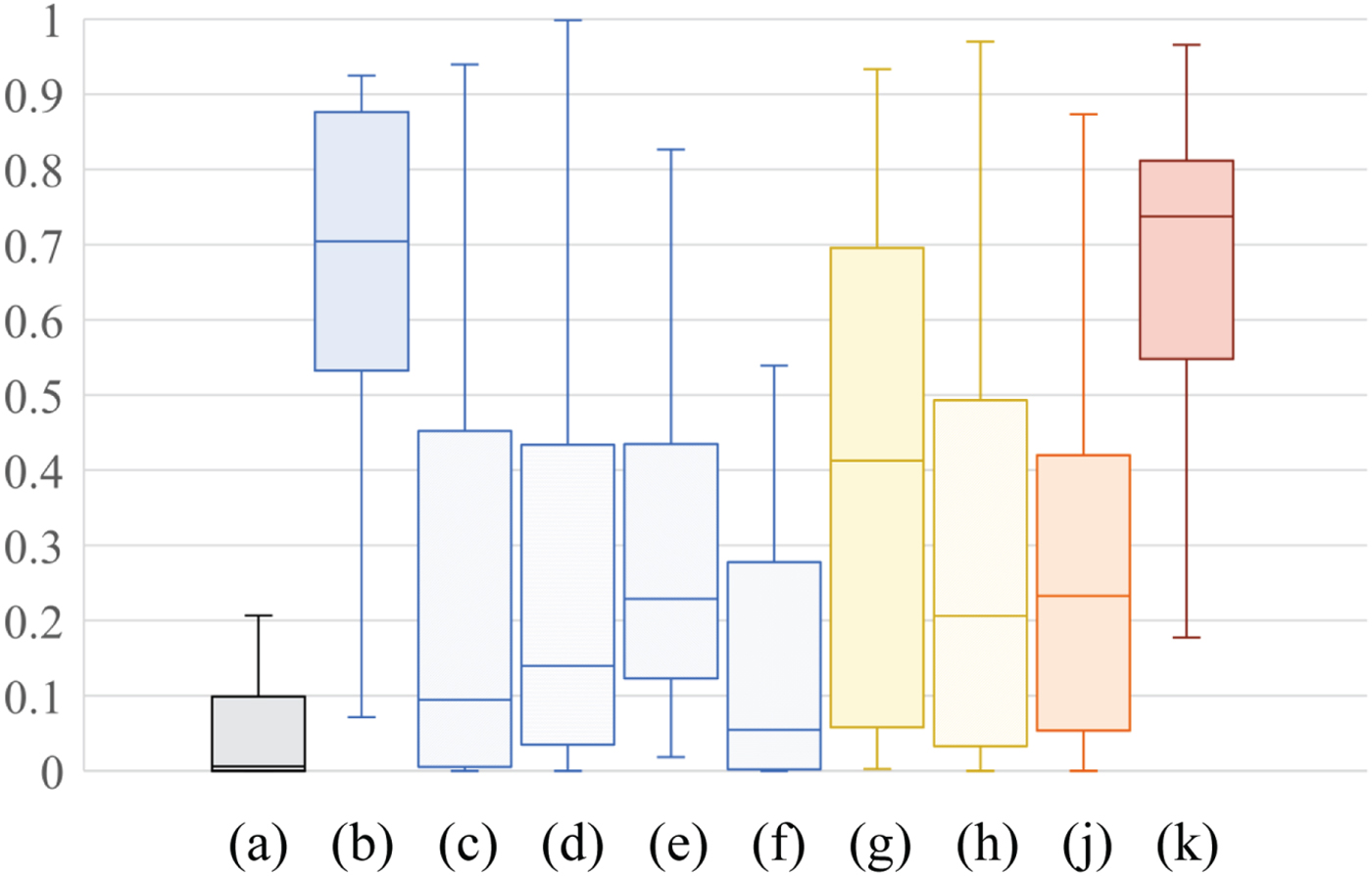
Fig. 10. Experimental results for statistical naturalness. (a) Input image, (b) HE, (c) CLAHE, (d) AGCWD, (e) CACHE, (f) LLIE, (g) LIME, (h) SRIE, (i) BIMEF, and (j) Proposed. Boxes span from the first to the third quartile, referred to as Q 1 and Q 3, and whiskers show maximum and minimum values in the range of [Q 1 − 1.5(Q 3 − Q 1), Q 3 + 1.5(Q 3 − Q 1)]. Band inside box indicates median.
In Fig. 9, it can be seen that the proposed method produced high scores that were distributed in an extremely narrow range, regardless of the scores of the input images, while LIME produced the highest median score in the nine methods. In contrast, the ranges of scores for the conventional methods were wider than that of the proposed method. Therefore, the proposed method generates high-quality images in terms of discrete entropy, compared with the conventional enhancement methods. Note that the proposed method will decrease entropy if an input image initially has a high entropy value, but an image with high entropy does not generally need to be enhanced. This is because the proposed method adjusts the luminance of the image so that the average luminance of each region is equal to the middle-gray.
Figure 10 shows that images produced by the proposed method and HE outperformed almost all images generated by the other methods including LIME. This result reflects that the proposed method and HE can strongly enhance images, as shown in Figs 7 and 8. By comparing the third quartile of the scores, HE provides the highest value in nine methods including the proposed method. In contrast, the proposed method provides the highest median and maximum value in the nine methods. For this reason, the proposed method and HE have almost the same quality in terms of statistical naturalness. In addition, the proposed method never caused a loss of details in bright areas, although HE did (see Figs 7 and 8). Therefore, the proposed method can enhance images with higher quality than HE.
For these reasons, it is confirmed that the proposed segmentation-based exposure compensation is effective for enhancing images. In addition, the pseudo MEF using exposure compensation is useful for producing high-quality images that represent both bright and dark areas.
V. CONCLUSION
In this paper, an automatic exposure-compensation method was proposed for enhancing images. For exposure compensation, a novel image-segmentation method based on luminance distribution was also proposed. The pseudo MEF scheme using the compensation one and the segmentation one enables us to produce high-quality images that well represent both bright and dark areas by fusing pseudo ME images generated from a single image. The exposure-compensation method can automatically generate pseudo ME images. In the compensation, the segmentation method is also utilized for automatic parameter setting, where the segmentation separates an image into areas by using the GMM of the luminance distribution. In experiments, image enhancement with the proposed compensation method outperformed state-of-the-art image enhancement methods in terms of both entropy and statistical naturalness. Moreover, visual comparison results showed that the proposed segmentation-based exposure compensation is effective in producing images that clearly present both bright and dark areas.
FINANCIAL SUPPORT
This work was supported by JSPS KAKENHI Grant Number JP18J20326.
STATEMENT OF INTEREST
“None.”
Yuma Kinoshita received his B.Eng. and M.Eng. degrees from Tokyo Metropolitan University, Japan, in 2016 and 2018, respectively. From 2018, he has been a Ph.D. student at Tokyo Metropolitan University. He received IEEE ISPACS Best Paper Award in 2016. His research interests are in the area of image processing. He is a student member of IEEE and IEICE.
Hitoshi Kiya received his B.E and M.E. degrees from Nagaoka University of Technology, in 1980 and 1982, respectively, and his Dr. Eng. Degree from Tokyo Metropolitan University in 1987. In 1982, he joined Tokyo Metropolitan University, where he became Full Professor in 2000. He is a Fellow of IEEE, IEICE, and ITE. He currently serves as President-Elect of APSIPA (2017–2018), and served as Inaugural Vice President (Technical Activities) of APSIPA from 2009 to 2013, Regional Director-at-Large for Region 10 of the IEEE Signal Processing Society from 2016 to 2017. He was Editorial Board Member of eight journals, including IEEE Trans. on Signal Processing, Image Processing, and Information Forensics and Security, Chair of two technical committees and Member of nine technical committees including APSIPA Image, Video, and Multimedia TC, and IEEE Information Forensics and Security TC. He was a recipient of numerous awards, including six best paper awards.


 Open access