


1. Introduction
Longevity risk management and economic valuation of insurance and pension liabilities, which have recently received considerable attention, require statistical mortality models that provide stable long-term predictions even for single populations with limited data. The Lee–Carter (LC) model (Lee-Carter, Reference Lee and Carter1992) is a basic statistical mortality model with desirable properties, wherein the log mortality is determined by the sum of a fixed age impact and a product of time index and age sensitivity.
The model fitting procedure of LC originally comprises two stages: singular value decomposition (SVD)-based dimensionality reduction of the log-mortality data and fitting of a time series model to the obtained time components. Various extensions of LC have been proposed in the literature, for example, a Poisson regression version of LC by Brouhns et al. (Reference Brouhns, Denuit and Vermunt2002), a cohort extension of LC by Renshaw and Haberman (Reference Renshaw and Haberman2006), and a two-factor period effect model by Cairns et al. (Reference Cairns, Blake and Dowd2006). Cairns et al. (Reference Cairns, Blake, Dowd, Coughlan, Epstein, Ong and Balevich2009) provides a quantitative comparison of eight stochastic mortality models including LC.
Although LC achieves good interpretability and ease of estimation using SVD and drifted random walk (RW), it has a limitation in its accuracy primarily because of two issues: incoherency between parameters because of the two-stage estimation and insufficient fitting to the nonlinearity of data.
To address the first issue, various single-stage estimations of LC in Bayesian settings, which are implemented by Markov chain Monte Carlo (MCMC) methods, have been proposed. Czado et al. (Reference Czado, Delwarde and Denuit2005) considers a single-stage Bayesian estimation of LC in a Poisson regression form and that in the state-space form was considered by Pedroza (Reference Pedroza2006), Kogure and Kurachi (Reference Kogure and Kurachi2010), Cairns et al. (Reference Cairns, Blake, Dowd, Coughlan and Khalaf-allah2011), and Fung et al. (Reference Fung, Peters and Shevchenko2017). Notable extensions of the Bayesian LC model are proposed by Kogure and Kurachi (Reference Kogure and Kurachi2010) in a risk-neutral form and Cairns et al. (Reference Cairns, Blake, Dowd, Coughlan and Khalaf-allah2011) in a multi-population form. Moreover, Fung et al. (Reference Fung, Peters and Shevchenko2017) introduces a general Bayesian state-space (BSS) modeling framework of the extensions of LC, which allows stochastic volatility in the period effect.
To address the second issue, many nonlinear extensions of LC using neural network (NN) methods have been proposed. NNs are typically defined by a network structure comprising multiple layers of neurons and an activation function that outputs a transformation of the weighted input to each neuron. As Cybenko (Reference Cybenko1989) demonstrates that any compactly supported continuous function can be uniformly approximated by a two-layer NN with a continuous sigmoidal activation function, NNs have a universal approximation capability for any function in a broad function class. The most basic NNs are feedforward NNs (FNNs) that have no cyclic connections, whereas NNs that have cyclic connections are called recurrent NNs (RNNs). NNs are also classified in supervised and unsupervised. Furthermore, convolutional NN (CNN), a sparse connected FNN to learn the neighborhood effect of the data, and RNN are often used for learning sequential data.
Richman and Wüthrich (Reference Richman and Wüthrich2021) proposes a NN-based generalization of LC using a fully connected network (FCN) with multiple hidden layers, which is called deep FCN. Perla et al. (Reference Perla, Richman, Scognamiglio and Wüthrich2021) considers many supervised NN extensions of LC and shows the superiority of one-dimensional (1D) CNN over deep FCN and long short-term memory (LSTM), a RNN suitable for learning long sequential data. Wang et al. (Reference Wang, Zhang and Zhu2021) proposes mortality forecasts using two-dimensional (2D) CNN to capture the neighborhood effect of the mortality data. Schnürch and Korn (Reference Schnürch and Korn2021) also considers 2D CNN and achieves mortality forecasts with confidence intervals. These NN approaches calibrate their models with huge training data such as the data of all countries of the Human Mortality Database (HMD; http://www.mortality.org). The huge training data will contribute to the stability and accuracy of predictions as a countermeasure to the seed robustness and overlearning problems common in NN approaches. While these NN approaches achieve single-stage estimation with relatively high prediction accuracy, they lose interpretability of the model and are not necessarily suitable for relatively small training data (e.g., single population data).
On the other hand, Hainaut (Reference Hainaut2018) proposes a replacement of SVD with an unsupervised NN for dimensionality reduction, NN-analyzer which is more commonly known as an autoencoder (AE), and Nigri et al. (Reference Nigri, Levantesi, Marino, Scognamiglio and Perla2019) proposes an application of LSTM to time components obtained from SVD, both of which have the interpretability of the model, but with the limitation of two-stage estimation. Thus, the existing NN approaches for the mortality prediction are subject to the problem of either a two-stage estimation or loss of interpretability.
To achieve a single-stage estimation of the parameters without losing interpretability, we introduce a variational AE (VAE) proposed by Kingma and Welling (Reference Kingma and Welling2013) to the mortality prediction; our method implies a fusion of NN and Bayesian approach. VAE, one of the representative generative NNs (i.e., NNs for generating new data by learning features of training data), performs the variational Bayesian estimation of the state-space model and the AE-based dimensionality reduction simultaneously.
The rest of this study is organized as follows. Section 2 discusses how the existing approaches extend the original LC model and the limitations. Section 3 presents an overview of the VAE approach. We propose a model in a generalized state-space form in Section 4 and discuss how to apply the VAE algorithm to the inference of the proposed model in Section 5. In Section 6, we apply our model to the data from the HMD and present numerical results including the calibration procedure of the model, performance comparison with LC, parameter comparison with LC to show the interpretability of the model, forecasts with confidence intervals, and remarks on the effects of changing the number of neurons in the model. Finally, Section 7 concludes this study.
2. Extensions of LC
LC defines the log-mortality rate at age
 $x$
in calendar year
$x$
in calendar year
 $t$
as follows:
$t$
as follows:
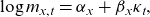 \begin{equation}\mathrm{log}\;{m}_{x,t}={\alpha }_{x}+\mathrm{}{\beta }_{x}{\kappa }_{t},\end{equation}
where
 $ \mathrm{}{\alpha }_{x}$
is the average log mortality at age
$ \mathrm{}{\alpha }_{x}$
is the average log mortality at age
 $ x$
measured over the observation period, and the bilinear term
$ x$
measured over the observation period, and the bilinear term
 $ {\beta }_{x}{\kappa }_{t}$
can be interpreted as the product of age-specific sensitivity factor and year-specific mortality improvement factor. The age-specific factor
$ {\beta }_{x}{\kappa }_{t}$
can be interpreted as the product of age-specific sensitivity factor and year-specific mortality improvement factor. The age-specific factor
 $ {\beta }_{x}$
and the year-specific factor
$ {\beta }_{x}$
and the year-specific factor
 $ {\kappa }_{t}$
are obtained by the SVD of the log-mortality data net of the age-specific averages {
$ {\kappa }_{t}$
are obtained by the SVD of the log-mortality data net of the age-specific averages {
 $ {\alpha}_{x}$
}
$ {\alpha}_{x}$
}
 $ ,$
where the following model identification constraints are required:
$ ,$
where the following model identification constraints are required:
 \begin{equation}\left\{\!\begin{array}{c} \sum\limits_{x}{\beta }_{x}=1\\[10pt] \sum\limits_{t}{\kappa }_{t}=0.\end{array}\right.\end{equation}
The prediction of future mortality in LC can be performed via a two-stage procedure: obtaining {
 $ {\kappa }_{t}$
} by SVD and then fitting a time series model to {
$ {\kappa }_{t}$
} by SVD and then fitting a time series model to {
 $ {\kappa }_{t}$
}. It is common to apply a drifted RW model determined by:
$ {\kappa }_{t}$
}. It is common to apply a drifted RW model determined by:
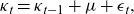 \begin{equation}{\kappa }_{t} = {\kappa }_{t-1}+\mu +{\epsilon}_{t},\end{equation}
where
 $ {\epsilon}_{t}$
follows an
$ {\epsilon}_{t}$
follows an
 $ iid$
(i.e., independent and identically distributed) standard normal distribution.
$ iid$
(i.e., independent and identically distributed) standard normal distribution.
The interpretability of LC has given rise to various extensions, for example, Renshaw and Haberman (Reference Renshaw and Haberman2006) (RH) makes a cohort extension by adding a new term
 $ {\beta'}_{\!\!x}{\kappa'}_{\!\!t-x}$
on the right-hand side of Equation (2.1).
$ {\beta'}_{\!\!x}{\kappa'}_{\!\!t-x}$
on the right-hand side of Equation (2.1).
However, LC is known to have limitations in estimation accuracy, primarily because of incoherency among variables caused by the two-stage estimation and the limitation of nonlinear representation capability of the bilinear form.
For the first issue, single-stage estimations of LC in Bayesian settings have been proposed. A direct translation of LC into a state-space form in Pedroza (Reference Pedroza2006) is given by:
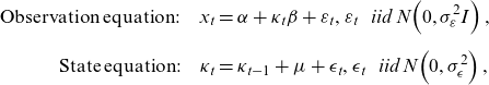 \begin{align}\mathrm{Observation\;equation}:\quad {x}_{t} & =\alpha +{\kappa}_{t}\beta +{\varepsilon }_{t},{\varepsilon }_{t}\mathrm{}\;~\;\mathrm{}iid\mathrm{}\;N\!\left(0,{\sigma }_{\varepsilon }^{2}I\right),\nonumber \\[5pt]\mathrm{State\;equation}:\quad {\kappa }_{t}&={\kappa }_{t-1}+\mu +{\epsilon}_{t},{\epsilon}_{t}\mathrm{}\;~\;\mathrm{}iid\mathrm{}\;N\!\left(0,{\sigma }_{\epsilon}^{2}\right),\end{align}
where
 ${x}_{t}={\left({\mathrm{log}\;m}_{t,0},\mathrm{log}\;{m}_{t,1},\dots ,\mathrm{log}\;{m}_{t,n}\right)}^{T}$
;
${x}_{t}={\left({\mathrm{log}\;m}_{t,0},\mathrm{log}\;{m}_{t,1},\dots ,\mathrm{log}\;{m}_{t,n}\right)}^{T}$
;
 $\alpha ={\left({\alpha }_{0},{\alpha }_{1},\dots ,{\alpha }_{n}\right)}^{T}$
;
$\alpha ={\left({\alpha }_{0},{\alpha }_{1},\dots ,{\alpha }_{n}\right)}^{T}$
;
 $\beta =({\beta }_{0},$
 ${\beta }_{1},\dots ,{\beta }_{n})^{T}$
; n denotes the maximum age observed. Here, MCMC is required to obtain posterior joint distributions for the parameters
${\beta }_{1},\dots ,{\beta }_{n})^{T}$
; n denotes the maximum age observed. Here, MCMC is required to obtain posterior joint distributions for the parameters
 $ \alpha $
,
$ \alpha $
,
 $ \beta $
,
$ \beta $
,
 $ {\sigma }_{\varepsilon }$
,
$ {\sigma }_{\varepsilon }$
,
 $ \mu $
, and
$ \mu $
, and
 $ {\sigma }_{\epsilon}$
. Because the MCMC is computationally intensive, the number of age categories to be estimated is often limited in many previous studies. Although many Bayesian extensions of LC have been proposed, they follow the bilinear form as in LC or RH, which results in limited nonlinear representation capabilities.
$ {\sigma }_{\epsilon}$
. Because the MCMC is computationally intensive, the number of age categories to be estimated is often limited in many previous studies. Although many Bayesian extensions of LC have been proposed, they follow the bilinear form as in LC or RH, which results in limited nonlinear representation capabilities.
For the second issue, the extension of the nonlinear representation capabilities, NN approaches have been recently proposed; our study is in this context. The reason behind the application of NNs to the nonlinear extension of models is the universal approximation capability of NNs that is demonstrated by Cybenko (Reference Cybenko1989). NNs generally comprise an input layer, hidden layers, an output layer, neurons in each layer, links between the neurons in different layers, and activation functions. In an FNN, the
 $ {d}_{i+1}$
-dimensional vector
$ {d}_{i+1}$
-dimensional vector
 $ {y}^{i+1}$
representing the output value of neurons in the i+1-th layer
$ {y}^{i+1}$
representing the output value of neurons in the i+1-th layer
 $ $
is determined by the
$ $
is determined by the
 $ {d}_{i}$
-dimensional output vector
$ {d}_{i}$
-dimensional output vector
 $ {y}^{i}$
in the previous layer, the activation function
$ {y}^{i}$
in the previous layer, the activation function
 $ \phi $
, the weights
$ \phi $
, the weights
 $ {W}^{i}\in {\mathbb{R}}_{{d}_{i+1}\times {d}_{i}}$
, and the bias
$ {W}^{i}\in {\mathbb{R}}_{{d}_{i+1}\times {d}_{i}}$
, and the bias
 $ {b}^{i}\in {{\mathbb{R}}_{d}}_{i+1}$
as follows:
$ {b}^{i}\in {{\mathbb{R}}_{d}}_{i+1}$
as follows:
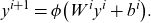 \begin{equation}{y}^{i+1}=\phi \!\left({W}^{i}{y}^{i}+{b}^{i}\right)\!.\end{equation}
NNs are trained to obtain weights
 $ {W}^{i}$
that minimize loss functions under a given network structure and activation function, typically using a gradient descent method (GDM).
$ {W}^{i}$
that minimize loss functions under a given network structure and activation function, typically using a gradient descent method (GDM).
Nigri et al. (Reference Nigri, Levantesi, Marino, Scognamiglio and Perla2019) proposes a two-stage NN extension of LC in which the LSTM was applied to the extrapolation of time series components obtained by SVD. Perla et al. (Reference Perla, Richman, Scognamiglio and Wüthrich2021) considers NN extensions of LC, which could perform single-stage estimations and demonstrates that 1D CNN outperformed FCN proposed by Richman and Wüthrich (Reference Richman and Wüthrich2021) and LSTM. CNN, proposed by LeCun et al. (Reference Lecun, Boser, Denker, Henderson, Howard, Hubbard and Jackel1990), is generally known as an effective method for 2D images and 3D spatial data; however, it has been recently used for 1D time series data. CNN replaces the product term
 $ {W}^{i}{y}^{i}$
in Equation (2.5) with the convolution, as described below; it is often performed in three stages. In the first stage, the convolution with shared weights is performed; in the second stage, the value obtained by the convolution is nonlinearly transformed by an activation function; finally, a pooling function is used to output the value. The 1D CNN uses the convolution filter
$ {W}^{i}{y}^{i}$
in Equation (2.5) with the convolution, as described below; it is often performed in three stages. In the first stage, the convolution with shared weights is performed; in the second stage, the value obtained by the convolution is nonlinearly transformed by an activation function; finally, a pooling function is used to output the value. The 1D CNN uses the convolution filter
 $ {W}^{i,j}\in {\mathbb{R}}_{d\times m}\!\left(j=1,\dots ,J\right)$
instead of the weight
$ {W}^{i,j}\in {\mathbb{R}}_{d\times m}\!\left(j=1,\dots ,J\right)$
instead of the weight
 $ {W}^{i}$
in Equation (2.5), where
$ {W}^{i}$
in Equation (2.5), where
 $ m\in \mathbb{N}$
denotes the kernel size of the filter and
$ m\in \mathbb{N}$
denotes the kernel size of the filter and
 $ J$
denotes the number of filters. Then, the output data of layer
$ J$
denotes the number of filters. Then, the output data of layer
 $ i$
,
$ i$
,
 $ {y}^{i}\in {\mathbb{R}}_{d\times T}$
, is transformed as follows:
$ {y}^{i}\in {\mathbb{R}}_{d\times T}$
, is transformed as follows:
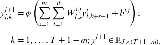 \begin{align} {y}_{j,k}^{i+1}&=\phi \left(\sum _{s=1}^{m}\sum _{l=1}^{d}{W}_{l,s}^{i,j}{y}_{l,k+s-1}^{i}+{b}^{i,j}\right);\nonumber \\[5pt] k&=1,\dots ,T+1-m;\;\mathrm{}{y}^{i+1}\in {\mathbb{R}}_{J\times \left(T+1-m\right).}\end{align}
After the above transformation, the pooling function is employed. Generally, the pooling function returns the maximum, minimum, or average value within each window region of the input data. For an h-dimensional CNN input,
 $ {y}^{i}\in {\mathbb{R}}_{d\times T}$
and
$ {y}^{i}\in {\mathbb{R}}_{d\times T}$
and
 $ {y}^{i+1}\in {\mathbb{R}}_{J\times \left(T+1-m\right)}$
are changed to
$ {y}^{i+1}\in {\mathbb{R}}_{J\times \left(T+1-m\right)}$
are changed to
 $ {y}^{i}\in {\mathbb{R}}_{h\times d\times T}$
and
$ {y}^{i}\in {\mathbb{R}}_{h\times d\times T}$
and
 $ {y}^{i+1}\in {\mathbb{R}}_{h\times J\times \left(T+1-m\right)}$
. Wang et al. (Reference Wang, Zhang and Zhu2021) proposes mortality forecasts using two-dimensional (2D) CNN to capture the neighborhood effect of the mortality data. Schnürch and Korn (Reference Schnürch and Korn2021) also considers 2D CNN and achieves mortality forecasts with confidence intervals. The confidence intervals are not based on the endogenous randomness as in the BSS models, but on the exogenous randomness driven by the random seed for the NN, which corresponds to the model uncertainty.
$ {y}^{i+1}\in {\mathbb{R}}_{h\times J\times \left(T+1-m\right)}$
. Wang et al. (Reference Wang, Zhang and Zhu2021) proposes mortality forecasts using two-dimensional (2D) CNN to capture the neighborhood effect of the mortality data. Schnürch and Korn (Reference Schnürch and Korn2021) also considers 2D CNN and achieves mortality forecasts with confidence intervals. The confidence intervals are not based on the endogenous randomness as in the BSS models, but on the exogenous randomness driven by the random seed for the NN, which corresponds to the model uncertainty.
Hainaut (Reference Hainaut2018) proposes a two-stage estimation of LC with a NN-based dimensionality reduction as an alternative to SVD. The NN algorithm called NN-analyzer in Hainaut (Reference Hainaut2018) can be classified as AE. Generally, AE is a NN that uses a low-dimensional hidden layer and learns such that the input data are close to the output of the AE reconstructed via the hidden layer and can extract nonlinear features and characterize multidimensional data in low-dimensional components. The first part of AE, which outputs low-dimensional features from the original data, is called an encoder
 $ {f}^{enc}$
, and the second part, which reconstructs data from low-dimensional features, is called a decoder
$ {f}^{enc}$
, and the second part, which reconstructs data from low-dimensional features, is called a decoder
 $ {f}^{dec}$
.
$ {f}^{dec}$
.
For the input data
 $ X\!\left(t\right)$
at time
$ X\!\left(t\right)$
at time
 $ t$
given by a vector of age-specific log-mortality rates net of the age-specific averages, the reconstructed data
$ t$
given by a vector of age-specific log-mortality rates net of the age-specific averages, the reconstructed data
 $ \widehat{X}\!\left(t\right)$
by
$ \widehat{X}\!\left(t\right)$
by
 $ {f}^{dec}$
and the d-dimensional latent factor
$ {f}^{dec}$
and the d-dimensional latent factor
 $ {\kappa }_{t}^{nn}=\left({\kappa }_{t}^{nn,1},\dots ,{\kappa }_{t}^{nn,d}\right)$
, the NN-analyzer is described as follows:
$ {\kappa }_{t}^{nn}=\left({\kappa }_{t}^{nn,1},\dots ,{\kappa }_{t}^{nn,d}\right)$
, the NN-analyzer is described as follows:
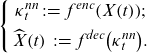 \begin{equation}\left\{\begin{array}{c}{\kappa }_{t}^{nn}\;:\!=\;{f}^{enc}\!\left(X\!\left(t\right)\right)\!;\\[5pt] \widehat{X}\!\left(t\right)\;:\!=\;{f}^{dec}\!\left({\kappa }_{t}^{nn}\right)\!.\end{array}\right.\end{equation}
The loss function is given by the squared error between
 $ \widehat{X}\!\left(t\right)$
and
$ \widehat{X}\!\left(t\right)$
and
 $ X\!\left(t\right)$
, and the parameters of
$ X\!\left(t\right)$
, and the parameters of
 $ {f}^{enc}$
and
$ {f}^{enc}$
and
 $ {f}^{dec}$
are estimated using a GDM to minimize the loss function.
$ {f}^{dec}$
are estimated using a GDM to minimize the loss function.
Moreover, the NN analyzer has the following features:
-
It has a symmetric network structure with three hidden layers using hyperbolic tangent sigmoidal and identity function as activation functions for both
 $ {f}^{enc}$
and
$ {f}^{dec}$
.
$ {f}^{enc}$
and
$ {f}^{dec}$
. -
The input and output data are evenly divided in subgroups, and each subgroup is exclusively connected to a specific neuron in the input and output layers, resulting in a sparsely connected AE (SAE), which is expected to prevent overlearning.
-
A genetic algorithm is used to identify appropriate initial values for the GDM.


Finally, using the latent factors, the mortality model is expressed as follows:
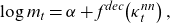 \begin{equation}\mathrm{log}\;{m}_{t}=\alpha +{f}^{dec}\!\left({\kappa }_{t}^{nn}\right),\end{equation}
where
 $ \mathrm{}{m}_{t}$
and the average mortality rate
$ \mathrm{}{m}_{t}$
and the average mortality rate
 $ \alpha $
are vectors of values for each age. The decoder term in Equation (2.8) gives a nonlinear generalization of the bilinear term of LC; however, the prediction requires extrapolating the latent factor
$ \alpha $
are vectors of values for each age. The decoder term in Equation (2.8) gives a nonlinear generalization of the bilinear term of LC; however, the prediction requires extrapolating the latent factor
 $ {\kappa }_{t}^{nn}$
by a time series model, resulting in a two-stage estimation. We introduce VAE to perform the single-stage estimation of the AE-based extension of LC. For more theoretical background on NNs and AEs, we refer to Wüthrich and Merz (2022).
$ {\kappa }_{t}^{nn}$
by a time series model, resulting in a two-stage estimation. We introduce VAE to perform the single-stage estimation of the AE-based extension of LC. For more theoretical background on NNs and AEs, we refer to Wüthrich and Merz (2022).
3. Variational autoencoder (VAE)
VAE, proposed by Kingma and Welling (Reference Kingma and Welling2013), is a type of deep generative model with an AE structure that performs unsupervised learning with dimensionality reduction to a latent space. VAE assumes a probability distribution for the latent space, unlike the conventional AE, and can be implemented without using MCMC techniques. The aim of VAE is to identify
 $ {p}_{\theta }\!\left(x\right)$
that denotes the generative distribution of the data
$ {p}_{\theta }\!\left(x\right)$
that denotes the generative distribution of the data
 $x\;\mathrm{with\;generative\;parameter}\;\theta$
; in the process, it can acquire the dimensionally reduced latent representation of data as a probability distribution. Assume that, for T
$x\;\mathrm{with\;generative\;parameter}\;\theta$
; in the process, it can acquire the dimensionally reduced latent representation of data as a probability distribution. Assume that, for T
 $ \in \mathbb{N}$
, there exists a set of latent variables
$ \in \mathbb{N}$
, there exists a set of latent variables
 $ Z={\left\{{z}_{t}\right\}}_{t=1}^{T}$
that generates a sample dataset
$ Z={\left\{{z}_{t}\right\}}_{t=1}^{T}$
that generates a sample dataset
 $ X={\left\{{x}_{t}\right\}}_{t=1}^{T}$
with probability
$ X={\left\{{x}_{t}\right\}}_{t=1}^{T}$
with probability
 $ {p}_{\theta }\!\left({x}_{t}|{z}_{t}\right)$
for each
$ {p}_{\theta }\!\left({x}_{t}|{z}_{t}\right)$
for each
 $ t$
, and
$ t$
, and
 $ \mathrm{}{z}_{t}$
follows the prior distribution
$ \mathrm{}{z}_{t}$
follows the prior distribution
 $ {p}_{\theta }\!\left({z}_{t}\right),$
where
$ {p}_{\theta }\!\left({z}_{t}\right),$
where
 $ {p}_{\theta }\!\left({z}_{t}\right)$
and
$ {p}_{\theta }\!\left({z}_{t}\right)$
and
 $ {p}_{\theta }\!\left({x}_{t}\right|{z}_{t})$
follow probability distributions differentiable with respect to the parameters to be identified.
$ {p}_{\theta }\!\left({x}_{t}\right|{z}_{t})$
follow probability distributions differentiable with respect to the parameters to be identified.
Because it is generally difficult to directly estimate the multidimensional posterior distribution
 $ {p}_{\theta }\!\left(Z|X\right),$
a variational approximation with the parameter
$ {p}_{\theta }\!\left(Z|X\right),$
a variational approximation with the parameter
 $\varphi,$
 $ {q}_{\varphi }\!\left(Z|X\right),$
is used; the approximation is often implemented in the form of a mean field approximation via a factor decomposable distribution as follows:
$ {q}_{\varphi }\!\left(Z|X\right),$
is used; the approximation is often implemented in the form of a mean field approximation via a factor decomposable distribution as follows:
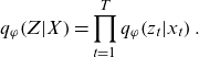 \begin{equation}{q}_{\varphi }\!\left(Z|X\right)=\prod _{t=1}^{T}{q}_{\varphi }\!\left({z}_{t}|{x}_{t}\right).\end{equation}
From the AE perspective, the approximate distribution
 $ {q}_{\varphi }\!\left({z}_{t}|{x}_{t}\right)$
and generative distribution
$ {q}_{\varphi }\!\left({z}_{t}|{x}_{t}\right)$
and generative distribution
 $ {p}_{\theta }\!\left({x}_{t}\right|{z}_{t})$
are considered probabilistic encoder and decoder, respectively. The generative parameter
$ {p}_{\theta }\!\left({x}_{t}\right|{z}_{t})$
are considered probabilistic encoder and decoder, respectively. The generative parameter
 $ \theta $
and variational parameter
$ \theta $
and variational parameter
 $ \varphi $
are learned as network parameters in VAE to maximize the evidence lower bound (ELBO) given by Equation (3.2). The meanings of the ELBO become clear by rewriting Equation (3.2) with the Kullback–Leibler (KL) divergence represented by
$ \varphi $
are learned as network parameters in VAE to maximize the evidence lower bound (ELBO) given by Equation (3.2). The meanings of the ELBO become clear by rewriting Equation (3.2) with the Kullback–Leibler (KL) divergence represented by
 $ {D}_{KL}\!\left[\left|\right|\right],$
which gives asymmetric distances between distributions, as shown in Equations (3.3) and (3.4). We also refer to Section 11.6.3 of Wüthrich and Merz (2022) for more details:
$ {D}_{KL}\!\left[\left|\right|\right],$
which gives asymmetric distances between distributions, as shown in Equations (3.3) and (3.4). We also refer to Section 11.6.3 of Wüthrich and Merz (2022) for more details:
 \begin{equation}\mathrm{E}\mathrm{L}\mathrm{B}\mathrm{O}={\int }_{}^{}{q}_{\varphi }\!\left(Z\right|\!X)\mathrm{log}\frac{{p}_{\theta }(Z,X)}{{q}_{\varphi }\!\left(\!Z\right|\!X\!)}dZ.\end{equation}
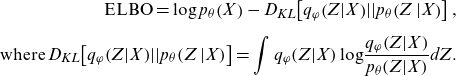 \begin{equation}\begin{split}\mathrm{E}\mathrm{L}\mathrm{B}\mathrm{O}=\mathrm{log}\;{p}_{\theta }\!\left(X\right)-{D}_{KL}\!\left[{q}_{\varphi }\!\left(Z\right|\!X\!\left)\right|\!\left|{p}_{\theta }\right(\!Z\left|X\right)\right],\\[5pt]\mathrm{where}\; {D}_{KL}\!\left[{q}_{\varphi }\!\left(Z\right|\!X\!\left)\right|\!\left|{p}_{\theta }\right(\!Z\left|X\right)\right]=\int {q}_{\varphi }\!\left(Z|X\right)\mathrm{log}\frac{{q}_{\varphi }\!\left(Z|X\right)}{{p}_{\theta }\!\left(Z|X\right)}dZ.\end{split}\end{equation}
 \begin{equation}\begin{split}\mathrm{E}\mathrm{L}\mathrm{B}\mathrm{O}=\int {q}_{\varphi }\!\left(Z|X\right)\mathrm{log}\;{p}_{\theta }\!\left(X|Z\right)dZ-{D}_{KL}\!\left[{q}_{\varphi }\!\left(Z\right|\!X\!\left)\right|\!\left|{p}_{\theta }\right(\!Z)\right],\\[5pt]\mathrm{where}\; {D}_{KL}\!\left[{q}_{\varphi }\!\left(Z\right|\!X\!\left)\right|\!\left|{p}_{\theta }\right(\!Z)\right]=\int {q}_{\varphi }\!\left(Z\right|\!X)\mathrm{log}\frac{{q}_{\varphi }\!\left(Z\right|\!X)}{{p}_{\theta }\!\left(Z\right)}dZ.\end{split}\end{equation}
Equation (3.3) shows that the ELBO maximization implies maximizing the log-likelihood of the data with penalizing the approximation error given by
 $ {D}_{KL}\!\left[{q}_{\varphi }\!\left(Z\right|\!X\!\left)\right|\left|{p}_{\theta }\right(\!Z\!\left|X\right)\right].$
From the perspective of AE, Equation (3.4) shows that the integral term of the ELBO indicates an expected value of the negative reconstruction error of the data
$ {D}_{KL}\!\left[{q}_{\varphi }\!\left(Z\right|\!X\!\left)\right|\left|{p}_{\theta }\right(\!Z\!\left|X\right)\right].$
From the perspective of AE, Equation (3.4) shows that the integral term of the ELBO indicates an expected value of the negative reconstruction error of the data
 $ $
by the decoder
$ $
by the decoder
 $ {p}_{\theta }\!\left(X|Z\right)$
because
$ {p}_{\theta }\!\left(X|Z\right)$
because
 $ \mathrm{log}\;{p}_{\theta }\!\left(X|Z\right)$
is closer to 0 for higher reconstruction probability and takes a greater negative value for lower reconstruction probability; the second (KL) term of the ELBO acts as a regularizer that penalizes the KL distance between the approximate posterior distribution
$ \mathrm{log}\;{p}_{\theta }\!\left(X|Z\right)$
is closer to 0 for higher reconstruction probability and takes a greater negative value for lower reconstruction probability; the second (KL) term of the ELBO acts as a regularizer that penalizes the KL distance between the approximate posterior distribution
 $ {q}_{\varphi }\!\left(Z|X\right)$
and the prior distribution
$ {q}_{\varphi }\!\left(Z|X\right)$
and the prior distribution
 $ {p}_{\theta }\!\left(Z\right)$
. Thus, the ELBO maximization simultaneously performs the data reconstruction error minimization, which is essential for AEs, and regularization. While the distributions are usually selected such that the KL term of Equation (3.4) can be analytically calculated, the first term is difficult to analytically calculate. Thus, a sampling approximation by
$ {p}_{\theta }\!\left(Z\right)$
. Thus, the ELBO maximization simultaneously performs the data reconstruction error minimization, which is essential for AEs, and regularization. While the distributions are usually selected such that the KL term of Equation (3.4) can be analytically calculated, the first term is difficult to analytically calculate. Thus, a sampling approximation by
 $ {z}_{t}$
following
$ {z}_{t}$
following
 $ {q}_{\varphi }\!\left({z}_{t}|{x}_{t}\right)$
and a reparameterization technique (called reparameterization trick) for
$ {q}_{\varphi }\!\left({z}_{t}|{x}_{t}\right)$
and a reparameterization technique (called reparameterization trick) for
 $ {z}_{t}$
are required to optimize parameters using the GDM. The reparameterization is determined by a differentiable bivariate function of the data point
$ {z}_{t}$
are required to optimize parameters using the GDM. The reparameterization is determined by a differentiable bivariate function of the data point
 $ {x}_{t}$
and an auxiliary noise variable
$ {x}_{t}$
and an auxiliary noise variable
 $ {\epsilon}_{t}$
as follows:
$ {\epsilon}_{t}$
as follows:
 \begin{equation}{z}_{t}={g}_{\varphi }\!\left({x}_{t},{\epsilon}_{t}\right).\end{equation}
In particular, assuming that the
 $ iid$
noise
$ iid$
noise
 $ {\epsilon}_{t}$
follows standard normal distribution,
$ {\epsilon}_{t}$
follows standard normal distribution,
 $ {g}_{\varphi }\!\left({x}_{t},{\epsilon}_{t}\right)$
can be expressed as follows:
$ {g}_{\varphi }\!\left({x}_{t},{\epsilon}_{t}\right)$
can be expressed as follows:
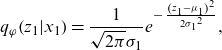
 \begin{align}{g}_{\varphi }\!\left({x}_{t},{\epsilon}_{t}\right)&={\mu }_{t}+{\sigma }_{t}{\epsilon}_{t};\nonumber \\[5pt] \left({\mu }_{t},{\sigma }_{t}\right)&={f}_{\varphi }^{enc}\!\left({x}_{t}\right),\end{align}
where the parameters are given by a vector-valued function
 $ {f}_{\varphi }^{enc}\!\left({x}_{t}\right)$
in the encoder.
$ {f}_{\varphi }^{enc}\!\left({x}_{t}\right)$
in the encoder.
For
 $ L\in \mathbb{N}$
denoting the number of samples from
$ L\in \mathbb{N}$
denoting the number of samples from
 $ {g}_{\varphi }\!\left({x}_{t},{\epsilon}_{t}\right)$
, the sampling approximation of the first term is given by:
$ {g}_{\varphi }\!\left({x}_{t},{\epsilon}_{t}\right)$
, the sampling approximation of the first term is given by:
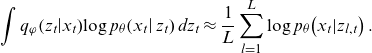 \begin{equation}\int {q}_{\varphi }\!\left({z}_{t}\right|\!{x}_{t})\mathrm{log}\;{p}_{\theta }\!\left({x}_{t}\right|{z}_{t})\;d{z}_{t}\approx \frac{1}{L}\sum _{l=1}^{L}\mathrm{log}\;p_{\theta}\! \left({x}_{t}|{z}_{l,t}\right).\end{equation}
4. The model
We propose a nonlinear extension of LC, written as a state-space model with a latent variable that follows a drifted RW process. For the data
 $ {\left\{{x}_{t}\right\}}_{t=1}^{T}$
comprising vectors of age-specific log-mortality rates for each observation year
$ {\left\{{x}_{t}\right\}}_{t=1}^{T}$
comprising vectors of age-specific log-mortality rates for each observation year
 $ t$
and latent variables
$ t$
and latent variables
 $ {\left\{{z}_{t}\right\}}_{t=1}^{T}$
for all observation years, their joint probability and graphical representation (Figure 1) are as follows:
$ {\left\{{z}_{t}\right\}}_{t=1}^{T}$
for all observation years, their joint probability and graphical representation (Figure 1) are as follows:
 \begin{equation}{p}_{\theta ,\;\xi }\!\left({x}_{1},{x}_{2},\dots ,{x}_{T},{z}_{1},{z}_{2},\dots ,{z}_{T}\right)=\prod _{t=1}^{T}{p}_{\theta }\!\left({x}_{t}|{z}_{t}\right)\prod _{t=1}^{T-1}{p}_{\xi }\!\left({z}_{t+1}|{z}_{t}\right){p}_{\xi }\!\left({z}_{1}\right).\end{equation}
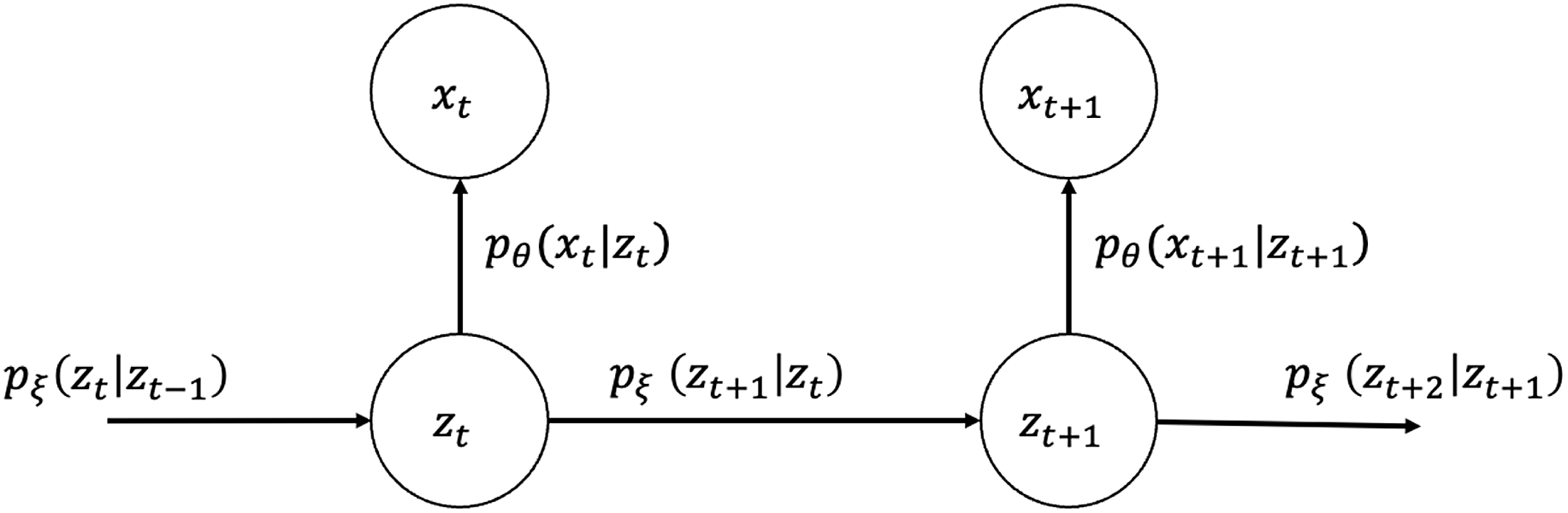
Figure 1. Graphical model representation of state-space LC.
Although a drifted RW is assumed for
 $ {p}_{\xi }\!\left({z}_{t+1}|{z}_{t}\right)$
as in the original LC model, we propose a generalization by replacing
$ {p}_{\xi }\!\left({z}_{t+1}|{z}_{t}\right)$
as in the original LC model, we propose a generalization by replacing
 $ \alpha +{\kappa }_{t}\beta $
in Equation (2.4) with a nonlinear vector-valued function denoted by
$ \alpha +{\kappa }_{t}\beta $
in Equation (2.4) with a nonlinear vector-valued function denoted by
 $ {f}_{\theta }\!\left({z}_{t}\right),$
where the function belongs to a broad nonlinear function class that can be obtained by a NN.
$ {f}_{\theta }\!\left({z}_{t}\right),$
where the function belongs to a broad nonlinear function class that can be obtained by a NN.
Using
 $ {x}_{t}=\mathrm{log}\;{m}_{t}=\left({\mathrm{log}\;m}_{t,0},\mathrm{log}\;{m}_{t,1},\dots ,\mathrm{log}\;{m}_{t,n}\right),$
our model is given by:
$ {x}_{t}=\mathrm{log}\;{m}_{t}=\left({\mathrm{log}\;m}_{t,0},\mathrm{log}\;{m}_{t,1},\dots ,\mathrm{log}\;{m}_{t,n}\right),$
our model is given by:
 \begin{equation}\begin{split}\mathrm{log}\;{m}_{t}={f}_{\theta }\!\left({z}_{}\right)+{\varepsilon }_{t},\\[5pt]{z}_{t}\text{ = }{\mu }_{\xi }+{z}_{t-1}+{\sigma }_{\xi }{\eta }_{t}, t > 1\\[5pt]{z}_{1}\text{ = }{z}_{0}+{\sigma }_{\xi }{\eta }_{1}\end{split}\end{equation}
where
 $ {\varepsilon }_{t}$
and
$ {\varepsilon }_{t}$
and
 $ {\eta }_{t}$
are
$ {\eta }_{t}$
are
 $ iid$
noises that
$ iid$
noises that
 $ {\varepsilon }_{t}\;~\;N\!\left(0,{\sum }_{\theta }\right)\!;\;{\sum }_{\theta }=diag({{\sigma }_{\theta }}_{0}^{2}, {{\sigma }_{\theta }}_{1}^{2},\dots ,$
 $ {{\sigma }_{\theta }}_{n}^{2});\;{\eta }_{t}\;~\;N(\mathrm{0,1})$
.
$ {{\sigma }_{\theta }}_{n}^{2});\;{\eta }_{t}\;~\;N(\mathrm{0,1})$
.
Note that
 $ \left({{\sigma }_{\theta }}_{0}^{2},{{\sigma }_{\theta }}_{1}^{2},\dots ,{{\sigma }_{\theta }}_{n}^{2}\right)$
, (
$ \left({{\sigma }_{\theta }}_{0}^{2},{{\sigma }_{\theta }}_{1}^{2},\dots ,{{\sigma }_{\theta }}_{n}^{2}\right)$
, (
 $ {\mu }_{\xi }$
,
$ {\mu }_{\xi }$
,
 $ {\sigma }_{\xi }$
) and the initial value
$ {\sigma }_{\xi }$
) and the initial value
 $ {z}_{0}$
can be obtained as learning parameters of a NN.
$ {z}_{0}$
can be obtained as learning parameters of a NN.
Assuming that
 $ {p}_{\xi }\!\left({z}_{1}\right)$
follows a normal distribution, the log-likelihood of the generative distribution to be maximized is given as follows:
$ {p}_{\xi }\!\left({z}_{1}\right)$
follows a normal distribution, the log-likelihood of the generative distribution to be maximized is given as follows:
 \begin{equation}\mathrm{log}\;{p}_{\theta }\!\left({x}_{t}|{z}_{t}\right)=-\mathrm{log}\sqrt{{\left(2\pi \right)}^{n+1}\left|{\sum }_{\theta }\right|}-\frac{1}{2}{\left({x}_{t}-{f}_{\theta }\!\left({z}_{t}\right)\right)}^{\mathrm{T}}{{\sum }_{\theta }}^{-1}\!\left({x}_{t}-{f}_{\theta }\!\left({z}_{t}\right)\right),\end{equation}
where
 $ \left|{\sum }_{\theta }\right|={{\sigma }_{\theta }}_{0}^{2}{{\sigma }_{\theta }}_{1}^{2}\dots {{\sigma }_{\theta }}_{n}^{2}$
.
$ \left|{\sum }_{\theta }\right|={{\sigma }_{\theta }}_{0}^{2}{{\sigma }_{\theta }}_{1}^{2}\dots {{\sigma }_{\theta }}_{n}^{2}$
.
5. VAE for the model
In this section, a VAE is used to estimate the parameters of the state-space model, and the state-space model specification chosen will determine the expression for the loss function used when fitting the VAE to data.
5.1. The loss function
To apply the GDM for the variational inference, it is necessary to derive the loss function given by the sign-reversed ELBO of the model. The joint posterior distribution
 $ {p}_{\theta }({z}_{1},{z}_{2},\dots ,{z}_{T}|{x}_{1},{x}_{2},\dots ,{x}_{T})$
with the generative parameter
$ {p}_{\theta }({z}_{1},{z}_{2},\dots ,{z}_{T}|{x}_{1},{x}_{2},\dots ,{x}_{T})$
with the generative parameter
 $ \theta $
is approximated by
$ \theta $
is approximated by
 $ {q}_{\varphi }\!\left({z}_{1},{z}_{2},\dots ,{z}_{T}|{x}_{1},{x}_{2},\dots ,{x}_{T}\right)$
with variational parameter
$ {q}_{\varphi }\!\left({z}_{1},{z}_{2},\dots ,{z}_{T}|{x}_{1},{x}_{2},\dots ,{x}_{T}\right)$
with variational parameter
 $ \varphi $
where the approximation distribution
$ \varphi $
where the approximation distribution
 $ {q}_{\varphi }$
is assumed to be factorizable as expressed in Equation (3.1). The structure of the VAE used for the variational inference of the proposed model is represented in a graphical model (Figure 2) where the vertical network at each time
$ {q}_{\varphi }$
is assumed to be factorizable as expressed in Equation (3.1). The structure of the VAE used for the variational inference of the proposed model is represented in a graphical model (Figure 2) where the vertical network at each time
 $ t$
has an AE structure with encoder
$ t$
has an AE structure with encoder
 $ {q}_{\varphi }\!\left({z}_{t}|{x}_{t}\right)$
and decoder
$ {q}_{\varphi }\!\left({z}_{t}|{x}_{t}\right)$
and decoder
 $ {p}_{\theta }\!\left({x}_{t}\right|{z}_{t})$
.
$ {p}_{\theta }\!\left({x}_{t}\right|{z}_{t})$
.
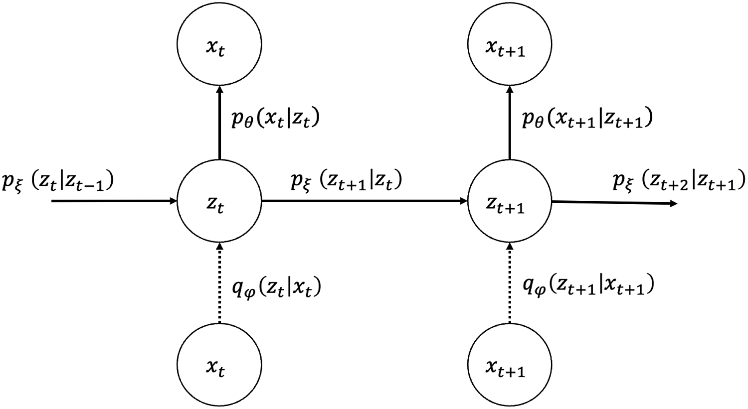
Figure 2. Graphical model representation of VAE for state-space LC (dotted line: approximation).
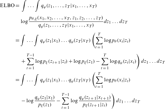
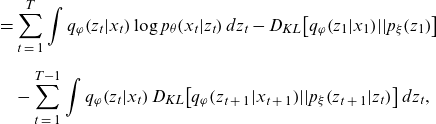
The ELBO to be maximized for the proposed model is given by:
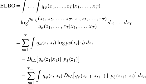 \begin{align}\mathrm{E}\mathrm{L}\mathrm{B}\mathrm{O}\mathrm{}\mathrm{} & =\int \dots \int {q}_{\varphi }\!\left({z}_{1},\dots ,{z}_{T}|{x}_{1},\dots ,{x}_{T}\right)\nonumber\\[5pt] &\quad \mathrm{log}\frac{{p}_{\theta ,\;\xi }\!\left({x}_{1},{x}_{2},\dots ,{x}_{T},{z}_{1},{z}_{2},\dots ,{z}_{T}\right)}{{q}_{\varphi }\!\left({z}_{1},\dots ,{z}_{T}|{x}_{1},\dots ,{x}_{T}\right)}d{z}_{1}\dots d{z}_{T}\nonumber\\[5pt]&=\sum _{t=1}^{T}\int {q}_{\varphi }\!\left({z}_{t}|{x}_{t}\right)\mathrm{log}\;{p}_{\theta }\!\left({x}_{t}|{z}_{t}\right)d{z}_{t}\nonumber\\[5pt]&\quad -{D}_{kL}\!\left[{q}_{\varphi }\!\left({z}_{1}|{x}_{1}\right)\!\left|\right|{p}_{\xi }\!\left({z}_{1}\right)\right]\nonumber\\[5pt]&\quad-\sum _{t=1}^{T-1}\int {q}_{\varphi }\!\left({z}_{t}|{x}_{t}\right){D}_{kL}\!\left[{q}_{\varphi }\!\left({z}_{t+1}|{x}_{t+1}\right)\left|\right|{p}_{\xi }\!\left({z}_{t+1}|{z}_{t}\right)\right]d{z}_{t},\end{align}
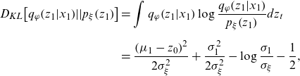
where the KL terms can be calculated analytically from the assumptions, given by Equation (3.6) and (4.2), as follows:
 \begin{equation*}{D_{KL}}\!\left[ {{q_\varphi }\!\left( {{z_1}|{x_1}} \right)\!||{p_\xi }\!\left( {{z_1}} \right)} \right] = \frac{{{{\left( {{\mu _1} - {z_0}} \right)}^2}}}{{2\sigma _\xi ^2}} + \frac{{\sigma _1^2}}{{2\sigma _\xi ^2}} - \log \frac{{{\sigma _1}}}{{{\sigma _\xi }}} - \frac{1}{2},\end{equation*}
 \begin{align*}{D_{KL}}\!\left[ {{q_\varphi }\!\left( {{z_{t\;+\;1}}|{x_{t\;+\;1}}} \right)||{p_\xi }\!\left( {{z_{t\;+\;1}}|{z_t}} \right)} \right] &= \frac{{{{\left( {{\mu _{t\;+\;1}} - \left( {{\mu _\xi } + {z_t}} \right)} \right)}^2}}}{{2\sigma _\xi ^2}} + \frac{{\sigma _{t\;+\;1}^2}}{{2\sigma _\xi ^2}} - \log \frac{{{\sigma _t}}}{{{\sigma _\xi }}} \\[5pt] & \quad - \frac{1}{2},\;t \ge 1.\;\end{align*}
Replacing
 ${z_t}\;$
in Equation (5.1) with the sampling approximations {
${z_t}\;$
in Equation (5.1) with the sampling approximations {
 ${z_{l,t}}$
} that follows the reparametrized distribution
${z_{l,t}}$
} that follows the reparametrized distribution
 $g_{\varphi}(x_{t},\epsilon_{t})$
given by Equation (3.6), the ELBO is approximated by:
$g_{\varphi}(x_{t},\epsilon_{t})$
given by Equation (3.6), the ELBO is approximated by:
 \begin{align}{\rm{ELBO}} &\approx \frac{1}{L}\mathop \sum \limits_{l\;=\;1}^L \left( \mathop \sum \limits_{t\;=\;1}^T \log {p_\theta }\!\left( {{x_t}|{z_{l,t}}} \right) - {D_{kL}}\!\left[ {{q_\varphi }\!\left( {{z_1}|{x_1}} \right)||{p_\xi }\!\left( {{z_1}} \right)} \right] \right. \nonumber\\[5pt]& \quad \left. - \mathop \sum \limits_{t\;=\;1}^{T - 1} {D_{KL}}\!\left[ {{q_\varphi }\!\left( {{z_{l,t\;+\;1}}|{x_{t\;+\;1}}} \right)\!||{p_\xi }\!\left( {{z_{l,t\;+\;1}}|{z_{l,t}}} \right)} \right] \right).\end{align}
Finally, the loss function (i.e., sign-reversed ELBO) is given by:
 \begin{equation} - \frac{1}{L}\mathop \sum \limits_{l\;=\;1}^L \left( {\mathop \sum \limits_{t\;=\;1}^T \left( {\log {p_\theta }\!\left( {{x_t}|{z_{l,t}}} \right) - \frac{{{{\left( {{\mu _t} - \left( {{\mu _\xi } + {z_{l,t - 1}}} \right)} \right)}^2}}}{{2\sigma _\xi ^2}} - \frac{{\sigma _t^2}}{{2\sigma _\xi ^2}} + \log \frac{{{\sigma _t}}}{{{\sigma _\xi }}} + \frac{1}{2}} \right)} \right),\end{equation}
where
 ${z_{l,0}} = {z_0} - {\mu _\xi }$
, and
${z_{l,0}} = {z_0} - {\mu _\xi }$
, and
 $\log {p_\theta }\!\left( {{x_t}|{z_{l,t}}} \right)$
is obtained by replacing
$\log {p_\theta }\!\left( {{x_t}|{z_{l,t}}} \right)$
is obtained by replacing
 ${z_t}\;$
in Equation (4.3) with
${z_t}\;$
in Equation (4.3) with
 ${z_{l,t}}$
. Note that
${z_{l,t}}$
. Note that
 $\left( {{\sigma _\theta }_0^2,{\sigma _\theta }_1^2, \ldots ,{\sigma _\theta }_n^2} \right)$
, (
$\left( {{\sigma _\theta }_0^2,{\sigma _\theta }_1^2, \ldots ,{\sigma _\theta }_n^2} \right)$
, (
 ${\mu _\xi }$
,
${\mu _\xi }$
,
 ${\sigma _\xi }$
),
${\sigma _\xi }$
),
 $\;{z_0}\;$
and
$\;{z_0}\;$
and
 $\left( {{\mu _t},{\sigma _t}} \right)$
given by Equation (3.6) are learning parameters in the VAE network. Details of the derivation of the loss function are given in Appendix.
$\left( {{\mu _t},{\sigma _t}} \right)$
given by Equation (3.6) are learning parameters in the VAE network. Details of the derivation of the loss function are given in Appendix.
The mortality predictions can be obtained by decoding the projected state random variable
 ${z_{t,}}\;$
in the form of mean values or confidence intervals.
${z_{t,}}\;$
in the form of mean values or confidence intervals.
5.2. The network configuration
The proposed VAE has an FCN architecture comprising three hidden layers between the input and output layers; it has the following specifications:
-
Although the numbers of neurons in the first and third hidden layers are variable, the number of neurons in the latent layer (second hidden layer) is fixed at 1 to be consistent with the dimension of the state random variable
${z_t}.$
-
Both the encoder and decoder use hyperbolic tangent sigmoidal function and identity function as activation functions.
-
The encoder (first hidden layer) includes the reparameterization unit given in Equation (3.6).
-
A fixed age-impact vector corresponding to
$\alpha $
in Equation (2.4) is used as a learning parameter that is deducted before encoding and added after decoding, whose initial value is given by a vector of the age-specific averages of the observed log-mortality rates.


The architecture is illustrated in Figure 3. The model is coded from scratch in Python without using optimization packages, and the codes for the most characteristic part of the model are presented in the online Supplementary Material.
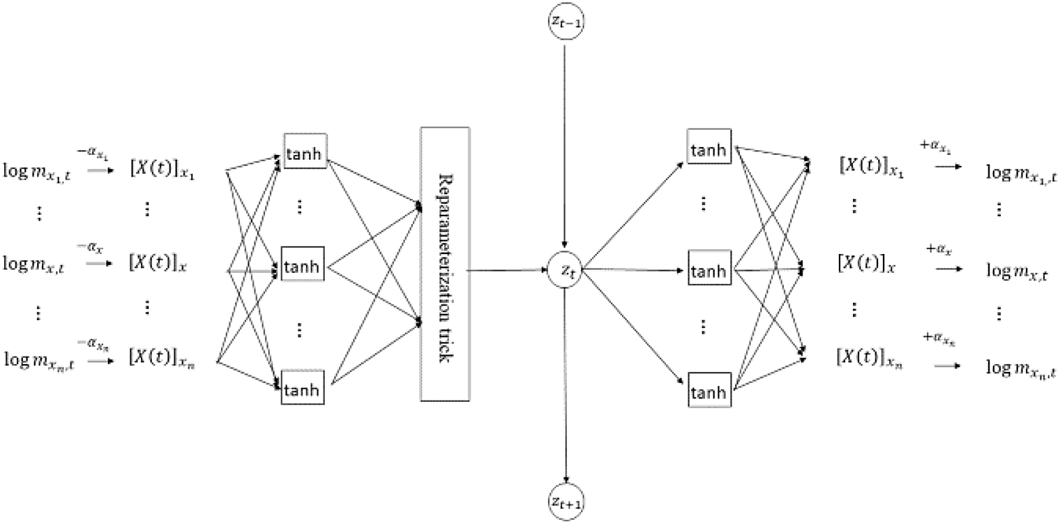
Figure 3. Network architecture of VAE.
6. Numerical application
This section shows the results of applying the proposed model to the data from the HMD. The HMD data used here are the central mortality rates for ages 0–99 years, mixed gender, from 1961 to 2018. In this study, the observation period begins in 1961 to coincide with the introduction of the universal health insurance in Japan. For the accuracy evaluation, the data are divided into training data from 1961 to 2000 and test data from 2001 to 2018.
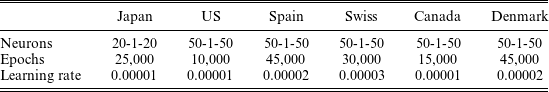
6.1. Calibration procedures
The hyperparameters to be determined for our model are the learning rate, the number of learning epochs, and the number of neurons in the first and third hidden layers. The number of neurons in the second hidden layer is fixed at 1 to be consistent with the dimension of the state variable of the model. The hyperparameters are selected to minimize the median of 10 minimum squared errors (MSEs), which correspond to 10 random seeds, over the validation data that consist of the latter 5 years (i.e., from 1996 to 2000) of the original training data; the selection universe of the hyperparameters contains the numbers of epochs from 5000 to 50,000 and the numbers of neurons in the three hidden layers from 10–1–10 to 50–1–50, where the configurations are limited to the symmetric type (i.e., the same number of neurons in the first and third hidden layers) common in AEs. Note that cross-validations are not available for time series models including our model. Since a larger number of epochs reduces the effect of the number of samples for the Monte Carlo integration of the loss function, the number L in Equation (5.3) is fixed at 10. The validated hyperparameters for six countries, including Japan and the United States (US), are given as follows.
The model, which is coded from scratch in Python without using optimization packages, requires a relatively large number of epochs as shown in Table 1, but the total run-time per country is about 10 min in the Google Colaboratory (https://colab.research.google.com) due to its shallow network structure. Although not used in this study, normalizing the input data to being centered with unit variance can reduce the number of epochs.
Table 1 Validated hyperparameters for six countries.
6.2. Performance comparison with LC
Using the hyperparameters given in Table 1, prediction performances are estimated in the same way over the test data. Table 2 summarizes the comparison of the prediction accuracy between LC (SVD+RW) and the VAE over the test data for six countries, where the accuracy measure is the same MSE as for the validation of the hyperparameters.
Table 2 MSE comparison between VAE and LC over test data for six countries.
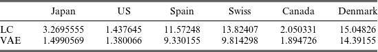
The observation period for the training data begins in 1961, when the universal health insurance was introduced in Japan, but longer observation periods are likely to improve forecasting accuracy in other countries. This model fits both in the context of the literature on BSS mortality models, where prediction accuracy is not often discussed, and in the context of the literature on NN models for mortality prediction, where prediction accuracy is the focus. As a NN model, this model focuses more on achieving features not found in previous NN models than on prediction accuracy, as shown in the following sections. In the following sections, we will focus our analysis on Japan and US.
6.3. Interpretability of the model
In this section, the interpretability, one of the key features of the model, is demonstrated by the comparison of the components of the model with all parameters of LC over the training data for Japan and US, using the hyperparameters given in Table 1.
Figure 4 gives the comparison of LC’s year-specific factor
 ${\kappa _t}\;$
with
${\kappa _t}\;$
with
 ${\mu _t}$
, denoting the mean of the latent factor of the VAE generated by one random seed, over the training data for Japan and US. The descending curves of
${\mu _t}$
, denoting the mean of the latent factor of the VAE generated by one random seed, over the training data for Japan and US. The descending curves of
 ${\mu _t}\;$
can be interpreted as indicating medical progress as well as the LC’s year-specific factor
${\mu _t}\;$
can be interpreted as indicating medical progress as well as the LC’s year-specific factor
 ${\kappa _t}$
. The slope of
${\kappa _t}$
. The slope of
 ${\rm{\;}}{\mu _t}$
is more gradual than that of
${\rm{\;}}{\mu _t}$
is more gradual than that of
 ${\kappa _t}$
, for both Japan and US, indicating that excessive mortality reductions in the long-term predictions are less likely to occur than in LC.
${\kappa _t}$
, for both Japan and US, indicating that excessive mortality reductions in the long-term predictions are less likely to occur than in LC.

Figure 4. VAE’s
 ${\mu _t}$
and LC’s
${\mu _t}$
and LC’s
 ${\kappa _t}\;$
over training data for Japan (left) and US (right).
${\kappa _t}\;$
over training data for Japan (left) and US (right).
Figure 5 compares LC’s age sensitivity factor
 $\beta \;$
and the decoder’s sensitivity to
$\beta \;$
and the decoder’s sensitivity to
 ${\mu _t},$
given by
${\mu _t},$
given by
 $\;\frac{d}{{d{\mu _t}}}{f_\theta }\!\left( {{\mu _t}} \right)$
for one random seed, for all ages in 1970, 1980, 1990, and 2000, over the training data for Japan and US. The number of humps in the decoder’s sensitivity curves is roughly similar to that of LC’s age sensitivity factor
$\;\frac{d}{{d{\mu _t}}}{f_\theta }\!\left( {{\mu _t}} \right)$
for one random seed, for all ages in 1970, 1980, 1990, and 2000, over the training data for Japan and US. The number of humps in the decoder’s sensitivity curves is roughly similar to that of LC’s age sensitivity factor
 $\beta $
, for both Japan and US, capturing country-specific characteristics.
$\beta $
, for both Japan and US, capturing country-specific characteristics.
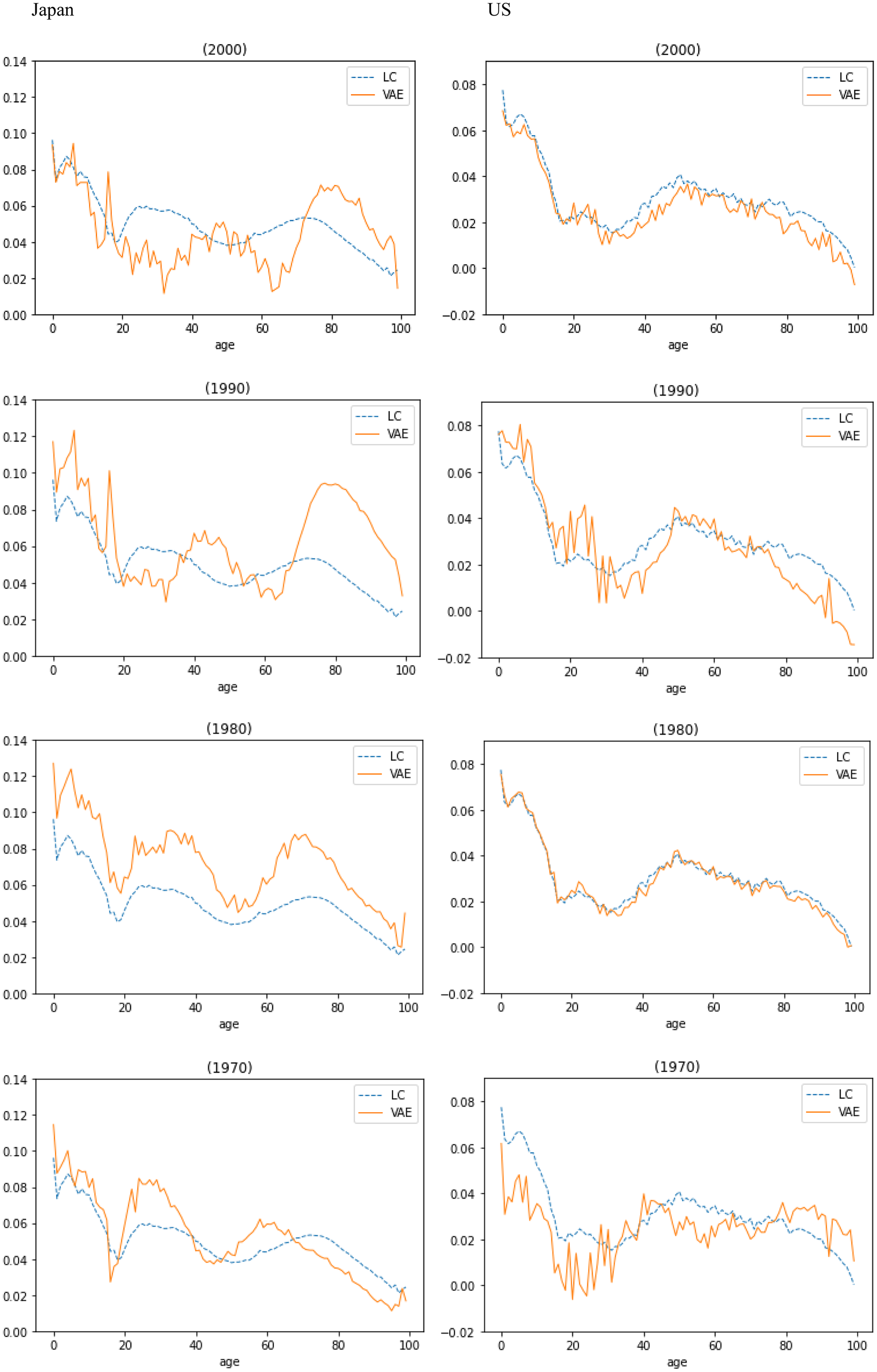
Figure 5. Decoder’s sensitivity to
 ${\mu _{t\;}}$
and LC’s
${\mu _{t\;}}$
and LC’s
 $\beta \;$
over training data for Japan (left) and US (right).
$\beta \;$
over training data for Japan (left) and US (right).
Figure 6 shows that the learning parameter
 $\alpha $
of the VAE, generated by one random seed, is consistent with the fixed age factor
$\alpha $
of the VAE, generated by one random seed, is consistent with the fixed age factor
 $\alpha $
of LC, given by the averaged mortality, over the training data for Japan and US.
$\alpha $
of LC, given by the averaged mortality, over the training data for Japan and US.
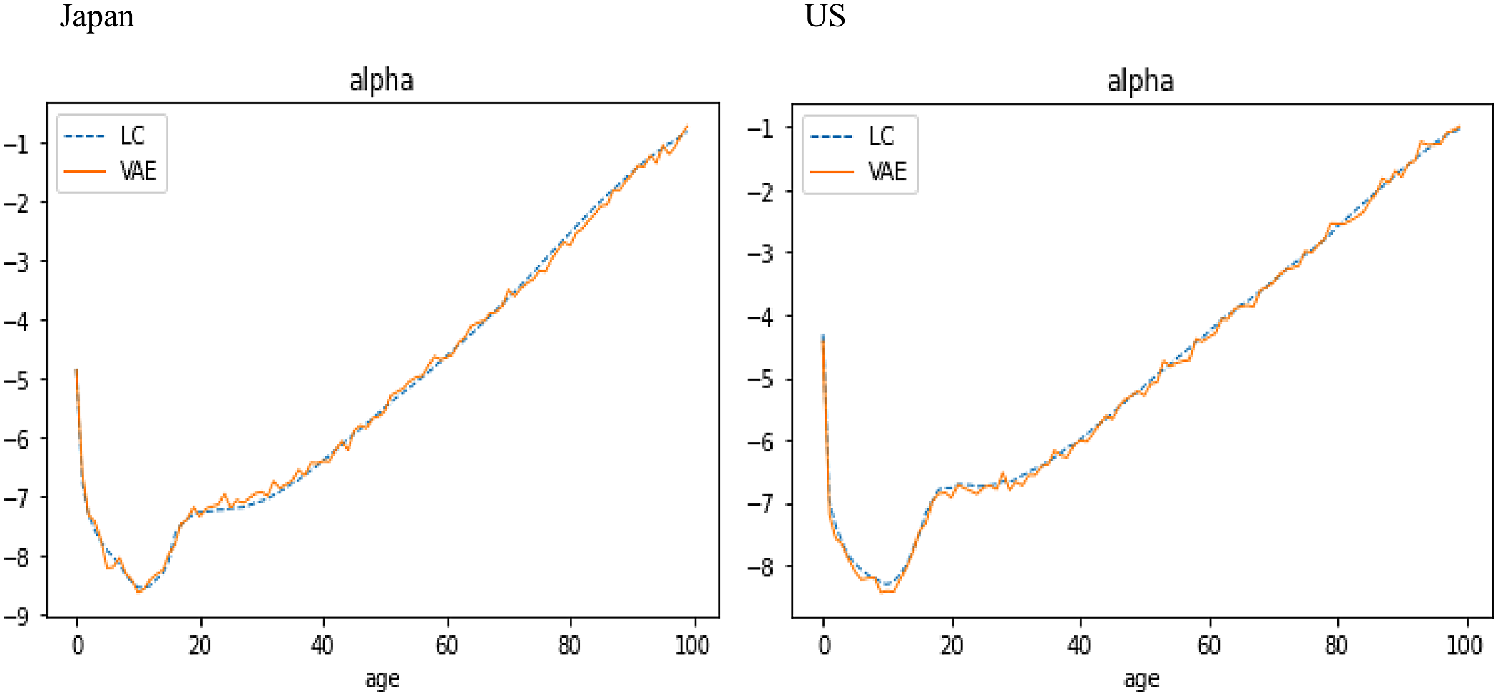
Figure 6. VAE’s
 $\alpha $
and LC’s
$\alpha $
and LC’s
 $\alpha \;$
over training data for Japan (left) and US (right).
$\alpha \;$
over training data for Japan (left) and US (right).
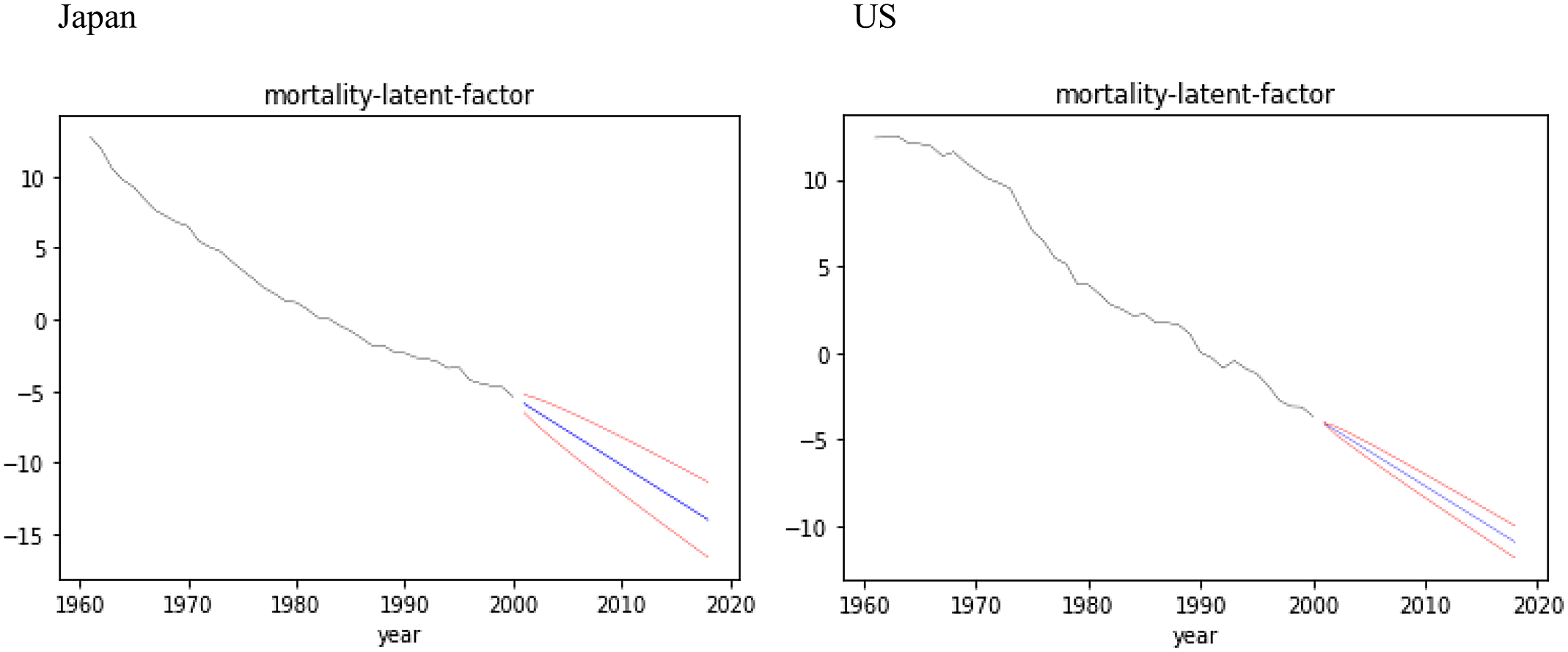
Figure 7. Forecasts with confidence intervals for latent factor
 ${\rm{\;}}{z_t}$
over test data for Japan (left) and US (right).
${\rm{\;}}{z_t}$
over test data for Japan (left) and US (right).
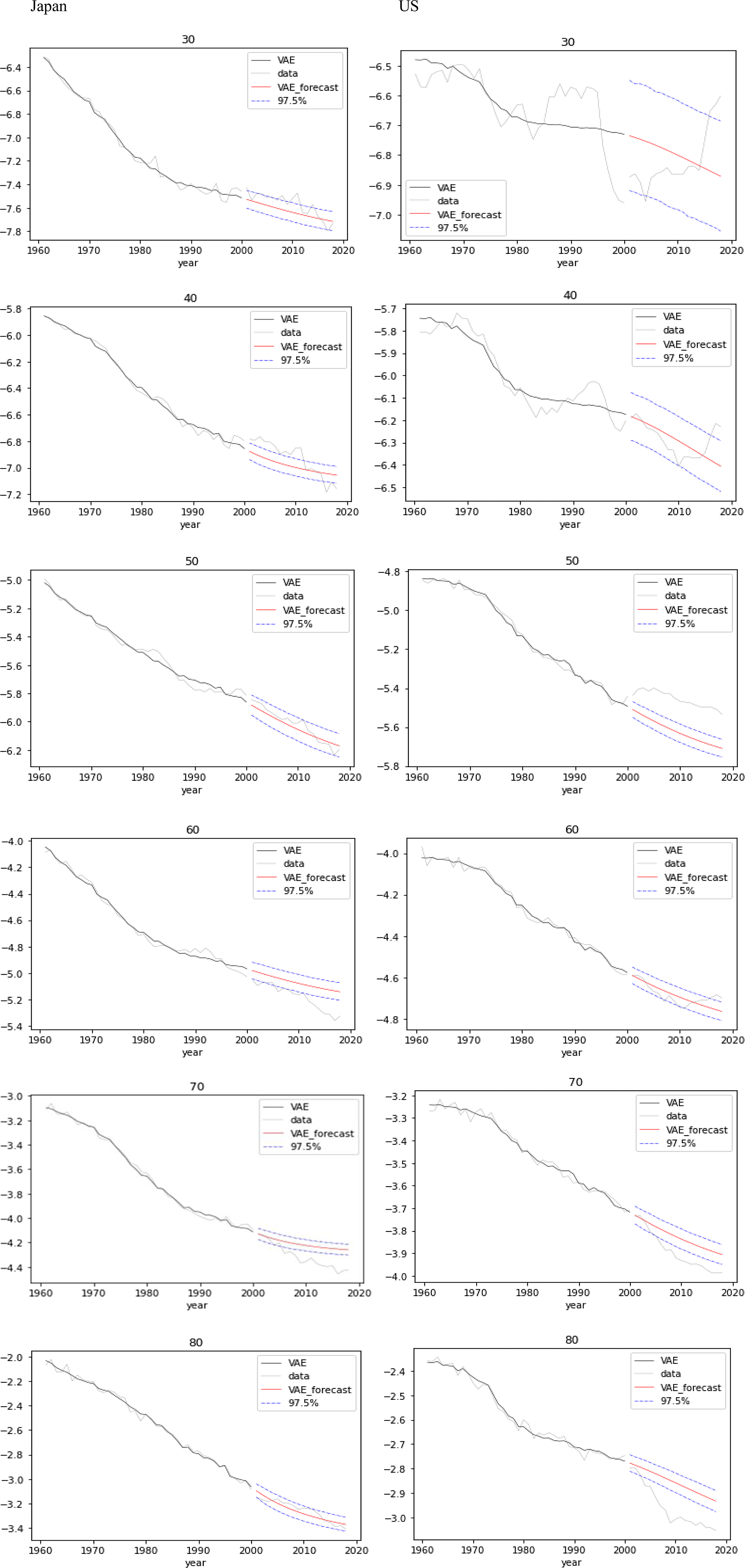
Figure 8. Forecasts with confidence intervals for mortality by age (from 30 to 80 years) over test data for Japan (left) and US (right).
6.4. Forecasts with confidence intervals
Existing NN models for the mortality forecasts with confidence intervals are solely based on the exogenously given randomness such as random seed for NNs or added randomness for the time series models in two-stage estimations. In this section, we show that our model has an ability to forecast mortality with confidence intervals based on the endogenous randomness, as with BSS formulations, using the hyperparameters given in Table 1.
Figure 7 shows the forecasts with 97.5% confidence intervals for the latent factor
 ${z_t}\;$
over the test data for Japan and US, appending
${z_t}\;$
over the test data for Japan and US, appending
 ${\mu _t}\;$
over the training data. The natural connection between the mean
${\mu _t}\;$
over the training data. The natural connection between the mean
 ${\mu _t}$
of the latent variable encoded over the training data and the mean of the state model
${\mu _t}$
of the latent variable encoded over the training data and the mean of the state model
 ${z_t}\;$
estimated over the test data shows the effect of the variational approximation.
${z_t}\;$
estimated over the test data shows the effect of the variational approximation.
Figure 8 gives mortality forecasts with 97.5% confidence intervals at ages 30, 40, 50, 60, 70, and 80 years over the test data for Japan and US, appending the actual mortality and the reconstructed mortality over the training data.
6.5. Remarks on changing number of neurons
The prediction accuracy of the VAE model is generally improved by increasing the number of neurons in the first and third hidden layers. Table 3 summarizes the comparison of the prediction accuracy by MSE of LC and VAE models (from 10–1–10 to 50–1–50) over the test data for Japan and US, using a fixed number of epochs per country. The results demonstrate that the number of neurons in a VAE that can outperform LC varies among countries and that if the number of neurons is extremely large, the prediction accuracy decreases because of overlearning.
We also consider the smoothness of mortality curves in ultralong-term predictions desirable in the economic valuation of insurance/pension liabilities and longevity risk management.
Figure 9 shows the 50-year predictions of Japanese mortality by VAE (from 10–1–10 to 50–1–50), where the dark-colored curves are the predictions. For the 50-year projection in Japan, all data (i.e., from 1961 to 2018) are used for the training data.
Table 3 MSE comparison of LC and VAE (from 10-1-10 to 50-1-50) over test data for Japan and US.
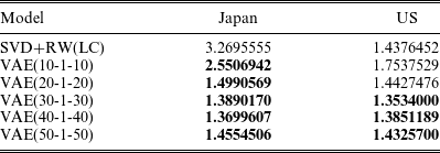
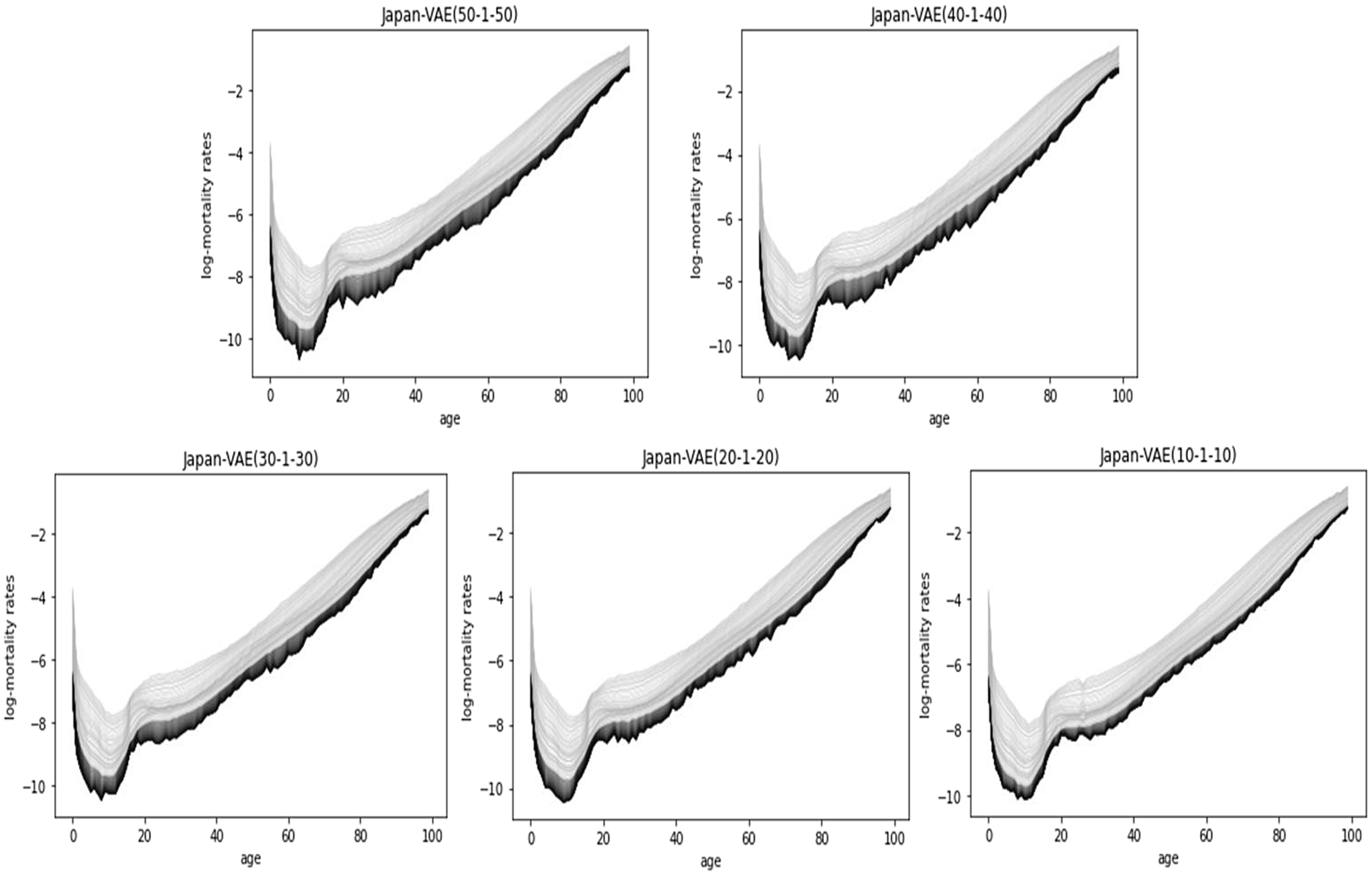
Figure 9. Fifty-year predictions by VAE (from 10–1–10 to 50–1–50), Japan.
Improving the prediction accuracy of VAE trades-off with the smoothness of the prediction curves, but introducing an asymmetric configuration into the hidden layers of VAE can improve the smoothness of prediction while maintaining high prediction accuracy. It is effective to increase and decrease the numbers of neurons in the first and third hidden layers, respectively.
For example, VAE (50–1–3) yields relatively smooth prediction curves as shown in Figure 10, and the prediction accuracy (MSE:3.0416) remains better than LC (MSE:3.2696) on the same data as for Table 3.

Figure 10. Fifty-year prediction by VAE(50-1-3), Japan.
7. Conclusions
This paper proposes a NN-based generalization of LC using VAE that performs mortality forecasts with confidence intervals based on the endogenous randomness (i.e., not by seed randomness for NNs), as with the BSS models, in a single-stage procedure without losing interpretability of the model. Our model fills a gap in the literature of NN extensions of LC, since previous NN models either enable single-step estimation of parameters but lose interpretability of the model, or retain interpretability but estimate parameters in two steps. The model also can yield relatively smooth mortality curves in long-term predictions due to the dimensionality reduction capability of the VAE.
However, our model has the limitations that it employs a 1D RW with
 $iid$
residuals for the latent state model, and thus the number of neurons in the second hidden layer is limited to one; the limitations are intended to avoid sampling approximations of multiple integrals that reduce estimation efficiency and often require MCMC. Dimensional extensions of the latent state model (i.e., multiple neurons in the second hidden layer) and the introduction of the non-
$iid$
residuals for the latent state model, and thus the number of neurons in the second hidden layer is limited to one; the limitations are intended to avoid sampling approximations of multiple integrals that reduce estimation efficiency and often require MCMC. Dimensional extensions of the latent state model (i.e., multiple neurons in the second hidden layer) and the introduction of the non-
 $iid$
residuals to the latent state model are future work; they can improve representation capabilities of the model and may allow its extension to cohort and multiple population models. However, if one has multiple neurons in the second hidden layer and may have to deal with an identifiability issue, see Example 7.28 in Wüthrich and Merz (Reference Wüthrich and MERZ2022).
$iid$
residuals to the latent state model are future work; they can improve representation capabilities of the model and may allow its extension to cohort and multiple population models. However, if one has multiple neurons in the second hidden layer and may have to deal with an identifiability issue, see Example 7.28 in Wüthrich and Merz (Reference Wüthrich and MERZ2022).
Acknowledgments
The authors thank the anonymous referees for valuable comments which helped to improve the paper substantially.
Supplementary material
To view supplementary material for this article, please visit http://doi.org/10.1017/asb.2022.15.
Appendix
Derivation of the loss function
The joint distribution
 ${p_{\theta ,\;\xi }}\!\left( {{x_1},{x_2}, \ldots ,{x_T},{z_1},{z_2}, \ldots ,{z_T}} \right)$
following Equation (4.2) satisfies
${p_{\theta ,\;\xi }}\!\left( {{x_1},{x_2}, \ldots ,{x_T},{z_1},{z_2}, \ldots ,{z_T}} \right)$
following Equation (4.2) satisfies
 \begin{align*}\log {p_{\theta ,\xi }}\!\left( {{x_1},{x_2}, \ldots ,{x_T},{z_1},{z_2}, \ldots ,{z_T}} \right) & = \mathop \sum \limits_{t\;=\;1}^T \log {p_\theta }\!\left( {{x_t}|{z_t}} \right) \\[5pt] & \quad + \mathop \sum \limits_{t\;=\;1}^{T - 1} \log {p_\xi }\!\left( {{z_{t\;+\;1}}|{z_t}} \right) + \log {p_\xi }\!\left( {{z_1}} \right).\end{align*}
Using the above equation and the mean field approximation given by Equation (3.1), the ELBO of the model can be rewritten as follows:
 \begin{align*}{\rm{ELBO}} & = \;\int \ldots \int {q_\varphi }\!\left( {{z_1}, \ldots ,{z_T}|{x_1}, \ldots ,{x_T}} \right) \nonumber \\[5pt] & \quad \log \frac{{{p_{\theta ,\xi }}\!\left( {{x_1},{x_2}, \ldots ,{x_T},{z_1},{z_2}, \ldots ,{z_T}} \right)}}{{{q_\varphi }\!\left( {{z_1}, \ldots ,{z_T}|{x_1}, \ldots ,{x_T}} \right)}}d{z_1} \ldots d{z_T}\nonumber \\[5pt] &= \int \ldots \int {q_\varphi }\!\left( {{z_1}|{x_1}} \right) \ldots {q_\varphi }\!\left( {{z_T}|{x_T}} \right)\left( \mathop \sum \limits_{t\;=\;1}^T \log {p_\theta }\!\left( {{x_t}|{z_t}} \right) \right. \nonumber \\[5pt] & \left. \quad + \mathop \sum \limits_{t\;=\;1}^{T - 1} \log {p_\xi }\!\left( {{z_{t\;+\;1}}|{z_t}} \right) + \log {p_\xi }\!\left( {{z_1}} \right) - \mathop \sum \limits_{t\;=\;1}^T \log {q_\varphi }\!\left( {{z_t}|{x_t}} \right) \right)d{z_1} \ldots d{z_T}\nonumber \\ & = \int \ldots \int {q_\varphi }\!\left( {{z_1}|{x_1}} \right) \ldots {q_\varphi }\!\left( {{z_T}|{x_T}} \right)\left( \mathop \sum \limits_{t\;=\;1}^T \log {p_\theta }\!\left( {{x_t}|{z_t}} \right) \right.\nonumber \\[5pt] & \left. \quad - \log \frac{{{q_\varphi }\!\left( {{z_1}|{x_1}} \right)}}{{{p_\xi }\!\left( {{z_1}} \right)}} - \mathop \sum \limits_{t\;=\;1}^{T - 1} \log \frac{{{q_\varphi }\!\left( {{z_{t\;+\;1}}|{x_{t\;+\;1}}} \right)}}{{{p_\xi }\!\left( {{z_{t\;+\;1}}|{z_t}} \right)}} \right)d{z_1} \ldots d{z_T} \end{align*}
 \begin{align} &= \mathop \sum \limits_{t\;=\;1}^T \int {q_\varphi }\!\left( {{z_t}|{x_t}} \right)\log {p_\theta }\!\left( {{x_t}|{z_t}} \right)d{z_t} - {D_{KL}}\!\left[ {{q_\varphi }\!\left( {{z_1}|{x_1}} \right)\!||{p_\xi }\!\left( {{z_1}} \right)} \right] \nonumber \\[5pt] & \quad - \mathop \sum \limits_{t\;=\;1}^{T - 1} \int {q_\varphi }\!\left( {{z_t}|{x_t}} \right){D_{KL}}\!\left[ {{q_\varphi }\!\left( {{z_{t\;+\;1}}|{x_{t\;+\;1}}} \right)\!||{p_\xi }\!\left( {{z_{t\;+\;1}}|{z_t}} \right)} \right]d{z_t},\end{align}
where, from the assumptions given by Equation (3.6) and (4.2), the components of the KL terms follow the normal distributions as follows:
 \begin{equation*}{q_\varphi }\!\left( {{z_1}|{x_1}} \right) = \frac{1}{{\sqrt {2\pi } {\sigma _1}}}{e^{ - \;\frac{{{{\left( {{z_1} - {\mu _1}} \right)}^2}}}{{2{\sigma _1}^2}}}},\end{equation*}
 \begin{equation*}{p_\xi }\!\left( {{z_1}} \right) = \frac{1}{{\sqrt {2\pi } {\sigma _\xi }}}{e^{ - \;\frac{{{{\left( {{z_1} - {z_0}} \right)}^2}}}{{2\sigma _\xi ^2}}}},\end{equation*}
 \begin{equation*}{q_\varphi }\!\left( {{z_{t\;+\;1}}|{x_{t\;+\;1}}} \right) = \frac{1}{{\sqrt[{}]{{2\pi }}{\sigma _{t\;+\;1}}}}{e^{ - \;\frac{{{{\left( {{z_{t\;+\;1}} - {\mu _{t\;+\;1}}} \right)}^2}}}{{2{\sigma _{t\;+\;1}}^2}}}},\end{equation*}
 \begin{equation*}{p_\xi }\!\left( {{z_{t\;+\;1}}{\rm{|}}{z_t}} \right) = \frac{1}{{\sqrt[{}]{{2\pi }}{\sigma _\xi }}}{e^{ - \;\frac{{{{\left( {{z_{t\;+\;1}} - \left( {{\mu _\xi } + {z_t}} \right)} \right)}^2}}}{{2{\sigma _\xi }^2}}}},\;\;t \ge 1.\end{equation*}
Then the KL terms in Equation (A1) can be calculated analytically as follows:
 \begin{align} {D_{KL}}\!\left[ {{q_\varphi }\!\left( {{z_1}|{x_1}} \right)\!||{p_\xi }\!\left( {{z_1}} \right)} \right] & = \int {q_\varphi }\!\left( {{z_1}|{x_1}} \right)\log \frac{{{q_\varphi }\!\left( {{z_1}|{x_1}} \right)}}{{{p_\xi }\!\left( {{z_1}} \right)}}d{z_t}\nonumber \\[5pt] & = \frac{{{{\left( {{\mu _1} - {z_0}} \right)}^2}}}{{2\sigma _\xi ^2}} + \frac{{\sigma _1^2}}{{2\sigma _\xi ^2}} - \log \frac{{{\sigma _1}}}{{{\sigma _\xi }}} - \frac{1}{2}, \end{align}
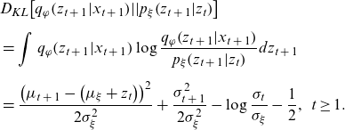 \begin{align} & {D_{KL}}\!\left[ {{q_\varphi }\!\left( {{z_{t\;+\;1}}|{x_{t\;+\;1}}} \right)\!||{p_\xi }\!\left( {{z_{t\;+\;1}}|{z_t}} \right)} \right] \nonumber \\[5pt] & = \mathop \int \nolimits_{}^{} {q_\varphi }\!\left( {{z_{t\;+\;1}}|{x_{t\;+\;1}}} \right)\log \frac{{{q_\varphi }\!\left( {{z_{t\;+\;1}}|{x_{t\;+\;1}}} \right)}}{{{p_\xi }\!\left( {{z_{t\;+\;1}}|{z_t}} \right)}}d{z_{t\;+\;1}} \nonumber\\[5pt]& = \frac{{{{\left( {{\mu _{t\;+\;1}} - \left( {{\mu _\xi } + {z_t}} \right)} \right)}^2}}}{{2\sigma _\xi ^2}} + \frac{{\sigma _{t\;+\;1}^2}}{{2\sigma _\xi ^2}} - \log \frac{{{\sigma _t}}}{{{\sigma _\xi }}} - \frac{1}{2},\;\;t \ge 1. \end{align}
Substituting (A2) and (A3) into Equation (A1) gives
 \begin{align*} {\rm{ELBO}} & = \mathop \sum \limits_{t\;=\;2}^T \int {q_\varphi }\!\left( {{z_t}|{x_t}} \right)\left( \log {p_\theta }\!\left( {{x_t}|{z_t}} \right) - \frac{{{{\left( {{\mu _t} - \left( {{\mu _\xi } + {z_{t - 1}}} \right)} \right)}^2}}}{{2\sigma _\xi ^2}} \right. \nonumber \\[5pt] & \quad \left. - \frac{{\sigma _t^2}}{{2\sigma _\xi ^2}} + \log \frac{{{\sigma _t}}}{{{\sigma _\xi }}} + \frac{1}{2} \right)d{z_t} \nonumber \\[5pt] & \quad + \int {q_\varphi }\!\left( {{z_1}|{x_1}} \right)\left( {\log {p_\theta }\!\left( {{x_1}|{z_1}} \right) - \frac{{{{\left( {{\mu _1} - {z_0}} \right)}^2}}}{{2\sigma _\xi ^2}} - \frac{{\sigma _1^2}}{{2\sigma _\xi ^2}} + \log \frac{{{\sigma _1}}}{{{\sigma _\xi }}} + \frac{1}{2}} \right)d{z_1}.\end{align*}
Using the sampling values {
 ${z_{l,t}}$
} from
${z_{l,t}}$
} from
 $g_\varphi(x_t,\varepsilon_t)$
, the sampling approximation of the ELBO is given by:
$g_\varphi(x_t,\varepsilon_t)$
, the sampling approximation of the ELBO is given by:
 \begin{align*}{\rm ELBO} & \approx \frac{1}{L}\sum^L_{l=1}\!\left(\sum^T_{t=1}\!\left({\log p_{\theta }\!\left(x_t|z_{l,t}\right)\ }-\frac{{\left({\mu }_t-\left({\mu }_{\xi }+z_{l,t-1}\right)\right)}^2}{2{\sigma }^2_{\xi }} \right.\right.\nonumber \\[5pt] & \left.\left.-\frac{{\sigma }^2_t}{2{\sigma }^2_{\xi }}+{\log \frac{{\sigma }_t}{{\sigma }_{\xi }}\ }+\frac{1}{2}\right)\right),\end{align*}
where
 ${z_{l,0}} = {z_0} - {\mu _\xi }$
.
${z_{l,0}} = {z_0} - {\mu _\xi }$
.
Finally, the loss function of the model is given by the sign reversal of the approximation of the ELBO.


 Open access