


Introduction
Seabirds are one of the most threatened species groups on the planet (Dias et al. Reference Dias, Martin, Pearmain, Burfield, Small and Phillips2019). Seabirds face threats both when breeding on land and while foraging at sea. Marine threats to seabirds include pollution, energy production, mineral exploration and extraction, overfishing, and prominently, bycatch in commercial fisheries. Bycatch is a pervasive and global threat to seabirds. For example, bycatch in longline and trawl fisheries around the world causes the deaths of hundreds of thousands of seabirds, particularly albatrosses and large petrels (e.g. Procellaria petrels) (Alfaro-Shigueto et al. Reference Alfaro-Shigueto, Mangel, Pajuelo, Dutton, Seminoff and Godley2010, Anderson et al. Reference Anderson, Small, Croxall, Dunn, Sullivan and Yates2011). Next to bycatch, overfishing is an ongoing threat to seabirds (Gremillet et al. Reference Gremillet, Ponchon, Paleczny, Palomares, Karpouzi and Pauly2018). Mineral exploration and energy production are also threatening seabirds; the latter particularly due to the emerging need for renewable energies (e.g. Warwick-Evans et al. Reference Warwick-Evans, Atkinson, Walkington and Green2017). To mitigate these marine threats effectively, robust offshore spatial information during breeding and non-breeding periods is crucial (Carneiro et al. Reference Carneiro, Pearmain, Oppel, Clay, Phillips and Bonnet-Lebrun2020).
Tracking technologies revolutionised insights into the offshore distributions of seabirds, and consequently transformed their marine conservation (Burger and Shaffer Reference Burger and Shaffer2008). Over 28,000 individuals of >200 seabird species have been tracked to date (Bernard et al. Reference Bernard, Rodrigues, Cazalis and Gremillet2021). Tracking technologies have provided insights into key aspects of seabird biology, including migrations, breeding and non-breeding distributions, marine habitat selection, and offshore behaviour (e.g. Shaffer et al. Reference Shaffer, Tremblay, Weimerskirch, Scott, Sagar and Moller2006, Rayner et al. Reference Rayner, Hauber, Steeves, Lawrence, Thompson and Sagar2011, Carneiro et al. Reference Carneiro, Pearmain, Oppel, Clay, Phillips and Bonnet-Lebrun2020). This information in turn informs the conservation of seabirds by enabling the identification of priority conservation areas (Lascelles et al. Reference Lascelles, Taylor, Miller, Dias, Oppel and Torres2016, Davies et al. Reference Davies, Carneiro, Tarzia, Wakefield, Hennicke and Frederiksen2021), the quantification of overlap with threats (e.g. Warwick-Evans et al. Reference Warwick-Evans, Atkinson, Walkington and Green2017, Clay et al. Reference Clay, Small, Tuck, Pardo, Carneiro and Wood2019), and assessments of fisheries interactions (e.g. Orben et al. Reference Orben, Adams, Hester, Shaffer, Suryan and Deguchi2021). However, despite the importance of tracking data to seabird conservation, tracking data may contain biases (Carneiro et al. Reference Carneiro, Pearmain, Oppel, Clay, Phillips and Bonnet-Lebrun2020, Bernard et al. Reference Bernard, Rodrigues, Cazalis and Gremillet2021).
Seabird tracking data are often subject to a variety of biases and accounting for these is crucial to ensure conservation efforts are not misdirected. Globally, taxonomic, ontogenic, and spatial biases are prevalent in tracking data (Bernard et al. Reference Bernard, Rodrigues, Cazalis and Gremillet2021). Heavier seabirds are more frequently tracked than lighter seabirds and coverage is most complete in northern Europe and least complete in tropical latitudes (Mott and Clarke Reference Mott and Clarke2018). Seabird tracking is also regularly biased towards certain life-cycle stages and/or colonies. Often, only breeding adults are tracked, neglecting distributions of other life-cycle stages, such as juveniles or non-breeding adults (Carneiro et al. Reference Carneiro, Pearmain, Oppel, Clay, Phillips and Bonnet-Lebrun2020). Seabirds can also exhibit inter-colony segregation both at breeding and non-breeding distributions (Gutowsky et al. Reference Gutowsky, Leonard, Conners, Shaffer and Jonsen2015, Bolton et al. Reference Bolton, Conolly, Carroll, Wakefield and Caldow2018). Consequently, tracking seabirds from a single colony, often the most accessible one, can create additional biases. Fundamentally, tracking data can be biased due to the selection of individuals that are tracked and the timeframe these data cover (Watanuki et al. Reference Watanuki, Suryan, Sasaki, Yamamoto, Hazen and Renner2016).
Aside from tracking, traditional vessel-based at-sea surveys or aerial surveys can also provide insights into the offshore distributions of seabirds and inform their marine conservation, but these methods are also subject to a variety of biases (e.g. Oppel et al. Reference Oppel, Meirinho, Ramirez, Gardner, O’Connell and Miller2012, Mott and Clarke Reference Mott and Clarke2018). Unlike tracking studies, at-sea or aerial surveys are not affected by ontogenic or colony-related biases, as direct observations allow the recording of all individuals present in an area. Yet, surveys can have spatial or temporal biases as well, which often relate to human resource constraints. For example, surveys provide data within pre-defined areas only. Additionally, surveys may be subject to identification errors, which may be exacerbated in challenging weather conditions (Schaefer et al. Reference Schaefer, Lukacs and Kissling2015). Fundamentally, survey data can be biased due to the selection of the area surveyed, the timeframe these data cover, and the taxonomic resolution of this data (Watanuki et al. Reference Watanuki, Suryan, Sasaki, Yamamoto, Hazen and Renner2016).
Given the variety of shortcomings in either methodology, combining tracking studies with surveys can allow more complete assessments of seabird distributions (Louzao et al. Reference Louzao, Becares, Rodriguez, Hyrenbach, Ruiz and Arcos2009, Priddel et al. Reference Priddel, Carlile, Portelli, Kim, O’Neill and Bretagnolle2014, Sansom et al. Reference Sansom, Wilson, Caldow and Bolton2018, Carroll et al. Reference Carroll, Wakefield, Scragg, Owen, Pinder and Bolton2019). Specifically, combined approaches have provided more robust predictions of distribution (e.g. Priddel et al. Reference Priddel, Carlile, Portelli, Kim, O’Neill and Bretagnolle2014), estimates of bycatch risk (e.g. Zydelis et al. Reference Zydelis, Lewison, Shaffer, Moore, Boustany and Roberts2011), and identification of marine hotspots (e.g. Yamamoto et al. Reference Yamamoto, Watanuki, Hazen, Nishizawa, Sasaki and Takashi2015, Carroll et al. Reference Carroll, Wakefield, Scragg, Owen, Pinder and Bolton2019). However, such dual approaches are uncommon and have largely focused on breeding distribution comparisons within temperate regions (Louzao et al. Reference Louzao, Becares, Rodriguez, Hyrenbach, Ruiz and Arcos2009, Sansom et al. Reference Sansom, Wilson, Caldow and Bolton2018, Carroll et al. Reference Carroll, Wakefield, Scragg, Owen, Pinder and Bolton2019), even though other regions are of equal or higher conservation interest. Furthermore, dual approaches usually provide side-by-side comparisons of the two data sources (e.g. Priddel et al. Reference Priddel, Carlile, Portelli, Kim, O’Neill and Bretagnolle2014, Sansom et al. Reference Sansom, Wilson, Caldow and Bolton2018), rather than fully integrating these, for example through species distribution models (SDMs) (Yamamoto et al. Reference Yamamoto, Watanuki, Hazen, Nishizawa, Sasaki and Takashi2015, Watanuki et al. Reference Watanuki, Suryan, Sasaki, Yamamoto, Hazen and Renner2016).
Marine conservation of seabirds is increasingly aided by using distributional data in combination with SDMs (Oppel et al. Reference Oppel, Meirinho, Ramirez, Gardner, O’Connell and Miller2012). These versatile models can be fitted to tracking data and/or observational data from surveys together with environmental data to predict the occurrence (when distributional data are provided in presence-absence format) or abundance (when data are provided in absolute numbers) of seabirds as a function of the species’ ecological niche (e.g. Kruger et al. Reference Kruger, Ramos, Xavier, Gremillet, Gonzalez-Solis and Petry2018, Cleasby et al. Reference Cleasby, Owen, Wilson, Wakefield, O’Connell and Bolton2020, Raine et al. Reference Raine, Gjerdrum, Pratte, Madeiros, Felis and Adams2021). SDMs can provide inference of distribution, occurrence, and abundance, the identification of areas of conservation priority, and threat assessments over large spatial and temporal scales, even though tracking and survey data are usually not spatially and temporally comprehensive (e.g. Watanuki et al. Reference Watanuki, Suryan, Sasaki, Yamamoto, Hazen and Renner2016). However, the utility of SDMs is dependent on the quality of the distributional and environmental data provided (e.g. Derville et al. Reference Derville, Torres, Iovan and Garrigue2018, Goetz et al. Reference Goetz, Stephenson, Hoskins, Bindoff, Orben and Sagar2022). As such, SDM outputs are vulnerable to the various sources of biases inherent to tracking and/or surveys data and benefit from integrated approaches.
Here, we use tracking, at-sea surveys, and SDMs to infer non-breeding occurrence and distribution of two threatened seabirds in Peruvian waters. Our study focused on two species that are listed on the Agreement on the Conservation of Albatrosses and Petrels (ACAP 2009a,b), considered “Vulnerable” on the IUCN Red List (Birdlife International 2021a,b), and are highly susceptible to bycatch (Richard et al. Reference Richard, Abraham and Berkenbusch2020): Salvin’s Albatross (Thalassarche salvini) and Black Petrel (Procellaria parkinsoni). Accurately quantifying their occurrence and distribution, including within Peruvian waters, is of high conservation concern. We therefore tracked both species from Aotearoa (New Zealand) to Peru in 2018–2020, while simultaneously surveying in Peruvian waters. We then sourced a range of environmental variables to model species occurrence and distribution within a Bayesian framework using each data source separately, and both data sources combined. Our aim was to compare estimates and improve predictions of occurrence and distributions by combining data sources to, ultimately, ensure that conservation efforts, such as fisheries bycatch reduction initiatives, are directed as accurately and efficiently as possible.
Methods
Study species and study area
Both Salvin’s Albatross and Black Petrel breed in Aotearoa and migrate across the Pacific Ocean to spend their non-breeding period in waters off the west coast of South America, including Peruvian waters. Salvin’s Albatrosses are essentially endemic to southern Aotearoa (>99% of the world population) and breed on remote subantarctic islands: Hauriri (Bounty Islands: ~27,000 breeding pairs) (Taylor Reference Taylor2000, Baker and Jensz Reference Baker and Jensz2019) and Tine Heke (Snares Islands, Western Chain: ~1,500 pairs) (Baker et al. Reference Baker, Jensz and Sagar2015). Black Petrels are endemic to northern Aotearoa and breed on Aotea (Great Barrier Island: ~4,500 pairs) and Hauturu-o-Toi (Little Barrier Island: ~620 pairs) (Bell et al. Reference Bell, Mischler, McArthur and Sim2016a,Reference Bell, Mischler, Sim and Scofieldb). Salvin’s Albatrosses breed from August to April, while Black Petrels breed from October to May (Zhang et al. Reference Zhang, Bell and Roberts2020; Rexer-Huber et al. Reference Rexer-Huber, Parker, Sagar and Thompson2021). After breeding, Salvin’s Albatrosses migrate via a southerly route, exploiting prevailing westerlies, towards Chile, with some birds moving northwards to occupy Peruvian waters during the non-breeding period (Figure 1A) (Thompson et al. Reference Thompson, Sagar, Torres and Charteris2014). Black Petrels also exploit westerlies, but migrate further north towards Galápagos, ultimately spending their non-breeding period in northern South American waters, including in Peruvian waters (Figure 1B) (Bell et al. Reference Bell, Ray and Crowe2020). Both species are highly vulnerable to bycatch in trawl, pelagic longline, and demersal longline fisheries, including in Peruvian waters (Richard et al. Reference Richard, Abraham and Berkenbusch2020, Moreno and Quiñones Reference Moreno and Quiñones2022).

Figure 1. GPS, PTT, and GLS tracks in relation to at-sea survey effort in Peruvian waters for Salvin’s Albatrosses (A) and Black Petrels (B). Insets show an example of a year-round GLS track for each species, illustrating the annual migrations from Aotearoa to South America.
Peruvian waters span ~3,000 km from -3.38˚ S in the north at the border with Ecuador to -19˚ S in the Hague triangle in the south. Most Peruvian waters (-6° to -19° S) are dominated by comparatively cold waters, which flow northward and are characterised by wind-induced upwelling (Arntz et al. Reference Arntz, Gallardo, Gutierrez, Isla, Levin and Mendo2006, Bakun and Weeks Reference Bakun and Weeks2008). This area supports one of the world’s largest single-species fisheries (Chavez et al. Reference Chavez, Bertrand, Guevara-Carrasco, Soler and Csirke2008). Further north (-4° to -6° S), a warmer ecotone or transitional area has been proposed, however its limits are not well defined (Ibanez-Erquiaga et al. Reference Ibanez-Erquiaga, Pacheco, Rivadeneira and Tejada2018). North of -4° S, the tropical Panamaic province with very warm waters dominates. Seabird communities within these Peruvian waters are divided between coastal neritic waters and pelagic oceanic waters. In coastal neritic waters (30–40 nm from shore), communities are dominated by guano birds, but approximately 50 nm from shore, communities are dominated by Procellariiformes, including Salvin’s Albatrosses and Black Petrels. We defined our exact study area as waters within the Peruvian Economic Exclusive Zone (EEZ) up to 150 nm offshore (278 km) (Figure 1), effectively covering areas of interest for Procellariiformes following Spear et al. (Reference Spear, Ainley and Webb2003).
Seabird tracking
We tracked breeding adult Salvin’s Albatrosses (n = 60) and Black Petrels (n = 46) from their breeding colonies in Aotearoa to their non-breeding ranges in South America in 2018–2020 using a variety of tracking technologies (Sagar et al. Reference Sagar, Charteris, Parker, Rexer-Huber and Thompson2018, Bell et al. Reference Bell, Ray and Crowe2020, Thompson et al. Reference Thompson, Sagar, Briscoe, Parker, Rexer-Huber and Charteris2020). Specifically, we equipped Salvin’s Albatrosses with 18 Global Positioning System (GPS) tags, 12 Platform Transmitting Terminal (PTT) tags, and 54 Global Location Sensing (GLS) tags between 2018 and 2019 at their breeding colony on Proclamation Island on Hauriri (-47.749° S, 179.028° E) (Table 1). We equipped Black Petrels with 55 GLS tags in 2018 at their breeding colony on Aotea (36.181° S, 175.413° E). We attached GPS and PTT tags on back feathers using pre-cut baseplates, cable ties, Tesa tape, and epoxy glue, while we attached GLS tags on leg-bands using cable ties (Sagar et al. Reference Sagar, Charteris, Parker, Rexer-Huber and Thompson2018, Bell et al. Reference Bell, Ray and Crowe2020). All tags, including attachment apparatuses, were well below the commonly accepted 3% bodyweight threshold for seabird tracking studies (Phillips et al. Reference Phillips, Silk, Croxall, Afanasyev and Briggs2004), and we did not observe any negative impacts from the tags deployed (Sagar et al. Reference Sagar, Charteris, Parker, Rexer-Huber and Thompson2018, Bell et al. Reference Bell, Ray and Crowe2020).
Table 1. Summary of tracking effort of Salvin’s Albatrosses from Hauriri (Bounty Islands) and Black Petrels from Aotea (Great Barrier Island), Aotearoa (New Zealand). GLS = Global Location Sensing, GPS = Global Positioning System, PTT = Platform Transmitting Terminal.

* The lower retrieval rate of GLS tags for Salvin’s Albatrosses is likely an artefact of recapture effort as Aotea is much more accessible than Hauriri.
The different tracking technologies provided us with different types of data. The GPS and PTT tags on Salvin’s Albatrosses were transmitting tags (see https://docnewzealand.shinyapps.io/albatrosstracker/), which were programmed differently depending on the model and make used (recording regimes ranged from two locations per day for PTT tags to ~20 locations per day for some GPS tags). The error for locations obtained from GPS tags was 30–170 m (Irvine et al. Reference Irvine, Winsor, Follet, Mate and Palacios2020), while the error for locations obtained from PTT tags was 50–20,000 m (Hazel Reference Hazel2009), depending on the location class. One GPS tag failed almost immediately after deployment and we obtained 17 GPS tracks and 12 PTT tracks (Table 1; Figure 1). However, GPS and PTT tags stopped transmitting partway through the non-breeding period, when birds moulted or when batteries ran out, and thus, these tags did not yield year-round datasets. GLS tags are non-transmitting, so birds must be recaptured to acquire data, but once recaptured, these tags provided year-round datasets. GLS tags were programmed to record light lux every 1–10 minutes, saltwater immersion on a constructed scale every 10–20 minutes, and sea surface temperature (SST) (in ° C) when immersed in saltwater for >20 minutes, while saving values every eight hours). We recaptured Salvin’s Albatrosses and Black Petrels in 2019 at their breeding colonies and collected 33 and 46 GLS tags, respectively, which yielded 31 and 46 GLS datasets, respectively, as two tags failed (Table 1; Figure 1).
To infer locations from data recorded by GLS tags, we applied the threshold method, followed by an iterative forward step selection with a twilight model, a movement model, and spatial masks using the package “ProbGLS” in R (Merkel et al. Reference Merkel, Phillips, Descamps, Yoccoz, Moe and Strom2016, R Core Team 2021). We selected a light threshold of 10 for twilight events (Bell et al. Reference Bell, Ray and Crowe2020) and a solar angle window of -7° to -1° for the twilight model (Fischer et al. Reference Fischer, Debski, Spitz, Taylor and Wittmer2021). We applied movement models for dry periods (mean ± SD = 12 ± 6 m/s, max = 45 m/s for Salvin’s Albatross; 10 ± 5 m/s, max = 50 m/s for Black Petrel) (Freeman et al. Reference Freeman, Dennis, Landers, Thompson, Bell and Walker2010, Merkel et al. Reference Merkel, Phillips, Descamps, Yoccoz, Moe and Strom2016), and wet periods (mean ± SD = 1 ± 1.3 m/s, max = 5 m/s for both species) (Merkel et al. Reference Merkel, Phillips, Descamps, Yoccoz, Moe and Strom2016). We also applied sea-ice, land, and SST spatial masks. For the latter, we cross-referenced SST values recorded by GLS tags with satellite-recorded SST values (Reynolds et al. Reference Reynolds, Smith, Liu, Chelton, Casey and Schlax2007) and allowed the satellite-derived values to differentiate 3° C from GLS records. We then estimated median geographical tracks by generating a cloud of possible locations (1,000 locations per step), selecting the most probable location, and repeating this process for 100 iterations. This approach allowed us to estimate locations of birds year-round, including during equinoxes (with an approximate error of 145 km) (Merkel et al. Reference Merkel, Phillips, Descamps, Yoccoz, Moe and Strom2016).
We used the locations obtained from GPS, PTT, and GLS tags to generate presence-absence data for our SDMs (e.g. Goetz et al. Reference Goetz, Stephenson, Hoskins, Bindoff, Orben and Sagar2022) within our study area. We first created a minimum convex polygon (MCP) per species around all obtained locations with a 1,000 km buffer. Within the MCPs, we randomly sampled 10 pseudo-absences per obtained location, while accounting for land avoidance. We then resampled the resulting presence-absence data per annual quarter (i.e. January–March, April–June, July–September, and October–December) at a 25 × 25 km resolution. We chose this resolution as a compromise between high-resolution GPS, PTT, and at-sea survey (see below) data and lower resolution GLS data.
At-sea surveys
We completed seven semi-standardised vessel-based seabird surveys in 2018–2020 in our study area (Table 2; Figure 1). Our surveys consisted of ~50 uniformly parallel survey transects, separated by 15 nm (28 km), which included coastal-neritic waters and oceanic-pelagic waters up to 120 nm (222 km) from shore, effectively covering the entirety of the Peruvian coast (-18.3° S to -3.7° S) and areas of interest following Spear et al. (Reference Spear, Ainley and Webb2003). Effort between surveys was highly comparable. Surveys took 35 days on average and were conducted in three out of four annual quarters (no surveys were conducted during July–September). During these surveys, all seabirds and their GPS locations in 90° quadrants were recorded during continuous strip transects at seven-minute intervals at 14–16 m height at a cruising speed of 10 knots (equating to transect lengths of 1 nm) from dawn till dusk. Seven well-trained observers participated in our at-sea surveys. To overcome identification challenges, albatrosses and petrels were photographed wherever possible. Using photographs, we aged Salvin’s Albatrosses (subadults/adults), but Black Petrels cannot be aged phenotypically. Records that were not identifiable to species level were not included in our analyses (on average, 8.6% and 26.6% of records per survey for Thalassarche Albatrosses and Procellaria Petrels, respectively). We then used records from these surveys to generate presence-absence data for three out of four annual quarters for Salvin’s Albatrosses and Black Petrels (regardless of age). We resampled these data at a 25 × 25 km resolution, matching our tracking data, allowing for direct comparison of both datasets.
Table 2. Summary of at-sea survey effort in Peruvian waters.

Environmental variables
We sourced static and dynamic environmental variables for our SDMs, following previous studies (e.g. Oppel et al. Reference Oppel, Meirinho, Ramirez, Gardner, O’Connell and Miller2012, Kruger et al. Reference Kruger, Ramos, Xavier, Gremillet, Gonzalez-Solis and Petry2018, Degenford et al. Reference Degenford, Liang, Bailey, Hoover, Zarate and Azocar2021). Specifically, we sourced bathymetry from the General Bathymetric Chart of the Oceans (GEBCO); https://www.gebco.net/), distance to inner shelf (i.e. the inner boundary of the continental shelf, starting at the shore face) and outer shelf (i.e. the outer boundary of the continental shelf at the start of the shelf break) from marineregions.org (https://www.marineregions.org/downloads.php) and SST, chlorophyll-a concentration, salinity, sea-surface height (SSH), northern and eastern current velocity, and turbidity from the Copernicus Marine Service (https://resources.marine.copernicus.eu/products) for Peruvian waters up to 150 nm offshore (see Table S1). We sourced dynamic variables at a monthly resolution for the duration of the study period and then averaged these per annual quarter. All environmental variables were resampled to a 25 × 25 km resolution, matching our presence-absence data. We assessed correlation among environmental variables using Spearman regression coefficients (r). We excluded variables that showed high correlation (r >0.7) with other variables: distance to inner shelf, chlorophyll-a concentration, and SSH (see Table S2). As a final step, we z-transformed all environmental variables to facilitate direct comparison of effects and ease model fit.
Species distribution models
We constructed Bayesian Generalised Linear Models (GLMs) to predict occurrence and distributions of Salvin’s Albatrosses and Black Petrels within Peruvian waters per annual quarter using tracking data only, at-sea survey data only, and both data sources combined. Specifically, per species, we fitted three binomial GLMs with Bernoulli error terms and logit-link functions (e.g. Oppel et al. Reference Oppel, Meirinho, Ramirez, Gardner, O’Connell and Miller2012) to our presence-absence (dependent variables) and environmental data (explanatory variables): a GLM using tracking data only, a GLM using at-sea survey data only, and a GLM using presence-absence data from both sources combined. All GLMs had the following structure:
 $$ {\displaystyle \begin{array}{l} logit\left({P}_{i,j}\right)\hskip-0.1em =\hskip-0.1em \alpha +{\theta}_{\beta}^Q\cdot Q+{\beta}_{bat}\cdot {bat}_i+{\beta}_{d. out}\cdot d.\\ {}\hskip8.1em {out}_i+{\beta}_{sst}\cdot {sst}_{i,j}+{\beta}_{sal}\cdot {sal}_{i,j}+{\beta}_{n. vel}\cdot n.{vel}_{i,j}+{\beta}_{e. vel}\cdot e.\\ {}\hskip8.1em {vel}_{i.j}+{\beta}_{turb}\cdot {turb}_{i,j}+{\beta}_{turb^2}\cdot {turb^2}_{i,j},\end{array}} $$
in which
 $ {P}_{i,j} $
refers to the occurrence probability per 25 × 25 km cell i in quarter j,
$ {P}_{i,j} $
refers to the occurrence probability per 25 × 25 km cell i in quarter j,
 $ \alpha $
is the intercept,
$ \alpha $
is the intercept,
 $ {\theta}_{\beta}^Q $
is a vector of coefficients for the seasonal effect per quarter j,
$ {\theta}_{\beta}^Q $
is a vector of coefficients for the seasonal effect per quarter j,
 $ Q $
is a design matrix of the quarterly factor ranging from quarter 2 (April–June) to quarter 4 (October–December), with quarter 1 (January–March) as the reference level,
$ Q $
is a design matrix of the quarterly factor ranging from quarter 2 (April–June) to quarter 4 (October–December), with quarter 1 (January–March) as the reference level,
 $ {\beta}_{bat} $
and
$ {\beta}_{bat} $
and
 $ {\beta}_{d. out} $
are the effects of bathymetry and distance to outer shelf, respectively,
$ {\beta}_{d. out} $
are the effects of bathymetry and distance to outer shelf, respectively,
 $ {bat}_i $
and
$ {bat}_i $
and
 $ d.{out}_i $
are the bathymetry and distance to outer shelf per cell i,
$ d.{out}_i $
are the bathymetry and distance to outer shelf per cell i,
 $ {\beta}_{sst} $
,
$ {\beta}_{sst} $
,
 $ {\beta}_{sal} $
,
$ {\beta}_{sal} $
,
 $ {\beta}_{n. vel} $
,
$ {\beta}_{n. vel} $
,
 $ {\beta}_{e. vel} $
, and
$ {\beta}_{e. vel} $
, and
 $ {\beta}_{turb} $
are, respectively, the effects of SST, salinity, northern and eastern current velocity, and turbidity,
$ {\beta}_{turb} $
are, respectively, the effects of SST, salinity, northern and eastern current velocity, and turbidity,
 $ {SST}_{i,j} $
,
$ {SST}_{i,j} $
,
 $ {sal}_{i,j} $
,
$ {sal}_{i,j} $
,
 $ n.{vel}_{i,j} $
,
$ n.{vel}_{i,j} $
,
 $ e.{vel}_{i,j} $
,
$ e.{vel}_{i,j} $
,
 $ {turb}_{i,j} $
are, respectively, the SST, salinity, northern and eastern current velocity, and turbidity per cell i in quarter j,
$ {turb}_{i,j} $
are, respectively, the SST, salinity, northern and eastern current velocity, and turbidity per cell i in quarter j,
 $ {\beta}_{turb^2} $
is the quadric effect of turbidity, and
$ {\beta}_{turb^2} $
is the quadric effect of turbidity, and
 $ {turb^2}_{i,j} $
is the quadratic of turbidity. We explored other quadratic effects (e.g. for SST), but these led to poor model convergence and therefore only one quadratic was included. Due to small sample size constraints, we did not incorporate additional random effects (e.g. for individual or tag type). We used these GLMs to estimate the quarterly occurrence probability per cell per species as well as the influence of environmental variables on occurrence. We used GLMs instead of more advanced generalised additive models, machine-learning techniques, or ensemble models (e.g. Oppel et al. Reference Oppel, Meirinho, Ramirez, Gardner, O’Connell and Miller2012, Kruger et al. Reference Kruger, Ramos, Xavier, Gremillet, Gonzalez-Solis and Petry2018) to facilitate the direct and straightforward comparison of results, including linear coefficients, based on tracking data only, survey data only, and both data sources combined.
$ {turb^2}_{i,j} $
is the quadratic of turbidity. We explored other quadratic effects (e.g. for SST), but these led to poor model convergence and therefore only one quadratic was included. Due to small sample size constraints, we did not incorporate additional random effects (e.g. for individual or tag type). We used these GLMs to estimate the quarterly occurrence probability per cell per species as well as the influence of environmental variables on occurrence. We used GLMs instead of more advanced generalised additive models, machine-learning techniques, or ensemble models (e.g. Oppel et al. Reference Oppel, Meirinho, Ramirez, Gardner, O’Connell and Miller2012, Kruger et al. Reference Kruger, Ramos, Xavier, Gremillet, Gonzalez-Solis and Petry2018) to facilitate the direct and straightforward comparison of results, including linear coefficients, based on tracking data only, survey data only, and both data sources combined.
We fitted our GLMs using Markov chain Monte Carlo (MCMC) algorithms within the Bayesian modelling program OpenBUGS (Spiegelhalter et al. Reference Spiegelhalter, Thomas, Best and Lunn2007), allowing all sources of error to be propagated into posterior distributions. We used vague priors for intercepts
 $ \Big(\alpha $
=
$ \Big(\alpha $
=
 $ N\left[0,0.001\right]\Big) $
and coefficients for static and dynamic variables
$ N\left[0,0.001\right]\Big) $
and coefficients for static and dynamic variables
 $ \Big(\beta $
=
$ \Big(\beta $
=
 $ N\left[0,0.01\right]\Big) $
, but we somewhat restricted priors for coefficients of quarterly effects
$ N\left[0,0.01\right]\Big) $
, but we somewhat restricted priors for coefficients of quarterly effects
 $ \Big(\beta $
=
$ \Big(\beta $
=
 $ N\left[0,0.1\right]\Big) $
as we did not have at-sea survey data for each quarter. We pooled two MCMC chains with 20,000 iterations, after a burn-in of 20,000 iterations, which was sufficient to reach convergence, as assessed through the Gelman–Rubin statistic (
$ N\left[0,0.1\right]\Big) $
as we did not have at-sea survey data for each quarter. We pooled two MCMC chains with 20,000 iterations, after a burn-in of 20,000 iterations, which was sufficient to reach convergence, as assessed through the Gelman–Rubin statistic (
 $ \hat{R} $
<1.05) and visual inspection of trace plots. We report the means of posterior distributions with 95% credible intervals (CIs).
$ \hat{R} $
<1.05) and visual inspection of trace plots. We report the means of posterior distributions with 95% credible intervals (CIs).
Results
Seabird tracking
In 2018–2020, 17 GPS, 12 PTT, and 31 GLS tracks were obtained from Salvin’s Albatrosses tagged at Hauriri (Table 1). Of these tracked birds, 29%, 0%, and 6%, respectively, spent time in Peruvian waters (Figure 1A). Tracked Salvin’s Albatrosses were present in Peruvian waters from February to July. In addition, 46 Black Petrel tracks were obtained, of which 63% spent time in Peruvian waters (Figure 1B). Tracked Black Petrels were present in Peruvian waters from April to October. These tracks translated into recorded presence in 125 and 211 25 × 25 km cells for Salvin’s Albatross and Black Petrel, respectively, used in SDMs.
At-sea surveys
The at-sea surveys between 2018 and 2020 recorded a total of 292 Salvin’s Albatrosses and 57 Black Petrels in Peruvian waters (Figure 1). Salvin’s Albatross records ranged from February to November. Ontogenic ratios for Salvin’s Albatrosses differed considerably throughout the year. During February–March, adults (n = 60; 86%) were more prevalent than subadults (n = 10; 14%). However, during October–November, subadults (n = 18; 62%) were more prevalent than adults (n = 11; 38%). Black Petrel records ranged from February to October. Data from these at-sea surveys resulted in recorded presence in 63 and 33 25 × 25 km cells for Salvin’s Albatross and Black Petrel, respectively, used in SDMs.
Predictions of occurrence and distribution
Predictions of occurrence and distribution varied depending on the data used in our SDMs (Figures 2–4). For Salvin’s Albatross, when considering tracking data only, the mean occurrence probability per 25 × 25 km cell was estimated at 0.09 (CI = 0.05–0.14), with a peak value in April–June and a low value in October–December (Figure 2A). Tracking data predicted relatively high Salvin’s Albatross occurrence in southern Peruvian waters around the continental shelf, the continental slope, the Peru–Chile trench within the Humboldt upwelling system, and along the northern Nazca Ridge (approximately -11° to -18° S) as well as in a small hotspot in northern Peruvian waters over the continental shelf (-4° to -8° S) (Figure 3A–D). When considering at-sea survey data only, mean occurrence probability per cell was estimated at 0.11 (0.04–0.33), with a peak value in April–June remaining comparatively high in October–December, and a low value in January–March (Figure 2A). The high uncertainty surrounding the July–September estimate was caused by the absence of surveys during this quarter. At-sea survey data predicted relatively high Salvin’s Albatross occurrence within the Humboldt upwelling system and central Peruvian waters (-14° to -17° S), but no occurrence in northern Peru (Figure 3E–H). Differences between seasonal effects depending on the data used are further highlighted in contrasting seasonal
 $ \beta $
estimates (Figure 5A). Combining the two data-sources resulted in a balance between the two independent estimates and reduced uncertainty in the estimated mean occurrence probability per cell (0.11; 0.07–0.15). Occurrence reached a peak in April–June and was lowest in October–December through to January–March (Figure 2A). Combined data predicted Salvin’s Albatross occurrence in southern Peru in the Humboldt upwelling system, the continental slope, the Peru–Chile trench, and the abyssal plain waters beyond (-12° to -18° S) during all four annual quarters, as well as seasonal use of waters around the continental shelf further north (-4° to -8° S) (Figure 3I–L).
$ \beta $
estimates (Figure 5A). Combining the two data-sources resulted in a balance between the two independent estimates and reduced uncertainty in the estimated mean occurrence probability per cell (0.11; 0.07–0.15). Occurrence reached a peak in April–June and was lowest in October–December through to January–March (Figure 2A). Combined data predicted Salvin’s Albatross occurrence in southern Peru in the Humboldt upwelling system, the continental slope, the Peru–Chile trench, and the abyssal plain waters beyond (-12° to -18° S) during all four annual quarters, as well as seasonal use of waters around the continental shelf further north (-4° to -8° S) (Figure 3I–L).

Figure 2. Estimates of quarterly occurrence probability per 25 × 25 km cell for Salvin’s Albatross (A) and Black Petrel (B) in Peruvian waters, based on different data sources. Note no at-sea surveys were conducted in July–September (translucent symbols).

Figure 3. Predictions of Salvin’s Albatross occurrence in Peruvian waters based on tracking data (A–D), at-sea survey data (E–H), and both data sources combined (I–L). Note no at-sea surveys were conducted during July–September.
For Black Petrels, when considering tracking data only, mean occurrence probability per 25 × 25 km cell was estimated at 0.13 (CI = 0.09–0.18), with peak values estimated in April–June and July–September and the lowest value estimated in January–March (Figure 2B). Tracking data predicted relatively high Black Petrel occurrence offshore in the Peru Basin (approximately -4° to -14° S) and inshore waters in northern Peru (-4° to -5° S) (Figure 4A–D). When considering at-sea survey data only, however, mean estimated occurrence probability per cell was low (0.05; 0.004–0.22) and more constant, but occurrence showed a peak value in January–March (Figure 2B). The high uncertainty in July–September was caused by the absence of surveys during this quarter. At-sea survey data predicted relatively high Black Petrel occurrence in northern Peruvian waters along the continental shelf (-4° to -6° S), but notably not offshore within the Peru Basin (Figure 4E–H). Differences between seasonal effects depending on the data used are further highlighted in contrasting seasonal
 $ \beta $
estimates (Figure 5B). Combining both data sources resulted in a balance between the two independent estimates and reduced uncertainty in the estimated mean occurrence probability per cell (0.11; 0.08–0.15). Black Petrel occurrence reached a peak in April–June and in July–September and was lowest in October–December and in January–March. Combining data sources predicted localised Black Petrel occurrence in northern Peruvian inshore waters over the continental shelf during all four annual quarters (-4° to -5° S), as well as seasonal use of offshore waters in the Peru Basin (-5° to -10° S) (Figure 4I–L).
$ \beta $
estimates (Figure 5B). Combining both data sources resulted in a balance between the two independent estimates and reduced uncertainty in the estimated mean occurrence probability per cell (0.11; 0.08–0.15). Black Petrel occurrence reached a peak in April–June and in July–September and was lowest in October–December and in January–March. Combining data sources predicted localised Black Petrel occurrence in northern Peruvian inshore waters over the continental shelf during all four annual quarters (-4° to -5° S), as well as seasonal use of offshore waters in the Peru Basin (-5° to -10° S) (Figure 4I–L).
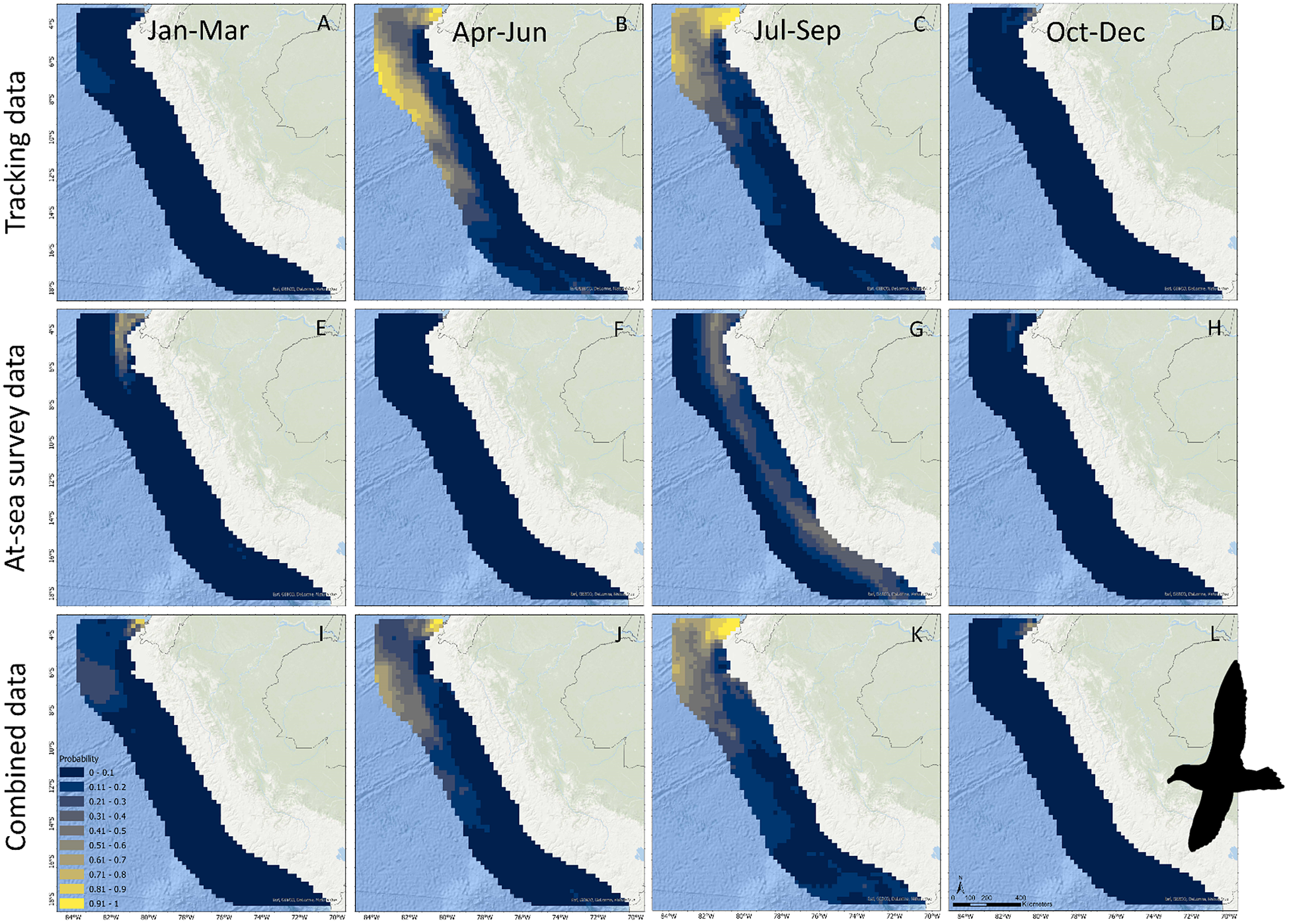
Figure 4. Predictions of Black Petrel occurrence in Peruvian waters based on tracking data (A–D), at-sea survey data (E–H), and both data sources combined (I–L). Note no at-sea surveys were conducted in July–September.
Influence of environmental variables
Environmental variables influenced occurrence predictions differently depending on the data used in our SDMs (Figure 5). For Salvin’s Albatross, tracking data showed that the probability of occurrence was negatively influenced by northern current velocity, SST, and distance to outer shelf, i.e. Salvin’s Albatrosses in Peru favoured cold, slow flowing waters close to the outer shelf. These results contrast with estimates based on at-sea survey data, which showed that probability of occurrence had a positive relationship with eastern current velocity and a quadratic relationship with turbidity. Thus, at-sea survey data suggested that Salvin’s Albatrosses favour faster flowing waters at a turbidity optimum. When modelling Salvin’s Albatross occurrence using both data combined, important interactions with environmental variables were negative relationships with northern current velocity, distance to outer shelf, and a potential quadratic relationship with turbidity. Therefore, combined data suggested that Salvin’s Albatrosses favoured cold, slow flowing waters close to the outer shelf, potentially at a turbidity optimum.
Tracking data for Black Petrels showed that the probability of occurrence had a negative relationship with eastern current velocity and bathymetry, a positive relationship with SST, and a quadratic relationship with turbidity. Tracking data thus suggested that Black Petrels in Peru favoured deep, warm, slow flowing waters, at a turbidity optimum. At-sea survey data showed that the probability of Black Petrel occurrence had a negative relationship with salinity and distance to outer shelf and a positive relationship with bathymetry, i.e. Black Petrels favoured shallow waters near the outer shelf with low salinity. When modelling Black Petrel occurrence using both data sources combined, important interactions with environmental variables were negative relationships with eastern current velocity, salinity, and bathymetry, positive relationships with SST and distance to outer shelf, and a quadratic relationship with turbidity. Combined data thus suggested that Black Petrels favoured deep, warm, slow flowing waters, with low salinity, at a turbidity optimum.

Figure 5. Estimates of coefficients used to estimate occurrence of Salvin’s Albatrosses (A) and Black Petrels (B) in Peruvian waters, using different presence-absence data sources. All environmental coefficients indicate year-round relationships (black symbols), while seasonal effects are modelled using separate coefficients (coloured symbols). Translucent symbols indicate CIs include zero.
Discussion
Using tracking or at-sea survey data independently in our SDMs showed seasonal differences in estimates of species occurrence and distribution and contrasting interactions with environmental variables, while combining both data sources resolved spatiotemporal imperfections, provided more balanced estimates, and reduced uncertainty. Inferences from tracking data showed that Salvin’s Albatrosses and Black Petrels occurred in Peruvian waters during February–July and April–October, respectively, while inferences from at-sea survey data showed that occurrences extended from February to November and from February to October for Salvin’s Albatross and Black Petrel, respectively. Tracking data highlighted different hotspots of relatively high occurrence when compared with at-sea survey data (seasonal occurrence in northern Peruvian waters for Salvin’s Albatross and seasonal occurrence in the Peru Basin for Black Petrels). Underlying these differences are contrasting estimates of interactions with environmental variables based on the data source used. Combining both data sources resulted in more balanced estimates of occurrence, distribution, and habitat selection. Most notably, combining both data sources predicted occurrence of both species in Peruvian waters during all four annual quarters (in the northern Humboldt upwelling system for Salvin’s Albatross and the equatorial and tropical superficial waters in northern Peru over the continental shelf for Black Petrels).
The differences between tracking-based and survey-based results may be caused by ontogenic biases in tracking data. Tracking studies usually focus on breeding adults (e.g. Peron and Gremillet Reference Peron and Gremillet2013), as was the case in our study. The higher occurrence of both species in Peruvian waters during April–September is a likely consequence of the seasonal migrations of breeding adults from Aotearoa to South America (Spear et al. Reference Spear, Ainley and Webb2003, Quinones et al. 2021). However, juveniles and non-breeding adults account for 47–81% of Procellariiform seabird populations (Carneiro et al. Reference Carneiro, Pearmain, Oppel, Clay, Phillips and Bonnet-Lebrun2020). Excluding these life-cycle stages from tracking can bias occurrence and distribution estimates. We observed predominantly subadult Salvin’s Albatrosses during October–November, which suggests that life-cycle stages, other than breeding adults, utilise Peruvian waters at different times. Consequently, ontogenic biases in tracking data may have caused our contrasting results. Our study thus highlights the importance of tracking life-cycle stages beyond breeding adults (de Grissac et al. Reference De Grissac, Borger, Guitteaud and Weimerskirch2016, Carneiro et al. Reference Carneiro, Pearmain, Oppel, Clay, Phillips and Bonnet-Lebrun2020, Frankish et al. Reference Frankish, Cunningham, Manica, Clay, Prince and Phillips2021). Once other life-cycle stages have been tracked, future research could repeat our efforts and provide separate estimates for both adults and subadults. Additionally, as our estimates were only quarterly, future research should quantify occurrence and distribution of these species in Peruvian waters at a higher temporal resolution (e.g. monthly).
The differences between tracking-based and survey-based results could also be explained by geographical biases in both data sources. Seabirds can exhibit inter-colony segregation in non-breeding areas (Gutowsky et al. Reference Gutowsky, Leonard, Conners, Shaffer and Jonsen2015, Bolton et al. Reference Bolton, Conolly, Carroll, Wakefield and Caldow2018). Yet, tracking studies often track birds from a single breeding colony (i.e. the largest or the most accessible colony), as was the case in our study. Single colony tracking studies can bias occurrence and distribution estimates (e.g. Rayner et al. Reference Rayner, Hauber, Steeves, Lawrence, Thompson and Sagar2011). There is evidence suggesting that Salvin’s Albatrosses exhibit inter-colony segregation at their non-breeding distribution. Birds from the relatively small Tine Heke colony may potentially migrate further north than birds from the larger Hauriri colony (Thompson et al. Reference Thompson, Sagar, Torres and Charteris2014). However, it should be noted that this evidence is based on GLS tracking only. The contrasts between GLS and PTT/GPS tracks in our study (Figure 1) suggested that Salvin’s Albatross GLS tracks may be subject to local idiosyncrasies in accuracy (Halpin et al. Reference Halpin, Ross, Ramos, Mott, Carlile and Golding2021), despite our best efforts to correct for these (Merkel et al. Reference Merkel, Phillips, Descamps, Yoccoz, Moe and Strom2016), and these idiosyncrasies should be further investigated. No evidence for inter-colony segregation exists for Black Petrels (Bell et al. Reference Bell, Sim, Abraham, Torres and Shaffer2014). Our results thus also support the need for multi-colony tracking studies. Inversely, while our effort was highly comparable between surveys, effort was concentrated on waters within 120 nm (222 km) from shore, due to logistical constraints. This limitation could have also biased survey results to inshore waters, which, for example, could explain the lack of estimated occurrence of Black Petrels in the Peru Basin. Our results thus also highlight the need for ocean-wide at-sea surveys (Priddel et al. Reference Priddel, Carlile, Portelli, Kim, O’Neill and Bretagnolle2014).
Peruvian waters form an important part of the distribution of these two vulnerable seabirds. Both species migrate >7,000 km from their breeding colonies in Aotearoa to Peruvian waters and utilise these waters during different life-cycle stages. It is likely that the high productivity in Peruvian waters attracts these birds, and the relationships of both species with turbidity, current velocity, and distance to shelf supported this. The cold waters of the Northern Humboldt Current that dominate Peruvian waters are highly productive. In fact, this area is the most productive eastern boundary current system worldwide (Paulik Reference Paulik, Glantz and Thompson1981, Spear et al. Reference Spear, Ainley and Webb2003, Chavez et al. Reference Chavez, Bertrand, Guevara-Carrasco, Soler and Csirke2008). Additionally, eddy-like structures occur in southern Peruvian offshore waters (from -15° S to -17° S), extending the high primary productivity to offshore waters (Chaigneau et al. Reference Chaigneau, Gizolme and Grados2008, Reference Chaigneau, Dominguez, Eldin, Vasquez, Flores and Grados2013). The high productivity results in heightened zooplankton concentrations and increased abundances of prey species such as squid (e.g. Abraliopsis sp., Argonauta nouryi, and Dosidicus gigas) and fish (e.g. Trachurus sp., Vinciguerria sp.) (Acha et al. Reference Acha, Piola, Iribarne and Mianzan2015, Quiñones et al. Reference Quiñones, Calderon, Mayaute and Bell2020, Reference Quiñones, Alegre, Romero, Manrique and Vasquez2021). Consequently, the highly productive waters off Peru sustain these two seabirds from Aotearoa. However, these highly productive Peruvian waters are also characterised by high inter-annual climatic fluctuations (e.g. Chavez et al. Reference Chavez, Bertrand, Guevara-Carrasco, Soler and Csirke2008). Here, we used only three years of tracking and survey data, which were not sufficient to account for inter-annual variation. Therefore, the continuation of tracking and simultaneous at-sea surveys would improve insights into inter-annual variations.
Robust, year-round insights into the distribution and occurrence of vulnerable seabirds are crucial for their conservation. Salvin’s Albatrosses and Black Petrels are highly vulnerable to bycatch in commercial trawl, pelagic longline, and demersal longline fisheries, in their breeding ranges surrounding Aotearoa, mainly due to industrial fisheries (Richard et al. Reference Richard, Abraham and Berkenbusch2020), and their non-breeding ranges in South America, due to both industrial and artisanal fisheries (Abraham et al. Reference Abraham, Richard, Walker, Gibson, Ochi and Tsuji2019, Moreno and Quiñones Reference Moreno and Quiñones2022). In Aotearoa, estimates of seabird distribution and occurrence are overlaid with fishing effort to assess risks and prioritise conservation efforts (e.g. Richard et al. Reference Richard, Abraham and Berkenbusch2020). However, such exercises are rare for the non-breeding ranges of species traversing entire ocean basins (Clay et al. Reference Clay, Small, Tuck, Pardo, Carneiro and Wood2019). Despite some shortcomings, we here provide estimates of the distribution and occurrence of Salvin’s Albatross and Black Petrel in their non-breeding range within Peruvian waters. These estimates will facilitate future overlap analyses with commercial (e.g. Kroodsma et al. Reference Kroodsma, Mayorga, Hochberg, Miller, Boerder and Ferretti2018), and potentially, artisanal longline fishing effort in Peruvian waters (Majluf et al. Reference Majluf, Babcock, Riveros, Schreiber and Alderete2002, Doherty et al. Reference Doherty, Shigueto, Hodgson, Mangel, Witt and Godley2014). Such overlap analyses will allow non-breeding distribution risk assessments and, ultimately, could improve the efficacy of future conservation actions for both species (e.g. targeted promotion of best practice mitigation measures) (ACAP 2021a,b).
Our results highlight the value of using multiple data sources to overcome imperfections and biases prevalent in single data sources. Combining seabird tracking with at-sea surveys allowed us to overcome potential ontogenic and geographical biases in either data source, resulting in more robust occurrence and distribution estimates. Fusing data sources highlighted the importance of Peruvian waters for Salvin’s Albatrosses and Black Petrels during all four annual quarters. These insights will prove invaluable for future non-breeding distribution risk assessments and conservation actions for these species. As such, our study exemplifies how trans-oceanic collaborations can provide more robust guidance for seabird conservation throughout their distribution and annual cycles.
Acknowledgements
MC, GCP, KRH, PMS, and DRT thank Steve Kafka, Jim Dilley, and the entire crew of the Evohe for safe passage to and from Hauriri and the staff of the DOC Murihiku office for biosecurity and logistical support. PC, SR, and EB thank Ngāti Rehua Ngāti Wai ki Aotea for their ongoing support and permission to carry out this work, L. Mack, the staff of the DOC Okiwi office, S. Matthews, and C. Matthews for logistical support, and J. Ranstead, A. Clow, L. Clow, the crew of the Southern Cross, J. Molloy, J. Gower, J. Walter, D. Lees, G. Hobson, J. Dolton, S. van Leeuwen, and H. Ricardo, for assistance in the field on Aotea. CM and JQ thank C. Moreno, M. Manrique, L. Mayaute, J. Calderon, and S. Falero for assisting with at-sea surveys and the skippers and crew of the Humboldt and the Jose Olaya Balandra for their safe navigation of Peruvian waters. All fieldwork in Aotearoa was carried out with permission from local iwi (Kaitiaki Rōpū ki Murihiku and Ngāi Tahu for Hauriri, Ngāti Rehua Ngāti Wai ki Aotea for Aotea), the New Zealand Department of Conservation (M1819/04 for Hauriri), and Animal Ethics Committees (Gummer Reference Gummer2013a, Reference Gummerb for Hauriri, AEC321 for Aotea). Fieldwork on Hauriri was funded by the Conservation Services Program of the New Zealand Department of Conservation (POP2017-03). Fieldwork on Aotea was funded by the New Zealand Ministry of Primary Industries (PRO2017-01A). At-sea surveys in Peruvian waters were funded by the Instituto del Mar del Perú.
Supplementary Materials
To view supplementary material for this article, please visit http://doi.org/10.1017/S0959270922000442.


