


1. Introduction and main results
In 1957, Broadbent and Hammersley [Reference Broadbent and Hammersley6] initiated the study of percolation theory in order to model the flow of fluid through a medium with randomly blocked channels. In (bond) percolation, given a graph
 $G$
, the percolated random subgraph
$G$
, the percolated random subgraph
 $G_p$
is obtained by retaining every edge of the host graph
$G_p$
is obtained by retaining every edge of the host graph
 $G$
independently and with probability
$G$
independently and with probability
 $p$
. If we take the host graph
$p$
. If we take the host graph
 $G$
to be the complete graph
$G$
to be the complete graph
 $K_{d+1}$
then
$K_{d+1}$
then
 $G_p$
coincides with the well-known binomial random graph model
$G_p$
coincides with the well-known binomial random graph model
 $G(d+1,p)$
. In their seminal paper from 1960, Erdős and Rényi [Reference Erdős and Rényi12] showed that
$G(d+1,p)$
. In their seminal paper from 1960, Erdős and Rényi [Reference Erdős and Rényi12] showed that
 $G(d+1,p)$
Footnote 1 undergoes a dramatic phase transition, with respect to its component structure, when
$G(d+1,p)$
Footnote 1 undergoes a dramatic phase transition, with respect to its component structure, when
 $p$
is around
$p$
is around
 $\frac{1}{d}$
. More precisely, given a constant
$\frac{1}{d}$
. More precisely, given a constant
 $\epsilon \gt 0$
let us define
$\epsilon \gt 0$
let us define
 $y=y(\epsilon )$
to be the unique solution in
$y=y(\epsilon )$
to be the unique solution in
 $(0,1)$
of the equation
$(0,1)$
of the equation
 \begin{align} y=1-\exp \left (-(1+\epsilon )y\right ), \end{align}
where we note that
 $y$
is an increasing continuous function on
$y$
is an increasing continuous function on
 $(0,\infty )$
with
$(0,\infty )$
with
 $y(\epsilon ) = 2\epsilon - O(\epsilon ^2)$
.
$y(\epsilon ) = 2\epsilon - O(\epsilon ^2)$
.
Theorem 1 ([Reference Erdős and Rényi12]). Let
 $\epsilon \gt 0$
be a small enough constant. Then, with probability tending to one as
$\epsilon \gt 0$
be a small enough constant. Then, with probability tending to one as
 $d \to \infty$
,
$d \to \infty$
,
-
(a) if
 $p=\frac{1-\epsilon }{d}$
, then all the components of
$G(d+1,p)$
are of order
$O_{\epsilon }\left (\log d \right )$
; and,
$p=\frac{1-\epsilon }{d}$
, then all the components of
$G(d+1,p)$
are of order
$O_{\epsilon }\left (\log d \right )$
; and,
-
(b) if
$p=\frac{1+\epsilon }{d}$
, then there exists a unique giant component in
$G(d+1,p)$
of order
$(1+o(1))y(\epsilon )d$
. Furthermore, all the other components of
$G(d+1,p)$
are of order
$O_{\epsilon }\left (\log d\right )$
.


We refer the reader to [Reference Bollobás3, Reference Frieze and Karoński14, Reference Janson, Łuczak and Ruciński17] for a systematic coverage of random graphs, and to the monographs [Reference Bollobás and Riordan5, Reference Grimmett15, Reference Kesten18] on percolation theory.
This phenomenon of such a sharp change in the order of the largest component has been subsequently studied in many other percolation models. Some well-studied examples come from percolation on lattice-like structures with fixed dimension (see [Reference Heydenreich and van der Hofstad16] for a survey on many results in this subject). Another extensively studied model is the percolated hypercube, where the host graph is the
 $d$
-dimensional hypercube
$d$
-dimensional hypercube
 $Q^d$
. Indeed, answering a question of Erdős and Spencer [Reference Erdős and Spencer13], Ajtai, Komlós, and Szemerédi [Reference Ajtai, Komlós and Szemerédi1] proved that
$Q^d$
. Indeed, answering a question of Erdős and Spencer [Reference Erdős and Spencer13], Ajtai, Komlós, and Szemerédi [Reference Ajtai, Komlós and Szemerédi1] proved that
 $Q^d_p$
undergoes a phase transition quantitatively similar to the one which occurs in
$Q^d_p$
undergoes a phase transition quantitatively similar to the one which occurs in
 $G(d+1,p)$
, and their work was later extended by Bollobás, Kohayakawa, and Łuczak [Reference Bollobás, Kohayakawa and Łuczak4].
$G(d+1,p)$
, and their work was later extended by Bollobás, Kohayakawa, and Łuczak [Reference Bollobás, Kohayakawa and Łuczak4].
Theorem 2 ([Reference Ajtai, Komlós and Szemerédi1, Reference Bollobás, Kohayakawa and Łuczak4]). Let
 $\epsilon \gt 0$
be a small enough constant. Then, with probability tending to one as
$\epsilon \gt 0$
be a small enough constant. Then, with probability tending to one as
 $d \to \infty$
,
$d \to \infty$
,
-
(a) if
$p=\frac{1-\epsilon }{d}$
, then all the components of
$Q^d_p$
are of order
$O_{\epsilon }(d)$
; and,
-
(b) if
$p=\frac{1+\epsilon }{d}$
, then there exists a unique giant component of order
$(1+o(1))y(\epsilon )2^d$
. Furthermore, all the other components of
$Q^d_p$
are of order
$O_{\epsilon }(d)$
.


Note that, since
 $|V(Q^d)| = 2^d$
, in both Theorems 1 and 2 the likely order of the largest component changes from logarithmic in the order of the host graph in the subcritical regime, to linear in the order of the host graph in the supercritical regime, whilst the second-largest component in the supercritical regime remains of logarithmic order. Furthermore, in both models this giant component is the unique component of linear order, and covers the same asymptotic fraction of the vertices in each case. We informally refer to this quantitative behaviour as the Erdős-Rényi component phenomenon.
$|V(Q^d)| = 2^d$
, in both Theorems 1 and 2 the likely order of the largest component changes from logarithmic in the order of the host graph in the subcritical regime, to linear in the order of the host graph in the supercritical regime, whilst the second-largest component in the supercritical regime remains of logarithmic order. Furthermore, in both models this giant component is the unique component of linear order, and covers the same asymptotic fraction of the vertices in each case. We informally refer to this quantitative behaviour as the Erdős-Rényi component phenomenon.
Recently, Lichev [Reference Lichev19] initiated the study of percolation on some families of high-dimensional graphs, those arising from the product of many bounded-degree graphs. Given a sequence of graphs
 $G^{(1)},\ldots, G^{(t)}$
, the Cartesian product of
$G^{(1)},\ldots, G^{(t)}$
, the Cartesian product of
 $G^{(1)},\ldots, G^{(t)}$
, denoted by
$G^{(1)},\ldots, G^{(t)}$
, denoted by
 $G=G^{(1)}\square \cdots \square G^{(t)}$
or
$G=G^{(1)}\square \cdots \square G^{(t)}$
or
 $G=\square _{i=1}^{t}G^{(i)}$
, is the graph with the vertex set
$G=\square _{i=1}^{t}G^{(i)}$
, is the graph with the vertex set
 \begin{align*} V(G)=\left \{v=(v_1,v_2,\ldots,v_t) \colon v_i\in V(G^{(i)}) \text{ for all } i \in [t]\right \}, \end{align*}
and the edge set
 \begin{align*} E(G)=\left \{uv \colon \begin{array}{l} \text{there is some } i\in [t] \text{ such that } u_iv_i\in E\left (G^{(i)}\right )\\[5pt] \text{ and } u_j=v_j \text{ for all } i \neq j \end{array}\right \}. \end{align*}
We call
 $G^{(i)}$
the base graphs of
$G^{(i)}$
the base graphs of
 $G$
. Throughout the rest of the paper, we denote by
$G$
. Throughout the rest of the paper, we denote by
 $|G|$
the number of vertices of the graph
$|G|$
the number of vertices of the graph
 $G$
, and use
$G$
, and use
 $t$
for the number of base graphs in the product. We denote by
$t$
for the number of base graphs in the product. We denote by
 $d\;:\!=\; d(G)$
the average degree of a given graph
$d\;:\!=\; d(G)$
the average degree of a given graph
 $G$
.
$G$
.
Considering percolation in these high-dimensional product graphs, Lichev [Reference Lichev19] showed the existence of a threshold for the appearance of a component of linear order in these models, under some mild assumptions on the isoperimetric constants of the base graphs. The isoperimetric constant
 $i(H)$
of a graph
$i(H)$
of a graph
 $H$
is a measure of the edge-expansion of
$H$
is a measure of the edge-expansion of
 $H$
and is given by
$H$
and is given by
 \begin{equation*} i(H)=\min _{\begin {subarray}{c}S\subseteq V(H),\\[5pt] |S|\le |V(H)|/2\end {subarray}}\frac {e(S, S^C)}{|S|}. \end{equation*}
Throughout the paper, all asymptotics are with respect to
 $t$
, and we use the standard Landau notations (see e.g., [Reference Janson, Łuczak and Ruciński17]). We often state results for properties that hold whp, (short for “with high probability”), that is, with probability tending to
$t$
, and we use the standard Landau notations (see e.g., [Reference Janson, Łuczak and Ruciński17]). We often state results for properties that hold whp, (short for “with high probability”), that is, with probability tending to
 $1$
as
$1$
as
 $t$
tends to infinity.
$t$
tends to infinity.
Theorem 3 ([Reference Lichev19]). Let
 $C, \gamma \gt 0$
be constants and let
$C, \gamma \gt 0$
be constants and let
 $\epsilon \gt 0$
be a small enough constant. Let
$\epsilon \gt 0$
be a small enough constant. Let
 $G^{(1)},\ldots, G^{(t)}$
be graphs such that
$G^{(1)},\ldots, G^{(t)}$
be graphs such that
 $1\le \Delta \left (G^{(j)}\right )\le C$
and
$1\le \Delta \left (G^{(j)}\right )\le C$
and
 $i\left (G^{(j)}\right )\ge t^{-\gamma }$
for all
$i\left (G^{(j)}\right )\ge t^{-\gamma }$
for all
 $j\in [t]$
. Let
$j\in [t]$
. Let
 $G=\square _{j=1}^{t}G^{(j)}$
. Then,
whp
$G=\square _{j=1}^{t}G^{(j)}$
. Then,
whp
-
1. if
$p=\frac{1-\epsilon }{d}$
, then all the components of
$G_p$
are of order at most
$\exp \left (-\frac{\epsilon ^2t}{9C^2}\right )|G|$
; -
2. if
$p=\frac{1+\epsilon }{d}$
, then there exists a positive constant
$c_1=c_1(\epsilon,C,\gamma )$
such that the largest component of
$G_p$
is of order at least
$c_1|G|$
.


Lichev asked if the conditions in Theorem 3 could be weakened.
Question 4 ([Reference Lichev19, Question 5.1]). Does Theorem
3 still hold without the assumption on the maximum degrees of the
 $G^{(j)}\mathord{?}$
Question 5 ([Reference Lichev19, Question 5.2]). Does Theorem
3 still hold if the isoperimetric constant
 $i\left (G^{(j)}\right )$
decreases faster than a polynomial function of
$i\left (G^{(j)}\right )$
decreases faster than a polynomial function of
 $t\mathord{?}$
Furthermore, in comparison to Theorems 1 and 2, we note that Theorem 3 only gives a rough, qualitative description of the phase transition, and it is natural to ask if a more precise, quantitative description of the component structure of these percolated product graphs in the sub- and supercritical regimes can be given, in the vein of the Erdős-Rényi component phenomenon, and if not in general, then under which additional assumptions?
In a recent paper [Reference Diskin, Erde, Kang and Krivelevich9], the authors gave a partial answer to this final question, showing that it is sufficient to assume that the base graphs are all regular and of bounded order.
Theorem 6 (Informal [Reference Diskin, Erde, Kang and Krivelevich9]). Let
 $C\gt 1$
be a constant and let
$C\gt 1$
be a constant and let
 $G=\square _{j=1}^{t}G^{(j)}$
be a product graph where
$G=\square _{j=1}^{t}G^{(j)}$
be a product graph where
 $G^{(j)}$
is connected and regular and
$G^{(j)}$
is connected and regular and
 $1 \lt \left |V\left (G^{(j)}\right )\right | \leq C$
for each
$1 \lt \left |V\left (G^{(j)}\right )\right | \leq C$
for each
 $j \in [t]$
. Then
$j \in [t]$
. Then
 $G_p$
undergoes a phase transition around
$G_p$
undergoes a phase transition around
 $p=\frac{1}{d}$
, which exhibits the Erdős-Rényi component phenomenon.
$p=\frac{1}{d}$
, which exhibits the Erdős-Rényi component phenomenon.
In this paper, we will investigate further the properties of the phase transition in irregular high-dimensional product graphs. Firstly, we will give a negative answer to Question 4, showing that if the maximum degree of the base graphs is allowed to grow (as a function in
 $t$
), then the largest component may have sublinear order for any
$t$
), then the largest component may have sublinear order for any
 $p = \Theta \left (\frac{1}{d}\right )$
. Let us write
$p = \Theta \left (\frac{1}{d}\right )$
. Let us write
 $S(r,s)$
for the graph formed by taking the complete graph
$S(r,s)$
for the graph formed by taking the complete graph
 $K_{r}$
on
$K_{r}$
on
 $r$
vertices and adding
$r$
vertices and adding
 $s$
leaves to each vertex of
$s$
leaves to each vertex of
 $K_r$
.
$K_r$
.
Theorem 7.
Let
 $r=r(t)$
and
$r=r(t)$
and
 $s=s(t)$
be integers, which may tend to infinity as
$s=s(t)$
be integers, which may tend to infinity as
 $t$
tends to infinity, such that
$t$
tends to infinity, such that
 $r = \omega (s t)$
. Let
$r = \omega (s t)$
. Let
 $G^{(j)}=K_2$
for
$G^{(j)}=K_2$
for
 $1\leq j \lt t$
, let
$1\leq j \lt t$
, let
 $G^{(t)} = S(r,s)$
and let
$G^{(t)} = S(r,s)$
and let
 $G=\square _{i=1}^t G^{(i)}$
, where we note that
$G=\square _{i=1}^t G^{(i)}$
, where we note that
 $d = (1+o(1))\frac{r}{s}$
. Let
$d = (1+o(1))\frac{r}{s}$
. Let
 $p\le \frac{1}{4st}$
. Then,
whp
the largest component of
$p\le \frac{1}{4st}$
. Then,
whp
the largest component of
 $G_p$
has order at most
$G_p$
has order at most
 $\frac{2|G|}{s}$
.
$\frac{2|G|}{s}$
.
Note that for the base graphs defined in Theorem 7, we have
 $i\left (G^{(j)}\right )=1$
for
$i\left (G^{(j)}\right )=1$
for
 $1\le j \le t-1$
, and
$1\le j \le t-1$
, and
 $i\left (G^{(t)}\right )=\Omega \left (\frac{1}{s}\right )$
, and so, as long as
$i\left (G^{(t)}\right )=\Omega \left (\frac{1}{s}\right )$
, and so, as long as
 $s$
is not too large, this graph will satisfy the requirements of Theorem 3 regarding the isoperimetric constant. However, by choosing
$s$
is not too large, this graph will satisfy the requirements of Theorem 3 regarding the isoperimetric constant. However, by choosing
 $s = \omega (1)$
and
$s = \omega (1)$
and
 $r = \omega ( s^2t)$
, so that the upper bound on the edge probability
$r = \omega ( s^2t)$
, so that the upper bound on the edge probability
 $p$
in Theorem 7 is such that
$p$
in Theorem 7 is such that
 $\frac{1}{4st} = \omega \left (\frac{s}{r}\right ) = \omega \left ( \frac{1}{d}\right )$
, we see that even significantly above the point
$\frac{1}{4st} = \omega \left (\frac{s}{r}\right ) = \omega \left ( \frac{1}{d}\right )$
, we see that even significantly above the point
 $p_* = \frac{1}{d}$
, the largest component in the percolated product graph will typically have size
$p_* = \frac{1}{d}$
, the largest component in the percolated product graph will typically have size
 $o(|G|)$
. The key observation in the construction is that most vertices in
$o(|G|)$
. The key observation in the construction is that most vertices in
 $G$
have degree
$G$
have degree
 $t$
while
$t$
while
 $d\gg t$
. Thus, these vertices are likely to be isolated for
$d\gg t$
. Thus, these vertices are likely to be isolated for
 $p$
which is around
$p$
which is around
 $\frac{1}{d}$
.
$\frac{1}{d}$
.
However, we are able to give a positive answer to Question 5, showing that in fact a threshold for the existence of a linear sized component in a percolated product graph exists even when the isoperimetric constants of the base graphs are super-exponentially small in
 $t$
. Furthermore, we strengthen Lichev’s [Reference Lichev19] result by determining the asymptotic order of the giant, and showing that it is in fact unique.
$t$
. Furthermore, we strengthen Lichev’s [Reference Lichev19] result by determining the asymptotic order of the giant, and showing that it is in fact unique.
Theorem 8.
Let
 $C\gt 0$
be a constant, and let
$C\gt 0$
be a constant, and let
 $\epsilon \gt 0$
be a small enough constant. Let
$\epsilon \gt 0$
be a small enough constant. Let
 $G^{(1)},\ldots, G^{(t)}$
be graphs such that for all
$G^{(1)},\ldots, G^{(t)}$
be graphs such that for all
 $j\in [t]$
,
$j\in [t]$
,
 $1\le \Delta \left (G^{(j)}\right )\le C$
and
$1\le \Delta \left (G^{(j)}\right )\le C$
and
 $i\left (G^{(j)}\right )\ge t^{-t^{\frac{1}{4}}}$
. Let
$i\left (G^{(j)}\right )\ge t^{-t^{\frac{1}{4}}}$
. Let
 $G=\square _{j=1}^{t}G^{(j)}$
, let
$G=\square _{j=1}^{t}G^{(j)}$
, let
 $d$
be the average degree of
$d$
be the average degree of
 $G$
and let
$G$
and let
 $p=\frac{1+\epsilon }{d}$
. Then,
whp
$p=\frac{1+\epsilon }{d}$
. Then,
whp
-
(a)
$G_p$
contains a unique giant component of order
$(1+o(1))y(\epsilon )|G|$
, where
$y(\epsilon )$
is defined according to (1); -
(b) all other components of
$G_p$
are of order
$o(|G|)$
.


Note that, this is the same asymptotic fraction of the vertices as in Theorems 1 and 2.
Whilst Theorem 8 concerns the size of the largest component in the supercritical regime, which follows the Erdős-Rényi component phenomenon, we are also able to give an example that demonstrates that, if the base graphs are allowed to be irregular, the percolated product graph can also significantly deviate in behaviour from the Erdős-Rényi component phenomenon in the subcritical regime.
Theorem 9.
Let
 $s$
be a large enough integer. Let
$s$
be a large enough integer. Let
 $G^{(i)}=S(1,s)$
, that is, a star with
$G^{(i)}=S(1,s)$
, that is, a star with
 $s$
leaves, for every
$s$
leaves, for every
 $1\le i \le t$
, and let
$1\le i \le t$
, and let
 $G=\square _{i=1}^tG^{(i)}$
, noting that
$G=\square _{i=1}^tG^{(i)}$
, noting that
 $d = \frac{2st}{s+1}$
. Let
$d = \frac{2st}{s+1}$
. Let
 $p= \frac{c}{t}$
for
$p= \frac{c}{t}$
for
 $c\gt \frac{1}{3}$
. Then,
whp
the largest component of
$c\gt \frac{1}{3}$
. Then,
whp
the largest component of
 $G_p$
is of order at least
$G_p$
is of order at least
 $|G|^{1-s^{-\frac{1}{6}}}$
.
$|G|^{1-s^{-\frac{1}{6}}}$
.
Note that Theorem 9 demonstrates the necessity of the assumption that the base graphs are regular in Theorem 6, as well as the near optimality of the bound in Theorem 3 (a), in terms of the size of the largest component in the subcritical regime. Indeed, since
 $t = \Theta (\log |G|)$
and
$t = \Theta (\log |G|)$
and
 $ \Delta \left (G^{(i)}\right ) = s = \Theta (1)$
for all
$ \Delta \left (G^{(i)}\right ) = s = \Theta (1)$
for all
 $i$
, here we have that the largest component has order at least
$i$
, here we have that the largest component has order at least
 $\exp \left (-\Theta ( t) \right ) |G|$
, which matches the bound in Theorem 3 (a), up to the dependence on
$\exp \left (-\Theta ( t) \right ) |G|$
, which matches the bound in Theorem 3 (a), up to the dependence on
 $p$
and
$p$
and
 $\max _i \{\Delta \left (G^{(i)}\right ) \}$
in the leading constant. Furthermore, note that as
$\max _i \{\Delta \left (G^{(i)}\right ) \}$
in the leading constant. Furthermore, note that as
 $s$
grows, the bound on the largest component grows close to linear in
$s$
grows, the bound on the largest component grows close to linear in
 $|G|$
.
$|G|$
.
The structure of the paper is as follows. In Section 2 we introduce some preliminary tools and lemmas we will use in the paper. In Section 3 we give a (short) proof for Theorem 7. In Section 4 we provide a general framework for showing the existence of a large component, in particular in high-dimensional product graphs. We then use this framework to prove Theorem 8 and, with an additional analysis of the structure of the
 $t$
-fold product of stars, to prove Theorem 9, where the proofs of these two theorems are the most involved part of the paper. Finally, in Section 5 we make some brief comments on our results and indicate directions for further research.
$t$
-fold product of stars, to prove Theorem 9, where the proofs of these two theorems are the most involved part of the paper. Finally, in Section 5 we make some brief comments on our results and indicate directions for further research.
2. Preliminaries
With respect to high-dimensional product graphs, our notation follows that of [Reference Diskin, Erde, Kang and Krivelevich9]. Given a vertex
 $u = (u_1,u_2, \ldots, u_t)$
in
$u = (u_1,u_2, \ldots, u_t)$
in
 $V(G)$
and
$V(G)$
and
 $i \in [t]$
we call the vertex
$i \in [t]$
we call the vertex
 $u_i\in V\left (G^{(i)}\right )$
the
$u_i\in V\left (G^{(i)}\right )$
the
 $i$
th coordinate of
$i$
th coordinate of
 $u$
. We note that, as is standard, we may still enumerate the vertices of a given set
$u$
. We note that, as is standard, we may still enumerate the vertices of a given set
 $M$
, such as
$M$
, such as
 $M=\left \{v_1,\ldots, v_m\right \}$
with
$M=\left \{v_1,\ldots, v_m\right \}$
with
 $v_i\in V(G)$
. Whenever confusion may arise, we will clarify whether the subscript stands for enumeration of the vertices of the set, or for their coordinates.
$v_i\in V(G)$
. Whenever confusion may arise, we will clarify whether the subscript stands for enumeration of the vertices of the set, or for their coordinates.
When
 $G^{(i)}$
is a graph on a single vertex, that is,
$G^{(i)}$
is a graph on a single vertex, that is,
 $G^{(i)}=\left (\{u\},\varnothing \right )$
, we call it trivial (and non-trivial, otherwise). We define the dimension of
$G^{(i)}=\left (\{u\},\varnothing \right )$
, we call it trivial (and non-trivial, otherwise). We define the dimension of
 $G=\square _{i=1}^tG^{(i)}$
to be the number of base graphs
$G=\square _{i=1}^tG^{(i)}$
to be the number of base graphs
 $G^{(i)}$
of
$G^{(i)}$
of
 $G$
which are non-trivial.
$G$
which are non-trivial.
Given
 $H\subseteq G=\square _{i=1}^tG^{(i)}$
, we call
$H\subseteq G=\square _{i=1}^tG^{(i)}$
, we call
 $H$
a projection of
$H$
a projection of
 $G$
if
$G$
if
 $H$
can be written as
$H$
can be written as
 $H=\square _{i=1}^tH^{(i)}$
where for every
$H=\square _{i=1}^tH^{(i)}$
where for every
 $1\le i\le t$
,
$1\le i\le t$
,
 $H^{(i)}=G^{(i)}$
or
$H^{(i)}=G^{(i)}$
or
 $H^{(i)}=\{v_i\}\subseteq V\left (G^{(i)}\right )$
; that is,
$H^{(i)}=\{v_i\}\subseteq V\left (G^{(i)}\right )$
; that is,
 $H$
is a projection of
$H$
is a projection of
 $G$
if it is the Cartesian product graph of base graphs
$G$
if it is the Cartesian product graph of base graphs
 $G^{(i)}$
and their trivial subgraphs. In that case, we further say that
$G^{(i)}$
and their trivial subgraphs. In that case, we further say that
 $H$
is the projection of
$H$
is the projection of
 $G$
onto the coordinates corresponding to the trivial subgraphs. For example, let
$G$
onto the coordinates corresponding to the trivial subgraphs. For example, let
 $u_i\in V\left (G^{(i)}\right )$
for
$u_i\in V\left (G^{(i)}\right )$
for
 $1\le i\le k$
, and let
$1\le i\le k$
, and let
 $H=\{u_1\}\square \cdots \square \{u_k\}\square G^{(k+1)}\square \cdots \square G^{(t)}$
. In this case we say that
$H=\{u_1\}\square \cdots \square \{u_k\}\square G^{(k+1)}\square \cdots \square G^{(t)}$
. In this case we say that
 $H$
is a projection of
$H$
is a projection of
 $G$
onto the first
$G$
onto the first
 $k$
coordinates.
$k$
coordinates.
Given a graph
 $H$
and a vertex
$H$
and a vertex
 $v \in V(H)$
, we denote by
$v \in V(H)$
, we denote by
 $C_v(H)$
the component of
$C_v(H)$
the component of
 $v$
in
$v$
in
 $H$
. We denote by
$H$
. We denote by
 $N_H(S)$
the external neighbourhood of a set
$N_H(S)$
the external neighbourhood of a set
 $S$
in the graph
$S$
in the graph
 $H$
, by
$H$
, by
 $E_H(A,B)$
the set of edges between
$E_H(A,B)$
the set of edges between
 $A$
and
$A$
and
 $B$
in
$B$
in
 $H$
, and by
$H$
, and by
 $e_H(A,B)\;:\!=\; |E_H(A,B)|$
. When the graph we refer to is obvious, we may omit the subscript. We omit rounding signs for the sake of clarity of presentation.
$e_H(A,B)\;:\!=\; |E_H(A,B)|$
. When the graph we refer to is obvious, we may omit the subscript. We omit rounding signs for the sake of clarity of presentation.
2.1. The BFS algorithm
For the proofs of our main results, we will use the Breadth First Search (BFS) algorithm. This algorithm explores the components of a graph
 $G$
by building a maximal spanning forest.
$G$
by building a maximal spanning forest.
The algorithm receives as input a graph
 $G$
and a linear ordering
$G$
and a linear ordering
 $\sigma$
on its vertices. The algorithm maintains three sets of vertices:
$\sigma$
on its vertices. The algorithm maintains three sets of vertices:
-
•
$S$
, the set of vertices whose exploration is complete; -
•
$Q$
, the set of vertices currently being explored, kept in a queue; and -
•
$T$
, the set of vertices that have not been explored yet.


The algorithm starts with
 $S=Q=\emptyset$
and
$S=Q=\emptyset$
and
 $T=V(G)$
, and ends when
$T=V(G)$
, and ends when
 $Q\cup T=\emptyset$
. At each step, if
$Q\cup T=\emptyset$
. At each step, if
 $Q$
is non-empty, the algorithm queries the vertices in
$Q$
is non-empty, the algorithm queries the vertices in
 $T$
, in the order
$T$
, in the order
 $\sigma$
, to ascertain if they are neighbours in
$\sigma$
, to ascertain if they are neighbours in
 $G$
of the first vertex
$G$
of the first vertex
 $v$
in
$v$
in
 $Q$
. Each neighbour which is discovered is added to the back of the queue
$Q$
. Each neighbour which is discovered is added to the back of the queue
 $Q$
. Once all neighbours of
$Q$
. Once all neighbours of
 $v$
have been discovered, we move
$v$
have been discovered, we move
 $v$
from
$v$
from
 $Q$
to
$Q$
to
 $S$
. If
$S$
. If
 $Q=\emptyset$
, then we move the next vertex from
$Q=\emptyset$
, then we move the next vertex from
 $T$
(according to
$T$
(according to
 $\sigma$
) into
$\sigma$
) into
 $Q$
. Note that the set of edges queried during the algorithm forms a maximal spanning forest of
$Q$
. Note that the set of edges queried during the algorithm forms a maximal spanning forest of
 $G$
.
$G$
.
In order to analyse the BFS algorithm on a random subgraph
 $G_p$
of a graph
$G_p$
of a graph
 $G$
with
$G$
with
 $m$
edges, we will utilise the principle of deferred decisions. That is, we will take a sequence
$m$
edges, we will utilise the principle of deferred decisions. That is, we will take a sequence
 $(X_i \colon 1 \leq i \leq m)$
of i.i.d. Bernoulli
$(X_i \colon 1 \leq i \leq m)$
of i.i.d. Bernoulli
 $(p)$
random variables, which we will think of as representing a positive or negative answer to a query in the algorithm. When the
$(p)$
random variables, which we will think of as representing a positive or negative answer to a query in the algorithm. When the
 $i$
th edge of
$i$
th edge of
 $G$
is queried during the BFS algorithm, we will include it in
$G$
is queried during the BFS algorithm, we will include it in
 $G_p$
if and only if
$G_p$
if and only if
 $X_i=1$
. It is clear that the forest obtained in this way has the same distribution as a forest obtained by running the BFS algorithm on
$X_i=1$
. It is clear that the forest obtained in this way has the same distribution as a forest obtained by running the BFS algorithm on
 $G_p$
.
$G_p$
.
2.2. Preliminary lemmas
We will make use of two standard probabilistic bounds. The first is a typical Chernoff type tail bound on the binomial distribution (see, for example, Appendix A in [Reference Alon and Spencer2]).
Lemma 10.
Let
 $n\in \mathbb{N}$
, let
$n\in \mathbb{N}$
, let
 $p\in [0,1]$
, and let
$p\in [0,1]$
, and let
 $X\sim \text{Bin}(n,p)$
. Then for any positive
$X\sim \text{Bin}(n,p)$
. Then for any positive
 $m$
with
$m$
with
 $m\le \frac{np}{2}$
,
$m\le \frac{np}{2}$
,
 \begin{align*} \mathbb{P}\left [|X-np|\ge m\right ]\le 2\exp \left (-\frac{m^2}{3np}\right ). \end{align*}
The second is the well-known Azuma-Hoeffding concentration inequality (see, for example, Chapter 7 in [Reference Alon and Spencer2]).
Lemma 11.
Let
 $X = (X_1,X_2,\ldots, X_m)$
be a random vector with independent entries and with range
$X = (X_1,X_2,\ldots, X_m)$
be a random vector with independent entries and with range
 $\Lambda = \prod _{i \in [m]} \Lambda _i$
, and let
$\Lambda = \prod _{i \in [m]} \Lambda _i$
, and let
 $f:\Lambda \to \mathbb{R}$
be such that there exists
$f:\Lambda \to \mathbb{R}$
be such that there exists
 $C=(C_1,\ldots, C_m) \in \mathbb{R}^m$
such that for every
$C=(C_1,\ldots, C_m) \in \mathbb{R}^m$
such that for every
 $x,x' \in \Lambda$
which differ only in the
$x,x' \in \Lambda$
which differ only in the
 $j$
th coordinate,
$j$
th coordinate,
 \begin{align*} |f(x)-f(x')|\le C_j. \end{align*}
Then, for every
 $m\ge 0$
,
$m\ge 0$
,
 \begin{align*} \mathbb{P}\left [\big |f(X)-\mathbb{E}\left [f(X)\right ]\big |\ge m\right ]\le 2\exp \left (-\frac{m^2}{2\sum _{i=1}^mC_i^2}\right ). \end{align*}
We will use the following result of Chung and Tetali [Reference Chung and Tetali8, Theorem 2], which bounds the isoperimetric constant of product graphs.
Theorem 12 ([Reference Chung and Tetali8]). Let
 $G^{(1)},\ldots, G^{(t)}$
be non-trivial graphs and let
$G^{(1)},\ldots, G^{(t)}$
be non-trivial graphs and let
 $G = \square _{i=1}^{t}G^{(i)}$
. Then
$G = \square _{i=1}^{t}G^{(i)}$
. Then
 \begin{equation*} \min _j \left \{i\left ( G^{(j)}\right ) \right \} \geq i(G) \geq \frac {1}{2}\min _j \left \{i\left ( G^{(j)}\right ) \right \} . \end{equation*}
The following projection lemma, which is a key tool in [Reference Diskin, Erde, Kang and Krivelevich9, Lemma 4.1], allows us to cover a small set of points in a product graph with a disjoint set of high-dimensional projections. This allows us to explore the neighbourhoods of these points in the percolated subgraph in an independent fashion.
Lemma 13 (Projection Lemma). Let
 $G=\square _{i=1}^{t}G^{(i)}$
be a product graph with dimension
$G=\square _{i=1}^{t}G^{(i)}$
be a product graph with dimension
 $t$
. Let
$t$
. Let
 $M\subseteq V(G)$
be such that
$M\subseteq V(G)$
be such that
 $|M|=m\le t$
. Then, there exist pairwise disjoint projections
$|M|=m\le t$
. Then, there exist pairwise disjoint projections
 $H_1, \ldots, H_m$
of
$H_1, \ldots, H_m$
of
 $G$
, each having dimension at least
$G$
, each having dimension at least
 $t-m+1$
, such that every
$t-m+1$
, such that every
 $v\in M$
is in exactly one of these projections.
$v\in M$
is in exactly one of these projections.
We will make repeated use of the following simple, but powerful, observation of Lichev [Reference Lichev19] about the degree distribution in a product graph. If
 $G$
is a product graph in which all base graphs have maximum degree bounded by
$G$
is a product graph in which all base graphs have maximum degree bounded by
 $C$
, then for any
$C$
, then for any
 $v,w \in V(G)$
we have
$v,w \in V(G)$
we have
 \begin{align} |d_G(v)-d_G(w)|\le (C-1)\cdot dist_G(v,w). \end{align}
In particular, if
 $v$
is a vertex with degree significantly above or below
$v$
is a vertex with degree significantly above or below
 $d$
, then, despite the fact that
$d$
, then, despite the fact that
 $G$
may be quite irregular, vertices close to
$G$
may be quite irregular, vertices close to
 $v$
will still have degree significantly above or below
$v$
will still have degree significantly above or below
 $d$
, and the percolated subgraph close to
$d$
, and the percolated subgraph close to
 $v$
will look either super- or subcritical, respectively.
$v$
will look either super- or subcritical, respectively.
Finally, for the proof of Theorem 9, we will utilise the structure, and in particular the isoperimetric inequalities, of both the Hamming graph and the Johnson graph.
Given positive integers
 $t$
and
$t$
and
 $s$
, the Hamming graph
$s$
, the Hamming graph
 $H(t,s)$
is the graph with vertex set
$H(t,s)$
is the graph with vertex set
 $[s]^t$
in which two vertices are adjacent if they differ in a single coordinate. Alternatively,
$[s]^t$
in which two vertices are adjacent if they differ in a single coordinate. Alternatively,
 $H(t,s)$
can be defined as the
$H(t,s)$
can be defined as the
 $t$
-fold Cartesian product of the complete graphs
$t$
-fold Cartesian product of the complete graphs
 $K_s$
. In particular, it follows from Theorem 12 that for any non-negative integers
$K_s$
. In particular, it follows from Theorem 12 that for any non-negative integers
 $z\le t$
,
$z\le t$
,
 \begin{equation} i(H(t-z,s)) \geq \frac{1}{2} i(K_s) = \frac{s}{2}. \end{equation}
Given positive integers
 $t$
and
$t$
and
 $z$
, the Johnson graph
$z$
, the Johnson graph
 $J(t,z)$
is the graph with vertex set
$J(t,z)$
is the graph with vertex set
 $\binom{[t]}{z}$
in which two
$\binom{[t]}{z}$
in which two
 $z$
-sets
$z$
-sets
 $I$
and
$I$
and
 $K$
are adjacent if
$K$
are adjacent if
 $|I \triangle K| = 2$
. We note that
$|I \triangle K| = 2$
. We note that
 $J(t,z)$
is the induced subgraph of the square of
$J(t,z)$
is the induced subgraph of the square of
 $Q^t$
on the vertex set of the
$Q^t$
on the vertex set of the
 $z$
th layer,
$z$
th layer,
 $\binom{[t]}{z}$
. We will make use of the next vertex-isoperimetric inequality for Johnson graphs, which follows from the work of Christofides, Ellis and Keevash [Reference Christofides, Ellis and Keevash7].
$\binom{[t]}{z}$
. We will make use of the next vertex-isoperimetric inequality for Johnson graphs, which follows from the work of Christofides, Ellis and Keevash [Reference Christofides, Ellis and Keevash7].
Theorem 14 ([Reference Christofides, Ellis and Keevash7]). Let
 $t$
and
$t$
and
 $z$
be positive integers with
$z$
be positive integers with
 $z\lt t$
and let
$z\lt t$
and let
 $\alpha \in (0,1)$
. Then there exists a constant
$\alpha \in (0,1)$
. Then there exists a constant
 $c\gt 0$
such that for any subset
$c\gt 0$
such that for any subset
 $A \subseteq V(J(t,z))$
of size
$A \subseteq V(J(t,z))$
of size
 $|A| = \alpha \binom{t}{z}$
 \begin{equation*} \left |N_{J(t,z)}(A) \right |\geq c \sqrt {\frac {t}{z(t-z)}} (1-\alpha ) |A|. \end{equation*}
3. Unbounded degree
Given
 $r=r(t)$
and
$r=r(t)$
and
 $s=s(t)$
, recall that
$s=s(t)$
, recall that
 $S(r,s)$
is the graph formed by taking a complete graph
$S(r,s)$
is the graph formed by taking a complete graph
 $K_r$
on
$K_r$
on
 $r$
vertices and adding
$r$
vertices and adding
 $s$
leaves to each vertex of
$s$
leaves to each vertex of
 $K_r$
. Note that
$K_r$
. Note that
 $i(S(r,s)) = \Omega \left (\frac{1}{s}\right )$
. Indeed, let
$i(S(r,s)) = \Omega \left (\frac{1}{s}\right )$
. Indeed, let
 $A\subseteq V(S(r,s))$
with
$A\subseteq V(S(r,s))$
with
 $|A|\le \frac{r(s+1)}{2}$
. Let
$|A|\le \frac{r(s+1)}{2}$
. Let
 $A_1=A\cap V(K_r)$
and let
$A_1=A\cap V(K_r)$
and let
 $A_2=A\setminus A_1$
. First, suppose that
$A_2=A\setminus A_1$
. First, suppose that
 $\frac{3r}{4}\le |A_1|\le r$
. Then at least, say,
$\frac{3r}{4}\le |A_1|\le r$
. Then at least, say,
 $\frac{|A_1|}{10}$
of the vertices of
$\frac{|A_1|}{10}$
of the vertices of
 $A_1$
have at least
$A_1$
have at least
 $\frac{s}{10}$
leaves outside of
$\frac{s}{10}$
leaves outside of
 $A$
, and thus
$A$
, and thus
 $|N(A)|=\Theta (rs)=\Omega (|A|)$
. Now, if
$|N(A)|=\Theta (rs)=\Omega (|A|)$
. Now, if
 $0\lt |A_1|\lt \frac{3r}{4}$
, then
$0\lt |A_1|\lt \frac{3r}{4}$
, then
 $|N(A)|\ge r-|A_1|=\Omega \left (\frac{|A|}{s}\right )$
. Finally if
$|N(A)|\ge r-|A_1|=\Omega \left (\frac{|A|}{s}\right )$
. Finally if
 $A_1=\varnothing$
, then clearly
$A_1=\varnothing$
, then clearly
 $|N(A)|\ge \frac{|A|}{s}$
. In either case, we have that
$|N(A)|\ge \frac{|A|}{s}$
. In either case, we have that
 $|N(A)|=\Omega \left (\frac{|A|}{s}\right )$
, and thus
$|N(A)|=\Omega \left (\frac{|A|}{s}\right )$
, and thus
 $i(S(r,s))=\Omega \left (\frac{1}{s}\right )$
.
$i(S(r,s))=\Omega \left (\frac{1}{s}\right )$
.
Let
 $G^{(j)}=K_2$
for
$G^{(j)}=K_2$
for
 $1 \leq j \lt t$
, let
$1 \leq j \lt t$
, let
 $G^{(t)} = S(r,s)$
and let
$G^{(t)} = S(r,s)$
and let
 $G=\square _{i=1}^tG^{(i)}$
. Observe that
$G=\square _{i=1}^tG^{(i)}$
. Observe that
 \begin{equation*} |V(G)| = 2^{t-1}|S(r,s)| = 2^{t-1}(r+rs) = 2^{t-1}r(s+1), \end{equation*}
and, as long as
 $r =\omega ( st)$
,
$r =\omega ( st)$
,
 \begin{align*} |E(G)| &= \frac{1}{2}2^{t-1}r\left (s+r-1+(t-1)\right )+\frac{1}{2}2^{t-1}rs\left (1+(t-1)\right ) \\[5pt] &=\frac{1}{2} 2^{t-1} \bigg (r (r+s+t-2) + rs \left (1+(t-1)\right ) \bigg ) = (1+o(1)) 2^{t-2}r^2, \end{align*}
and so, if
 $s = \omega (1)$
, we have that
$s = \omega (1)$
, we have that
 $d = (1+o(1)) \frac{r^2}{r(s+1)} = (1+o(1))\frac{r}{s}$
.
$d = (1+o(1)) \frac{r^2}{r(s+1)} = (1+o(1))\frac{r}{s}$
.
In order to prove Theorem 7, we will show that typically, when
 $p \leq \frac{1}{4st}$
, almost all the vertices of
$p \leq \frac{1}{4st}$
, almost all the vertices of
 $G_p$
are isolated vertices.
$G_p$
are isolated vertices.
Lemma 15.
If
 $p \leq \frac{1}{4st}$
, then
whp
at least
$p \leq \frac{1}{4st}$
, then
whp
at least
 $2^{t-1}rs \left (1 - \frac{1}{s} \right )$
vertices of
$2^{t-1}rs \left (1 - \frac{1}{s} \right )$
vertices of
 $G_p$
are isolated vertices.
$G_p$
are isolated vertices.
Proof. Let
 $\{z_i \colon i \in [r]\} \subseteq V(S(r,s))$
be the vertex set of the complete graph
$\{z_i \colon i \in [r]\} \subseteq V(S(r,s))$
be the vertex set of the complete graph
 $K_r$
and let
$K_r$
and let
 $\{\ell _{i,j} \colon j \in [s]\}$
be the set of leaves adjacent to the vertex
$\{\ell _{i,j} \colon j \in [s]\}$
be the set of leaves adjacent to the vertex
 $z_i$
for each
$z_i$
for each
 $i\in [r]$
. Let
$i\in [r]$
. Let
 \begin{equation*} L = \{ x \in V(G) \colon x_t = \ell _{i,j} \text { for some } i\in [r], j\in [s]\}. \end{equation*}
Note that
 $d_G(x) = t$
for every
$d_G(x) = t$
for every
 $v \in L$
and that
$v \in L$
and that
 $|L| = 2^{t-1}rs$
.
$|L| = 2^{t-1}rs$
.
Let
 $X_L$
be the number of edges in
$X_L$
be the number of edges in
 $G_p$
which are incident with a vertex in
$G_p$
which are incident with a vertex in
 $L$
. Clearly
$L$
. Clearly
 $X_L$
is stochastically dominated by
$X_L$
is stochastically dominated by
 $\text{Bin}(|L|t,p)$
and hence, by Chebyshev’s inequality, whp
$\text{Bin}(|L|t,p)$
and hence, by Chebyshev’s inequality, whp
 \begin{equation*} X_L\le 2|L|tp\le \frac {|L|}{2s}. \end{equation*}
Therefore, whp, the number of isolated vertices in
 $L$
is at least
$L$
is at least
 \begin{equation*} |L|\left (1-\frac {1}{s}\right ) \geq 2^{t-1}rs\left (1-\frac {1}{s}\right ). \end{equation*}
The proof of Theorem 7 will now be a fairly straightforward corollary of Lemma 15.
Proof of Theorem
7. Since
 $|G| = 2^{t-1}r(s+1)$
and by Lemma 15 whp there are at least
$|G| = 2^{t-1}r(s+1)$
and by Lemma 15 whp there are at least
 $2^{t-1}rs\left (1-\frac{1}{2s}\right )$
isolated vertices in
$2^{t-1}rs\left (1-\frac{1}{2s}\right )$
isolated vertices in
 $G_p$
, it follows that whp the number of vertices in any non-trivial component is at most
$G_p$
, it follows that whp the number of vertices in any non-trivial component is at most
 \begin{align*} 2^{t-1}r(s+1) - 2^{t-1}rs \left (1-\frac{1}{s}\right ) &= |G| \left ( 1 -\left (1 - \frac{1}{s+1} \right )\left (1-\frac{1}{s}\right )\right ) =\frac{2|G|}{s+1} \leq \frac{2|G|}{s}. \end{align*}
4. Irregular graphs of bounded degree
In many standard proofs of the existence of a phase transition in percolation models, for example in [Reference Ajtai, Komlós and Szemerédi1, Reference Bollobás, Kohayakawa and Łuczak4, Reference Diskin, Erde, Kang and Krivelevich9, Reference Erdős and Rényi11, Reference Lichev19] and many more, in order to show the existence of a linear sized component in the supercritical regime, one first shows that whp a positive proportion of the vertices in the host graph
 $G$
are contained in big components, that is, components of size at least
$G$
are contained in big components, that is, components of size at least
 $k$
for some appropriately chosen threshold
$k$
for some appropriately chosen threshold
 $k$
. One then completes the proof by using a sprinkling argument to show that whp almost all of these big components merge into a single, giant component.
$k$
. One then completes the proof by using a sprinkling argument to show that whp almost all of these big components merge into a single, giant component.
More concretely, the first part of the argument is normally shown by bounding from below the probability that a fixed vertex is contained in a big component, together with some concentration result. In most cases, at least on a heuristic level, this is done by comparing a component exploration process near a vertex
 $v$
to some supercritical branching process.
$v$
to some supercritical branching process.
In some ways, (2) allows us to say that, in product graphs, the vertex degree is almost constant locally. Hence, the threshold probability above which it is likely that
 $v$
will lie in a big component will depend not on the global parameters of the graph, but rather just locally on the degree of the vertex
$v$
will lie in a big component will depend not on the global parameters of the graph, but rather just locally on the degree of the vertex
 $v$
.
$v$
.
We will use this observation in two ways. Firstly, when the base graphs have bounded maximal degree, typical concentration bounds will imply that almost all the vertices have degree very close to the average degree of the graph, and so these methods will allow us to estimate the proportion of vertices which are typically contained in big components, and hence eventually the giant component, in the proof of Theorem 8. The second way, which is perhaps more unusual, will be to apply this reasoning to the vertices in the host graph whose degrees are significantly higher than the average degree, to see that whp many of these vertices are contained in big components even in the subcritical regime, which we will use in the proof of Theorem 9.
We thus begin with the following lemma, utilising the tools developed in [Reference Diskin, Erde, Kang and Krivelevich9, Lemma 4.2], which provides a lower bound on the probability that a vertex
 $v$
belongs to a big component, provided that the percolation probability is significantly larger than
$v$
belongs to a big component, provided that the percolation probability is significantly larger than
 $\frac{1}{d_G(v)}$
. However, since it will be essential for us to be able to grow components of order super-polynomially large in
$\frac{1}{d_G(v)}$
. However, since it will be essential for us to be able to grow components of order super-polynomially large in
 $t$
in order to prove Theorem 8, unlike in the proof of [Reference Diskin, Erde, Kang and Krivelevich9, Lemma 4.2], we will need to run our inductive argument for
$t$
in order to prove Theorem 8, unlike in the proof of [Reference Diskin, Erde, Kang and Krivelevich9, Lemma 4.2], we will need to run our inductive argument for
 $\omega (1)$
steps, which will necessitate a more careful and explicit handling of the error terms and probability bounds in the proof.
$\omega (1)$
steps, which will necessitate a more careful and explicit handling of the error terms and probability bounds in the proof.
Lemma 16.
Let
 $C\gt 1$
be a constant and let
$C\gt 1$
be a constant and let
 $\epsilon \gt 0$
be sufficiently small. Let
$\epsilon \gt 0$
be sufficiently small. Let
 $G^{(1)}, \ldots, G^{(t)}$
be graphs such that
$G^{(1)}, \ldots, G^{(t)}$
be graphs such that
 $1\le \Delta \left (G^{(i)}\right )\le C$
for all
$1\le \Delta \left (G^{(i)}\right )\le C$
for all
 $i\in [t]$
. Let
$i\in [t]$
. Let
 $G=\square _{i=1}^{t}G^{(i)}$
. Let
$G=\square _{i=1}^{t}G^{(i)}$
. Let
 $v\in V(G)$
be such that
$v\in V(G)$
be such that
 $d\;:\!=\; d_G(v) = \omega (1)$
. Let
$d\;:\!=\; d_G(v) = \omega (1)$
. Let
 $k=k(t) = o\left ( d^{1/3}\right )$
be an integer and let
$k=k(t) = o\left ( d^{1/3}\right )$
be an integer and let
 $m_k(d)=d^{\frac{k}{6}}$
. Then, for any
$m_k(d)=d^{\frac{k}{6}}$
. Then, for any
 $p\ge \frac{1+\epsilon }{d}$
there exists
$p\ge \frac{1+\epsilon }{d}$
there exists
 $c=c(\epsilon,d,k)\ge \left (\frac{\epsilon }{5}\right )^k$
such that
$c=c(\epsilon,d,k)\ge \left (\frac{\epsilon }{5}\right )^k$
such that
 \begin{align*} \mathbb{P}\left [|C_v(G_p)|\ge cm_k\right ]\ge y-o(1), \end{align*}
where
 $y \;:\!=\; y(\epsilon )$
is as defined in (
1
).
$y \;:\!=\; y(\epsilon )$
is as defined in (
1
).
Proof. We argue by induction on
 $k$
, over all possible values of
$k$
, over all possible values of
 $C, d$
, small enough
$C, d$
, small enough
 $\epsilon$
and all possible choices of
$\epsilon$
and all possible choices of
 $G^{(1)},\ldots, G^{(t)}$
.
$G^{(1)},\ldots, G^{(t)}$
.
For
 $k=1$
, we run the BFS algorithm (as described in Section 2.1) on
$k=1$
, we run the BFS algorithm (as described in Section 2.1) on
 $G_p$
starting from
$G_p$
starting from
 $v$
with a slight alteration: we terminate the algorithm once
$v$
with a slight alteration: we terminate the algorithm once
 $\min \left (|C_v(G_p)|,d^{\frac{1}{2}}\right )$
vertices are in
$\min \left (|C_v(G_p)|,d^{\frac{1}{2}}\right )$
vertices are in
 $S\cup Q$
. Note that at every point in the algorithm we have
$S\cup Q$
. Note that at every point in the algorithm we have
 $|S\cup Q|\le d^{\frac{1}{2}}$
. Therefore, since at each point in the modified algorithm
$|S\cup Q|\le d^{\frac{1}{2}}$
. Therefore, since at each point in the modified algorithm
 $S \cup Q$
spans a connected set, by (2), at each point in the algorithm the first vertex
$S \cup Q$
spans a connected set, by (2), at each point in the algorithm the first vertex
 $u$
in the queue has degree at least
$u$
in the queue has degree at least
 $d-Cd^{\frac{1}{2}}$
in
$d-Cd^{\frac{1}{2}}$
in
 $G$
, and thus has at least
$G$
, and thus has at least
 $d-(C+1)d^{\frac{1}{2}}$
neighbours (in
$d-(C+1)d^{\frac{1}{2}}$
neighbours (in
 $G$
) in
$G$
) in
 $T$
.
$T$
.
Hence, we can couple the tree
 $B_1$
built by this truncated BFS algorithm with a Galton-Watson tree
$B_1$
built by this truncated BFS algorithm with a Galton-Watson tree
 $B_2$
rooted at
$B_2$
rooted at
 $v$
with offspring distribution
$v$
with offspring distribution
 $\text{Bin}\left (d-(C+1)d^{\frac{1}{2}}, p\right )$
such that
$\text{Bin}\left (d-(C+1)d^{\frac{1}{2}}, p\right )$
such that
 $B_1\subseteq B_2$
as long as
$B_1\subseteq B_2$
as long as
 $|B_1|\le d^{\frac{1}{2}}$
. Therefore, since
$|B_1|\le d^{\frac{1}{2}}$
. Therefore, since
 \begin{align*} \left (d-(C+1)d^{\frac{1}{2}}\right )\cdot p&\ge \frac{(1+\epsilon )\left (d-(C+1)d^{\frac{1}{2}}\right )}{d}\\[5pt] &\ge (1+\epsilon )\left (1-(C+1)d^{-\frac{1}{2}}\right )\\[5pt] &\ge 1+\epsilon - 2Cd^{-\frac{1}{2}}, \end{align*}
standard results imply that
 $B_2$
grows infinitely large with probability at least
$B_2$
grows infinitely large with probability at least
 $y\left (\epsilon -2Cd^{-\frac{1}{2}}\right )-o(1)$
(see, for example, [Reference Durrett10, Theorem 4.3.12]). Thus, by the above and by (1), with probability at least
$y\left (\epsilon -2Cd^{-\frac{1}{2}}\right )-o(1)$
(see, for example, [Reference Durrett10, Theorem 4.3.12]). Thus, by the above and by (1), with probability at least
 $y-o(1)$
we have that
$y-o(1)$
we have that
 $|C_v(G_p)|\ge d^{\frac{1}{2}}$
. Since
$|C_v(G_p)|\ge d^{\frac{1}{2}}$
. Since
 $c(\epsilon,d,1) \leq 1$
, it follows that the statement holds for
$c(\epsilon,d,1) \leq 1$
, it follows that the statement holds for
 $k=1$
, for all
$k=1$
, for all
 $C, d$
, small enough
$C, d$
, small enough
 $\epsilon$
and all possible choices of
$\epsilon$
and all possible choices of
 $G^{(1)},\ldots, G^{(t)}$
.
$G^{(1)},\ldots, G^{(t)}$
.
Let
 $k\ge 2$
and assume the statement holds with
$k\ge 2$
and assume the statement holds with
 $c(\epsilon ', d, k-1)=\left (\frac{\epsilon '}{5}\right )^{k-1}$
for all
$c(\epsilon ', d, k-1)=\left (\frac{\epsilon '}{5}\right )^{k-1}$
for all
 $C, d$
, small enough
$C, d$
, small enough
 $\epsilon '$
and all possible choices of
$\epsilon '$
and all possible choices of
 $G^{(1)}, \ldots, G^{(t)}$
. We argue via a two-round exposure. Set
$G^{(1)}, \ldots, G^{(t)}$
. We argue via a two-round exposure. Set
 $p_2=d^{-\frac{4}{3}}$
and
$p_2=d^{-\frac{4}{3}}$
and
 $p_1=\frac{p-p_2}{1-p_2}$
so that
$p_1=\frac{p-p_2}{1-p_2}$
so that
 $(1-p_1)(1-p_2)=1-p$
. Note that
$(1-p_1)(1-p_2)=1-p$
. Note that
 $G_p$
has the same distribution as
$G_p$
has the same distribution as
 $G_{p_1}\cup G_{p_2}$
, and that
$G_{p_1}\cup G_{p_2}$
, and that
 $p_1=\frac{1+\epsilon '}{d}$
with
$p_1=\frac{1+\epsilon '}{d}$
with
 $\epsilon '\ge \epsilon -d^{-\frac{1}{3}}$
. In fact, we will not expose either
$\epsilon '\ge \epsilon -d^{-\frac{1}{3}}$
. In fact, we will not expose either
 $G_{p_1}$
or
$G_{p_1}$
or
 $G_{p_2}$
all at once, but in several stages, each time considering only some subset of the edges.
$G_{p_2}$
all at once, but in several stages, each time considering only some subset of the edges.
We begin in a manner similar to
 $k=1$
. We run the BFS algorithm on
$k=1$
. We run the BFS algorithm on
 $G_{p_1}$
, starting from
$G_{p_1}$
, starting from
 $v$
, and we terminate the exploration once
$v$
, and we terminate the exploration once
 $\min \left (|C_v(G_{p_1})|, d^{\frac{1}{2}}\right )$
vertices are in
$\min \left (|C_v(G_{p_1})|, d^{\frac{1}{2}}\right )$
vertices are in
 $S\cup Q$
. Once again, by standard arguments, we have that
$S\cup Q$
. Once again, by standard arguments, we have that
 $|C_v(G_{p_1})|\ge d^{\frac{1}{2}}$
with probability at least
$|C_v(G_{p_1})|\ge d^{\frac{1}{2}}$
with probability at least
 $y(\epsilon '-2Cd^{-\frac{1}{2}})-o(1)=y-o(1)$
(where the last equality is by (1)).
$y(\epsilon '-2Cd^{-\frac{1}{2}})-o(1)=y-o(1)$
(where the last equality is by (1)).
Let
 $W_0\subseteq C_v(G_{p_1})$
be the set of vertices explored in this process, and let
$W_0\subseteq C_v(G_{p_1})$
be the set of vertices explored in this process, and let
 $\mathcal{A}_1$
be the event that
$\mathcal{A}_1$
be the event that
 $|W_0| = d^{\frac{1}{2}}$
, whereby the above
$|W_0| = d^{\frac{1}{2}}$
, whereby the above
 \begin{equation} \mathbb{P}[\mathcal{A}_1] \geq y-o(1). \end{equation}
We assume in what follows that
 $\mathcal{A}_1$
holds. Let us write
$\mathcal{A}_1$
holds. Let us write
 $W_0=\{v_1,\ldots, v_{d^{\frac{1}{2}}}\}$
, and note that
$W_0=\{v_1,\ldots, v_{d^{\frac{1}{2}}}\}$
, and note that
 $v\in W_0$
is one of the
$v\in W_0$
is one of the
 $v_i$
. Using Lemma 13, we can find pairwise disjoint projections
$v_i$
. Using Lemma 13, we can find pairwise disjoint projections
 $H_1,\ldots, H_{d^{\frac{1}{2}}}$
of
$H_1,\ldots, H_{d^{\frac{1}{2}}}$
of
 $G$
, each having dimension at least
$G$
, each having dimension at least
 $t-d^{\frac{1}{2}}$
, such that each
$t-d^{\frac{1}{2}}$
, such that each
 $v_i\in W_0$
is in exactly one of the
$v_i\in W_0$
is in exactly one of the
 $H_i$
(see the first and second steps in Figure 1). Note that
$H_i$
(see the first and second steps in Figure 1). Note that
 $d\le \Delta (G)\le Ct$
, and so
$d\le \Delta (G)\le Ct$
, and so
 $d^{\frac{1}{2}} \leq t$
, thus we can apply Lemma 13.
$d^{\frac{1}{2}} \leq t$
, thus we can apply Lemma 13.

Figure 1. The induction step in Lemma 16.
Thus, it follows from observation (2) that, for all
 $i\in \left [d^{\frac{1}{2}}\right ]$
, we have
$i\in \left [d^{\frac{1}{2}}\right ]$
, we have
 \begin{align*} |d_G(v)-d_G(v_i)|\le (C-1)\cdot dist_G(v,v_i)\le Cd^{\frac{1}{2}}, \end{align*}
and therefore
 \begin{align*} d_{H_i}(v_i)\ge d_G(v_i)-Cd^{\frac{1}{2}}\ge d_G(v)-2Cd^{\frac{1}{2}}. \end{align*}
Let
 $W=\bigcup _{i\in \left [d^{\frac{1}{2}}\right ]}N_{H_i}(v_i)$
. Then,
$W=\bigcup _{i\in \left [d^{\frac{1}{2}}\right ]}N_{H_i}(v_i)$
. Then,
 $W\subseteq N_G(W_0)$
and, since the
$W\subseteq N_G(W_0)$
and, since the
 $H_i$
are pairwise disjoint, by the above
$H_i$
are pairwise disjoint, by the above
 $|W|\ge d^{\frac{3}{2}}-2Cd$
.
$|W|\ge d^{\frac{3}{2}}-2Cd$
.
We now expose the edges between
 $W_0$
and
$W_0$
and
 $W$
in
$W$
in
 $G_{p_2}$
(see the third step in Figure 1). Let us denote the vertices in
$G_{p_2}$
(see the third step in Figure 1). Let us denote the vertices in
 $W$
that are connected with
$W$
that are connected with
 $W_0$
in
$W_0$
in
 $G_{p_2}$
by
$G_{p_2}$
by
 $W'$
. Then,
$W'$
. Then,
 $|W'|$
stochastically dominates
$|W'|$
stochastically dominates
 \begin{align*} \text{Bin}\!\left (d^{\frac{3}{2}}-2Cd,p_2\right ). \end{align*}
Thus, if we let
 $\mathcal{A}_2$
be the event that
$\mathcal{A}_2$
be the event that
 $|W'|\ge \frac{d^{\frac{1}{6}}}{3}$
and
$|W'|\ge \frac{d^{\frac{1}{6}}}{3}$
and
 $|W'|\le d^{\frac{1}{2}}$
, then by Lemma 10 we have that
$|W'|\le d^{\frac{1}{2}}$
, then by Lemma 10 we have that
 \begin{equation} \mathbb{P}[\mathcal{A}_2| \mathcal{A}_1]\geq 1-\exp \left (-\frac{d^{\frac{1}{6}}}{15}\right ). \end{equation}
We assume in what follows that
 $\mathcal{A}_2$
also holds.
$\mathcal{A}_2$
also holds.
Let
 $W_i'=W'\cap V(H_i)$
, and note that the vertices in
$W_i'=W'\cap V(H_i)$
, and note that the vertices in
 $W'$
are neighbours in
$W'$
are neighbours in
 $G$
of
$G$
of
 $v_i$
. Now, for each
$v_i$
. Now, for each
 $i$
, we apply once again Lemma 13 to find a family of
$i$
, we apply once again Lemma 13 to find a family of
 $|W'_{\!\!i}|\;:\!=\; \ell _i\le d^{\frac{1}{2}}$
pairwise disjoint projections of
$|W'_{\!\!i}|\;:\!=\; \ell _i\le d^{\frac{1}{2}}$
pairwise disjoint projections of
 $H_i$
, which we denote by
$H_i$
, which we denote by
 $H_{i,1},\ldots, H_{i,\ell _i}$
, such that every vertex of
$H_{i,1},\ldots, H_{i,\ell _i}$
, such that every vertex of
 $W'_{\!\!i}$
is in exactly one of the
$W'_{\!\!i}$
is in exactly one of the
 $H_{i,j}$
, and each of the
$H_{i,j}$
, and each of the
 $H_{i,j}$
is of dimension at least
$H_{i,j}$
is of dimension at least
 $t-2d^{\frac{1}{2}}$
(see the fourth step in Figure 1). Furthermore, we denote by
$t-2d^{\frac{1}{2}}$
(see the fourth step in Figure 1). Furthermore, we denote by
 $v_{i,j}$
the unique vertex of
$v_{i,j}$
the unique vertex of
 $W_i'$
that is in
$W_i'$
that is in
 $H_{i,j}$
(note that, by the above,
$H_{i,j}$
(note that, by the above,
 $v_{i,j}$
is a neighbour of
$v_{i,j}$
is a neighbour of
 $v_i$
in
$v_i$
in
 $G$
). Again, by (2), for all
$G$
). Again, by (2), for all
 $i,j$
$i,j$
 \begin{align*} d_{H_{i,j}}(v_{i,j})\ge d_G(v_{i,j})-2Cd^{\frac{1}{2}} \geq d_G(v_i) - 2C d^{\frac{1}{2}} - C \geq d_G(v)-4Cd^{\frac{1}{2}}, \end{align*}
where we used that, by (2),
 $d_G(v_{i}) - d_G(v_{i,j}) \leq C\cdot \text{dist}_G(v_{i},v_{i,j}) = C$
.
$d_G(v_{i}) - d_G(v_{i,j}) \leq C\cdot \text{dist}_G(v_{i},v_{i,j}) = C$
.
Crucially, note that when we ran the BFS algorithm on
 $G_{p_1}$
, we did not query any of the edges in any of the
$G_{p_1}$
, we did not query any of the edges in any of the
 $H_{i,j}$
. Indeed, we only queried edges in
$H_{i,j}$
. Indeed, we only queried edges in
 $W_0$
and between
$W_0$
and between
 $W_0$
and its neighbourhood, and by construction
$W_0$
and its neighbourhood, and by construction
 $E(H_{i,j})\cap E\left (W_0\cup N_G(W_0)\right )=\varnothing$
. Noting that
$E(H_{i,j})\cap E\left (W_0\cup N_G(W_0)\right )=\varnothing$
. Noting that
 \begin{equation*} p_1\cdot d_{H_{i,j}}(v_{i,j})\ge \frac {1+\epsilon -d^{-\frac {1}{3}}}{d}\left (d-4Cd^{\frac {1}{2}}\right )\ge 1+\epsilon -2d^{-\frac {1}{3}}, \end{equation*}
we may thus apply the induction hypothesis to
 $v_{i,j}$
in
$v_{i,j}$
in
 $G_{p_1}\cap H_{i,j}$
and conclude that
$G_{p_1}\cap H_{i,j}$
and conclude that
 \begin{align*} \mathbb{P}\left [|C_{v_{i,j}}\left (G_{p_1}\cap H_{i,j}\right )|\ge c\left (\epsilon -2d^{-\frac{1}{3}},d_{H_{i,j}}(v_{i,j}), k-1\right )m_{k-1}\left (d_{H_{i,j}}(v_{i,j})\right )\right ] &\ge y\left (\epsilon -2d^{-\frac{1}{3}}\right )-o(1)\\[5pt] &\ge y-o(1), \end{align*}
where the first inequality follows from the induction hypothesis, and the second inequality follows from (1). Furthermore, these events are independent for each
 $H_{i,j}$
(see the fifth step in Figure 1).
$H_{i,j}$
(see the fifth step in Figure 1).
Let us define the following indicator random variables
 \begin{align*} \mathbb{I}(v_{i,j})\;:\!=\; \begin{cases} 1 &\quad \text{if } |C_{v_{i,j}}(G_{p_1} \cap H_{i,j})|\ge c\left (\epsilon -2d^{-\frac{1}{3}},d_{H_{i,j}}(v_{i,j}),k-1\right )m_{k-1}\left (d_{H_{i,j}}(v_{i,j})\right ); \\[5pt] 0 &\quad \text{otherwise,} \end{cases} \end{align*}
and let
 $\mathcal{A}_3$
be the event that
$\mathcal{A}_3$
be the event that
 \begin{align*} \sum _{v_{i,j}\in W'} \mathbb{I}(v_{i,j})\ge \frac{y d^{\frac{1}{6}}}{4}. \end{align*}
 \begin{equation} \mathbb{P}\left [\mathcal{A}_3|\mathcal{A}_2,\mathcal{A}_1\right ] \ge 1-\exp \left (-\frac{yd^{\frac{1}{6}}}{20}\right ) \geq 1 - \exp \left ( -\frac{\epsilon d^{\frac{1}{6}}}{20}\right ). \end{equation}
In particular, by (4), (5) and (6),
 \begin{equation} \mathbb{P}[\mathcal{A}_1 \cup \mathcal{A}_2 \cup \mathcal{A}_3] \geq y-o(1)-\exp \left ( -\frac{\epsilon d^{\frac{1}{6}}}{20}\right )-\exp \left (-\frac{d^{\frac{1}{6}}}{15}\right )=y-o(1). \end{equation}
However, we note that
 \begin{align*} c\left (\epsilon -2d^{-\frac{1}{3}},d_{H_{i,j}}(v_{i,j}),k-1\right )m_{k-1} &\geq \left ( 1 - \frac{1}{2\epsilon d^{\frac{1}{3}}} \right )^{k-1}\left ( \frac{\epsilon }{5} \right )^{k-1}m_{k-1}\left (d_{H_{i,j}}(v_{i,j})\right )\\[5pt] &\geq (1-o(1)) \left ( \frac{\epsilon }{5} \right )^{k-1} m_{k-1}\left (d_{H_{i,j}}(v_{i,j})\right ), \end{align*}
where the last inequality follows since
 $k = o\left ( d^{1/3}\right )$
. Hence, if
$k = o\left ( d^{1/3}\right )$
. Hence, if
 $\mathcal{A}_3$
holds, then by (1)
$\mathcal{A}_3$
holds, then by (1)
 \begin{align*} |C_v(G_p)|&\ge \left (\sum _{v_{i,j}\in W'}\mathbb{I}(v_{i,j})\right )\cdot c\left (\epsilon -2d^{-\frac{1}{3}},d_{H_{i,j}}(v_{i,j}),k-1\right )m_{k-1}\left (d_{H_{i,j}}(v_{i,j})\right ) \\[5pt] &\ge \left (\frac{y}{4}d^{\frac{1}{6}}\right )\cdot (1-o(1)) \left ( \frac{\epsilon }{5} \right )^{k-1}(d-4Cd^{\frac{1}{2}})^{\frac{k-1}{6}}\\[5pt] &\ge \left (\frac{\epsilon }{5}\right )^km_k, \end{align*}
and so the induction step holds by (7).
Figure 1 illustrates the induction step in the above Lemma.
We note that the choice of
 $p_2 = d^{-\frac{4}{3}}$
in the proof of Lemma 16 was relatively arbitrary, and we could take
$p_2 = d^{-\frac{4}{3}}$
in the proof of Lemma 16 was relatively arbitrary, and we could take
 $p_2 = d^{-\gamma }$
for any
$p_2 = d^{-\gamma }$
for any
 $1 \lt \gamma \lt \frac{3}{2}$
, which would lead to a similar statement for all
$1 \lt \gamma \lt \frac{3}{2}$
, which would lead to a similar statement for all
 $k = o\left ( d^{\gamma -1}\right )$
, with
$k = o\left ( d^{\gamma -1}\right )$
, with
 \begin{equation*} c = \left (\frac {\epsilon }{5}\right )^k \qquad \text { and } \qquad m_k = d^{\left ( \frac {3}{2} - \gamma \right )k}. \end{equation*}
In particular, this lemma can be utilised similarly for components almost as large as
 $d^{d^{\frac{1}{2}}}$
, by taking
$d^{d^{\frac{1}{2}}}$
, by taking
 $\gamma$
arbitrarily close to
$\gamma$
arbitrarily close to
 $\frac{3}{2}$
and choosing
$\frac{3}{2}$
and choosing
 $k$
appropriately.
$k$
appropriately.
In
 $G(d+1,p)$
, isoperimetric considerations alone are enough to guarantee that typically all the big components merge after a sprinkling step. In many other cases, for example in the percolated hypercube
$G(d+1,p)$
, isoperimetric considerations alone are enough to guarantee that typically all the big components merge after a sprinkling step. In many other cases, for example in the percolated hypercube
 $Q^d_p$
, isoperimetric considerations alone will not suffice, and a key step to proving that the big components likely merge into a giant component is to show that the vertices in the big components are in some way ’densely’ spread throughout the host graph
$Q^d_p$
, isoperimetric considerations alone will not suffice, and a key step to proving that the big components likely merge into a giant component is to show that the vertices in the big components are in some way ’densely’ spread throughout the host graph
 $G$
. In an irregular product graph this might not be true, but the following lemma, which is a generalised version of [Reference Diskin, Erde, Kang and Krivelevich9, Lemma 4.5], shows that at the very least the big components are typically well-distributed around the vertices of large degree.
$G$
. In an irregular product graph this might not be true, but the following lemma, which is a generalised version of [Reference Diskin, Erde, Kang and Krivelevich9, Lemma 4.5], shows that at the very least the big components are typically well-distributed around the vertices of large degree.
Lemma 17.
Let
 $C\gt 1$
be a constant and let
$C\gt 1$
be a constant and let
 $\epsilon \gt 0$
be a small enough constant. Let
$\epsilon \gt 0$
be a small enough constant. Let
 $G^{(1)},\ldots, G^{(t)}$
be graphs such that for all
$G^{(1)},\ldots, G^{(t)}$
be graphs such that for all
 $i\in [t]$
,
$i\in [t]$
,
 $1\le \Delta \left (G^{(i)}\right )\le C$
. Let
$1\le \Delta \left (G^{(i)}\right )\le C$
. Let
 $d=d(t) = \omega (1)$
and let
$d=d(t) = \omega (1)$
and let
 $p \geq \frac{1+\epsilon }{d}$
. Then,
whp
, there are at most
$p \geq \frac{1+\epsilon }{d}$
. Then,
whp
, there are at most
 $\exp (-d^{\frac{3}{2}})|G|$
vertices
$\exp (-d^{\frac{3}{2}})|G|$
vertices
 $v\in V(G)$
such that
$v\in V(G)$
such that
 $d_G(v)\ge d$
and all components of
$d_G(v)\ge d$
and all components of
 $G_p$
of order at least
$G_p$
of order at least
 $d^{d^{\frac{1}{3}}}$
are at distance (in
$d^{d^{\frac{1}{3}}}$
are at distance (in
 $G$
) greater than two from
$G$
) greater than two from
 $v$
.
$v$
.
Proof. Let
 $\epsilon$
be a small enough constant. Fix
$\epsilon$
be a small enough constant. Fix
 $v\in V(G)$
with
$v\in V(G)$
with
 $d_G(v)\ge d$
, and let us write
$d_G(v)\ge d$
, and let us write
 $v=(v_1,\ldots, v_t)$
such that
$v=(v_1,\ldots, v_t)$
such that
 $\forall i\in [t], v_i\in V\left (G^{(i)}\right )$
. Denote by
$\forall i\in [t], v_i\in V\left (G^{(i)}\right )$
. Denote by
 $w_i$
an arbitrarily chosen neighbour of
$w_i$
an arbitrarily chosen neighbour of
 $v_i$
in
$v_i$
in
 $G^{(i)}$
. Furthermore, for any
$G^{(i)}$
. Furthermore, for any
 $\ell,m$
such that
$\ell,m$
such that
 $1\le \ell \neq m \le \epsilon ^2d$
we define
$1\le \ell \neq m \le \epsilon ^2d$
we define
 \begin{align*} \begin{cases} H^{(i)}_{\ell,m}=\{v_i\} & \text{when } 1\le i \le \epsilon ^2d, i\notin \left \{\ell, m\right \}; \\[5pt] H^{(i)}_{\ell,m}=\{w_i\} & \text{when } i\in \left \{\ell,m\right \}; \text{ and,}\\[5pt] H^{(i)}_{\ell,m}=G^{(i)} & \text{when } i\gt \epsilon ^2d. \end{cases} \end{align*}
Let
 $H_{\ell,m}=\square _{i=1}^{t}H^{(i)}_{\ell,m}$
.
$H_{\ell,m}=\square _{i=1}^{t}H^{(i)}_{\ell,m}$
.
We defined in this manner
 $\binom{\epsilon ^2 d}{2}\ge \frac{\epsilon ^4d^2}{3}$
pairwise disjoint projections
$\binom{\epsilon ^2 d}{2}\ge \frac{\epsilon ^4d^2}{3}$
pairwise disjoint projections
 $H_{\ell,m}$
, each of dimension
$H_{\ell,m}$
, each of dimension
 $t - \epsilon ^2d$
, such that each
$t - \epsilon ^2d$
, such that each
 $H_{\ell,m}$
has a vertex at distance
$H_{\ell,m}$
has a vertex at distance
 $2$
(in
$2$
(in
 $G$
) from
$G$
) from
 $v$
, which we denote by
$v$
, which we denote by
 $w_{\ell,m}$
. Observe that by (2), for
$w_{\ell,m}$
. Observe that by (2), for
 $\epsilon \gt 0$
sufficiently small,
$\epsilon \gt 0$
sufficiently small,
 \begin{align*} d_{H_{\ell,m}}(w_{\ell,m})\ge d_G(v)-C\epsilon ^2 d-2(C-1)\ge (1-2C\epsilon ^2)d\ge \left (1-\frac{\epsilon }{2}\right )d. \end{align*}
Thus, by Lemma 16, with an appropriate choice of
 $k$
, we have that
$k$
, we have that
 $w_{\ell,m}$
belongs to a component of
$w_{\ell,m}$
belongs to a component of
 $\left (H_{{\ell,m}}\right )_p$
of order
$\left (H_{{\ell,m}}\right )_p$
of order
 $d^{d^{\frac{1}{3}}}$
with probability at least
$d^{d^{\frac{1}{3}}}$
with probability at least
 $y\left ( \frac{\epsilon }{3}\right )-o(1)\gt \frac{\epsilon }{3}$
. Since the
$y\left ( \frac{\epsilon }{3}\right )-o(1)\gt \frac{\epsilon }{3}$
. Since the
 $H_{\ell,m}$
are pairwise disjoint, these events are independent for different
$H_{\ell,m}$
are pairwise disjoint, these events are independent for different
 $w_{\ell,m}$
. Thus, by Lemma 10, there is some
$w_{\ell,m}$
. Thus, by Lemma 10, there is some
 $c'(\epsilon ) \gt 0$
such that at least one of the
$c'(\epsilon ) \gt 0$
such that at least one of the
 $w_{\ell,m}$
belongs to a component whose order is at least
$w_{\ell,m}$
belongs to a component whose order is at least
 $d^{d^{\frac{1}{3}}}$
with probability at least
$d^{d^{\frac{1}{3}}}$
with probability at least
 $1-\exp (-c'd^2)$
. Hence, the expected number of vertices
$1-\exp (-c'd^2)$
. Hence, the expected number of vertices
 $v\in V(G)$
such that
$v\in V(G)$
such that
 $d_G(v)\ge d$
and
$d_G(v)\ge d$
and
 $v$
is not distance at most
$v$
is not distance at most
 $2$
from a component of order
$2$
from a component of order
 $d^{d^{\frac{1}{3}}}$
is at most
$d^{d^{\frac{1}{3}}}$
is at most
 $\exp (-c'd^2)|G|$
. Therefore, by Markov’s inequality, whp there are at most
$\exp (-c'd^2)|G|$
. Therefore, by Markov’s inequality, whp there are at most
 $\exp (-d^{\frac{3}{2}})|G|$
such vertices.
$\exp (-d^{\frac{3}{2}})|G|$
such vertices.
Note, in particular, that since
 $d = \Theta (t)$
, if the orders of the base graphs
$d = \Theta (t)$
, if the orders of the base graphs
 $G^{(i)}$
,
$G^{(i)}$
,
 $|G^{(i)}|$
, are growing sufficiently slowly, then
$|G^{(i)}|$
, are growing sufficiently slowly, then
 $\exp (-d^{\frac{3}{2}})|G| = o(1)$
, and so whp all the vertices of
$\exp (-d^{\frac{3}{2}})|G| = o(1)$
, and so whp all the vertices of
 $G$
of large order will be close to a big component.
$G$
of large order will be close to a big component.
Such a ‘density lemma’ can then be used in graphs with sufficiently good isoperimetric inequalities to show that the big components in the percolated subgraph are typically so well connected that, after a sprinkling step, they all merge whp. More concretely, one often shows that between any suitable partition of the big components, the host graph will typically contain a large family of short edge-disjoint paths between the two sides of this partition. If the number and length of these paths is sufficiently large/small, respectively, compared to the size of the big components, we can conclude that after sprinkling whp a large proportion of these components merge. Since we will use a variant of this argument in the proof of both Theorems 8 and 9, let us state a very general version of it.
Given graphs
 $H\subseteq G$
and a subset
$H\subseteq G$
and a subset
 $X \subseteq V(G)$
, we say a partition
$X \subseteq V(G)$
, we say a partition
 $X = A \cup B$
is (
$X = A \cup B$
is (
 $H$
-)component respecting if for every component
$H$
-)component respecting if for every component
 $K$
of
$K$
of
 $H$
,
$H$
,
 $K\cap X$
is fully contained in either
$K\cap X$
is fully contained in either
 $A$
or
$A$
or
 $B$
.
$B$
.
Lemma 18.
Let
 $p \in (0,1)$
, let
$p \in (0,1)$
, let
 $c \in \left (0,\frac{1}{2}\right )$
and let
$c \in \left (0,\frac{1}{2}\right )$
and let
 $m\in \mathbb{N}$
. Assume
$m\in \mathbb{N}$
. Assume
 $k=\omega \left (rp^{-m}\right )$
. Let
$k=\omega \left (rp^{-m}\right )$
. Let
 $H\subseteq G$
be graphs and let
$H\subseteq G$
be graphs and let
 $X \subseteq V(G)$
be a subset such that
$X \subseteq V(G)$
be a subset such that
-
(C1) for every component
$K$
of
$H$
which meets
$X$
, we have that
$|X\cap K|\ge k$
; -
(C2) for any partition
$X=A\cup B$
with
$|A|, |B|\ge c|X|$
that is
$H$
-component respecting there is a family of at least
$\frac{|X|}{r}$
edge-disjoint
$A-B$
paths of length at most
$m$
in
$G$
.


Then
whp
 $H\cup G_p$
contains a component with at least
$H\cup G_p$
contains a component with at least
 $(1-c)|X|$
vertices of
$(1-c)|X|$
vertices of
 $X$
.
$X$
.
Proof. If there is no component in
 $H \cup G_p$
which contains at least
$H \cup G_p$
which contains at least
 $(1-c)|X|$
vertices of
$(1-c)|X|$
vertices of
 $X$
, then there is some
$X$
, then there is some
 $H$
-component respecting partition
$H$
-component respecting partition
 $X = A \cup B$
with
$X = A \cup B$
with
 $|A|,|B| \geq c|X|$
such that there is no path between
$|A|,|B| \geq c|X|$
such that there is no path between
 $A$
and
$A$
and
 $B$
in
$B$
in
 $G_p$
.
$G_p$
.
By (C2), for each such
 $H$
-component respecting partition
$H$
-component respecting partition
 $X=A\cup B$
there is a family of at least
$X=A\cup B$
there is a family of at least
 $\frac{|X|}{r}$
many edge-disjoint
$\frac{|X|}{r}$
many edge-disjoint
 $A-B$
paths of length at most
$A-B$
paths of length at most
 $m$
in
$m$
in
 $G$
. The probability that none of these paths are in
$G$
. The probability that none of these paths are in
 $G_p$
is at most
$G_p$
is at most
 \begin{equation*} (1-p^m)^{\frac {|X|}{r}} \leq \exp \left ( - \frac {|X|p^m}{r}\right ). \end{equation*}
On the other hand, by (C1), for every component
 $K$
of
$K$
of
 $H$
which meets
$H$
which meets
 $X$
, we have that
$X$
, we have that
 $|X\cap K|\ge k$
. Hence, the total number of
$|X\cap K|\ge k$
. Hence, the total number of
 $H$
-component respecting partitions
$H$
-component respecting partitions
 $X=A\cup B$
with
$X=A\cup B$
with
 $|A|, |B|\ge c|X|$
is at most
$|A|, |B|\ge c|X|$
is at most
 $2^{\frac{|X|}{k}}$
.
$2^{\frac{|X|}{k}}$
.
Therefore, by the union bound, the probability that
 $H \cup G_p$
does not contain a component of order at least
$H \cup G_p$
does not contain a component of order at least
 $(1-c)|X|$
is at most
$(1-c)|X|$
is at most
 \begin{equation*} 2^{\frac {|X|}{k}}\exp \left ( - \frac {|X|p^m}{r}\right ) = \exp \left (-\Omega \left (\frac {k}{rp^{-m}}\right )\right ) =o(1), \end{equation*}
where the first equality is because
 $|X|\ge |X\cap K| \ge k$
by (C1), and the second inequality follows from our assumption that
$|X|\ge |X\cap K| \ge k$
by (C1), and the second inequality follows from our assumption that
 $k=\omega \left (rp^{-m}\right )$
.
$k=\omega \left (rp^{-m}\right )$
.
In the remainder of this section, we prove Theorems 8 and 9.
4.1. Proof of Theorem 8
Proof of Theorem
8. Note that, since all of the
 $G^{(i)}$
are non-trivial, we have
$G^{(i)}$
are non-trivial, we have
 $t \leq d \leq Ct$
and
$t \leq d \leq Ct$
and
 $|G| \geq 2^t$
, and therefore,
$|G| \geq 2^t$
, and therefore,
 \begin{equation*} t^{t^{\frac {1}{4}}} = o\left ( d^{d^{\frac {3}{10}}}\right ) = o(|G|). \end{equation*}
We argue via a two-round exposure. Set
 $p_2=\frac{1}{d\log d}$
and
$p_2=\frac{1}{d\log d}$
and
 $p_1=\frac{p-p_2}{1-p_2}$
, so that
$p_1=\frac{p-p_2}{1-p_2}$
, so that
 $(1-p_1)(1-p_2)=1-p$
. Note that
$(1-p_1)(1-p_2)=1-p$
. Note that
 $G_p$
has the same distribution as
$G_p$
has the same distribution as
 $G_{p_1}\cup G_{p_2}$
and that
$G_{p_1}\cup G_{p_2}$
and that
 $p_1=\frac{1+\epsilon -o(1)}{d}$
.
$p_1=\frac{1+\epsilon -o(1)}{d}$
.
Set
 $I\;:\!=\; \left [\left (1-\frac{1}{\log d}\right )d, \left (1+\frac{1}{\log d}\right )d\right ]$
, and denote the set of vertices whose degree in
$I\;:\!=\; \left [\left (1-\frac{1}{\log d}\right )d, \left (1+\frac{1}{\log d}\right )d\right ]$
, and denote the set of vertices whose degree in
 $G$
lies in the interval
$G$
lies in the interval
 $I$
by
$I$
by
 $V_1\subseteq V(G)$
. Note that the degree of a uniformly chosen vertex in
$V_1\subseteq V(G)$
. Note that the degree of a uniformly chosen vertex in
 $G$
is distributed as the sum of
$G$
is distributed as the sum of
 $t$
random variables, each of which is bounded by
$t$
random variables, each of which is bounded by
 $C$
. Since the expected degree of a uniformly chosen vertex is the average degree
$C$
. Since the expected degree of a uniformly chosen vertex is the average degree
 $d$
, we have by Lemma 11 that
$d$
, we have by Lemma 11 that
 $|V\setminus V_1|\le 4\exp \left (-\frac{d}{\log ^2d}\right )|G|.$
Let
 $W$
be the set of vertices belonging to components of order at least
$W$
be the set of vertices belonging to components of order at least
 $d^{d^{\frac{3}{10}}}$
in
$d^{d^{\frac{3}{10}}}$
in
 $G_{p_1}$
. Since for every
$G_{p_1}$
. Since for every
 $v\in V_1$
we have that
$v\in V_1$
we have that
 $d_G(v)\cdot p_1=1+\epsilon -o(1)$
, we have by Lemma 16 that
$d_G(v)\cdot p_1=1+\epsilon -o(1)$
, we have by Lemma 16 that
 \begin{align} \text{every } v\in V_1 \text{ belongs to } W \text{ with probability at least } y(\epsilon )-o(1). \end{align}
We assume henceforth that the above stated whp statements of
 $G_{p_1}$
hold. Note furthermore that by adding or deleting an edge from
$G_{p_1}$
hold. Note furthermore that by adding or deleting an edge from
 $G_{p_1}$
we can change the number of vertices in
$G_{p_1}$
we can change the number of vertices in
 $W$
by at most
$W$
by at most
 $2d^{d^{\frac{3}{10}}} = o\left ( \frac{|G|}{d}\right )$
. Hence, by Lemma 11 applied to the edge-exposure martingale on
$2d^{d^{\frac{3}{10}}} = o\left ( \frac{|G|}{d}\right )$
. Hence, by Lemma 11 applied to the edge-exposure martingale on
 $G_{p_1}$
of length
$G_{p_1}$
of length
 $\frac{|G| d}{2}$
, we see that whp
$\frac{|G| d}{2}$
, we see that whp
 $|W| = \left (y(\epsilon )+o(1)\right )|G|$
. Note that, by Lemma 17, whp there are at most
$|W| = \left (y(\epsilon )+o(1)\right )|G|$
. Note that, by Lemma 17, whp there are at most
 $\exp \left (-d^{\frac{3}{2}}\right )|G|$
vertices at distance (in
$\exp \left (-d^{\frac{3}{2}}\right )|G|$
vertices at distance (in
 $G$
) greater than
$G$
) greater than
 $2$
from
$2$
from
 $W$
.
$W$
.
Let
 $A\cup B$
be a partition of
$A\cup B$
be a partition of
 $W$
into two parts,
$W$
into two parts,
 $A$
and
$A$
and
 $B$
, with
$B$
, with
 $|A|\le |B|$
and
$|A|\le |B|$
and
 $|A|\ge \frac{|W|}{t}$
. Let
$|A|\ge \frac{|W|}{t}$
. Let
 $A'$
be the set of vertices in
$A'$
be the set of vertices in
 $A$
together with all vertices in
$A$
together with all vertices in
 $V(G)\setminus B$
at distance at most
$V(G)\setminus B$
at distance at most
 $2$
from
$2$
from
 $A$
, and let
$A$
, and let
 $B'$
be the set of vertices in
$B'$
be the set of vertices in
 $B$
together with all vertices in
$B$
together with all vertices in
 $V(G)\setminus A'$
at distance at most
$V(G)\setminus A'$
at distance at most
 $2$
from
$2$
from
 $A$
. By Lemma 8, we have
$A$
. By Lemma 8, we have
 \begin{equation*}i(G)\ge \frac {1}{2}\min _{j\in [t]}i\left (G^{(j)}\right )\ge \frac {1}{2}t^{-t^{\frac {1}{4}}}.\end{equation*}
Let
 $E'\;:\!=\; E(A', (A')^C).$
We thus have that
$E'\;:\!=\; E(A', (A')^C).$
We thus have that
 \begin{align} |E'| =e(A', (A')^C) \ge \frac{|W|}{t} \cdot \frac{1}{2}t^{-t^{\frac{1}{4}}} = \frac{|W|}{2}t^{-t^{\frac{1}{4}}-1} =\Omega \left (\exp \left (-t^{\frac{1}{4}}\log t\right )|G|\right ). \end{align}
Recall that whp
 $|V(G) \setminus V_1|\le 4\exp \left (-\frac{d}{\log ^2d}\right )|G|$
and
$|V(G) \setminus V_1|\le 4\exp \left (-\frac{d}{\log ^2d}\right )|G|$
and
 $|V(G) \setminus N_G^2(W)| \leq \exp \left (-d^{\frac{3}{2}}\right )|G|$
, where
$|V(G) \setminus N_G^2(W)| \leq \exp \left (-d^{\frac{3}{2}}\right )|G|$
, where
 $N_G^2(W)$
is the set of vertices at distance at most two from
$N_G^2(W)$
is the set of vertices at distance at most two from
 $W$
. Thus, whp
$W$
. Thus, whp
 \begin{equation*} |V(G) \setminus \left (V_1\cap \left (A'\cup B'\right )\right )| \leq 5\exp \left (-\frac {d}{\log ^2d}\right )|G|. \end{equation*}
Therefore, whp the number of edges in
 $E'$
which do not meet
$E'$
which do not meet
 $B'$
is at most
$B'$
is at most
 \begin{align*} 2\Delta (G)\cdot 5\exp \left (-\frac{d}{\log ^2d}\right )|G|\le 10Ct\exp \left (-\frac{d}{\log ^2d}\right )|G|=o(|E'|). \end{align*}
Hence, whp at least
 $\frac{|E'|}{2}$
of the edges in
$\frac{|E'|}{2}$
of the edges in
 $E'$
have their end-vertices in
$E'$
have their end-vertices in
 $B'$
.
$B'$
.
Since each vertex in
 $A'$
is at distance at most
$A'$
is at distance at most
 $2$
from
$2$
from
 $A$
, and similarly every vertex in
$A$
, and similarly every vertex in
 $B'$
is at distance at most
$B'$
is at distance at most
 $2$
from
$2$
from
 $B$
, we can extend these edges to a family of
$B$
, we can extend these edges to a family of
 $\frac{|E'|}{2}$
paths of length at most
$\frac{|E'|}{2}$
paths of length at most
 $5$
between
$5$
between
 $A$
and
$A$
and
 $B$
. Since every edge participates in at most
$B$
. Since every edge participates in at most
 $5\Delta (G)^4$
paths of length
$5\Delta (G)^4$
paths of length
 $5$
, we can greedily thin this family to a set of
$5$
, we can greedily thin this family to a set of
 \begin{equation*} \frac {|E'|}{50\Delta (G)^4} \geq {|W|}{t^{-t^{\frac {1}{4}} - 6}} \end{equation*}
edge-disjoint paths of length at most
 $5$
, where the inequality follows from (9) and the fact that
$5$
, where the inequality follows from (9) and the fact that
 $\Delta (G) \leq Ct$
.
$\Delta (G) \leq Ct$
.
We can thus apply Lemma 18, with
 $H=G_{p_1}, c=\frac{1}{t}, X=W, p=p_2, k=d^{d^{\frac{3}{10}}},r=t^{t^{\frac{1}{4}}+6}$
, and
$H=G_{p_1}, c=\frac{1}{t}, X=W, p=p_2, k=d^{d^{\frac{3}{10}}},r=t^{t^{\frac{1}{4}}+6}$
, and
 $m=5$
. Indeed, by our assumptions on
$m=5$
. Indeed, by our assumptions on
 $G_{p_1}$
, we have that whp both conditions in Lemma 18 hold, and
$G_{p_1}$
, we have that whp both conditions in Lemma 18 hold, and
 \begin{align*} rp^{-m} &=t^{t^{\frac{1}{4}}+6} p_2^{-5} \leq t^{t^{\frac{1}{4}}+6}\left (d\log d\right )^5 = o\left (d^{d^{\frac{3}{10}}}\right ) = o(k). \end{align*}
Hence, whp
 $G_p$
contains a component
$G_p$
contains a component
 $L_1$
with at least
$L_1$
with at least
 $\left (1-\frac{1}{t}\right )|W|= (y(\epsilon )-o(1))|G|$
vertices from
$\left (1-\frac{1}{t}\right )|W|= (y(\epsilon )-o(1))|G|$
vertices from
 $W$
.
$W$
.
As for the remaining components, observe that by (2) we can couple the first
 $\sqrt{d}$
steps of a BFS exploration process in
$\sqrt{d}$
steps of a BFS exploration process in
 $G_p$
starting from
$G_p$
starting from
 $v\in V_1$
from above by a Galton-Watson branching process with offspring distribution
$v\in V_1$
from above by a Galton-Watson branching process with offspring distribution
 $\text{Bin}\left (\left (1+\frac{1}{\log d}\right )d + C\sqrt{d},p\right )$
. Then, by standard results on Galton-Watson trees (see, for example, [Reference Durrett10, Theorem 4.3.12]), we have that
$\text{Bin}\left (\left (1+\frac{1}{\log d}\right )d + C\sqrt{d},p\right )$
. Then, by standard results on Galton-Watson trees (see, for example, [Reference Durrett10, Theorem 4.3.12]), we have that
 \begin{align} \forall v\in V_1\colon \mathbb{P}\left [|C_v(G_p)|\ge \sqrt{d}\right ]\le y(\epsilon )+o(1). \end{align}
Let
 $W'$
be the set of vertices of
$W'$
be the set of vertices of
 $V_1$
which lie in components of order larger than
$V_1$
which lie in components of order larger than
 $\sqrt{d}$
in
$\sqrt{d}$
in
 $G_p$
, noting that
$G_p$
, noting that
 $W \subseteq W'$
.
$W \subseteq W'$
.
Then, by (10),
 $\mathbb{E}|W'| \leq \left (y(\epsilon )+o(1)\right )|V_1|$
. Furthermore, by (8),
$\mathbb{E}|W'| \leq \left (y(\epsilon )+o(1)\right )|V_1|$
. Furthermore, by (8),
 $\mathbb{E}(|W'|) \geq \mathbb{E}(|W|) \geq \left (y(\epsilon )-o(1)\right )|V_1|$
, and so
$\mathbb{E}(|W'|) \geq \mathbb{E}(|W|) \geq \left (y(\epsilon )-o(1)\right )|V_1|$
, and so
 $\mathbb{E}|W'|=\left (y(\epsilon )+o(1)\right )|V_1|$
. Hence, by a similar argument as before, by Lemma 11 we have that whp
$\mathbb{E}|W'|=\left (y(\epsilon )+o(1)\right )|V_1|$
. Hence, by a similar argument as before, by Lemma 11 we have that whp
 $|W'|= (y(\epsilon )+o(1))|V_1|$
.
$|W'|= (y(\epsilon )+o(1))|V_1|$
.
In particular, every component of
 $G_p$
apart from
$G_p$
apart from
 $L_1$
either meets
$L_1$
either meets
 $V_1 \setminus W'$
, and so has order at most
$V_1 \setminus W'$
, and so has order at most
 $\sqrt{d} = o(|G|)$
, or is contained in
$\sqrt{d} = o(|G|)$
, or is contained in
 $(V(G) \setminus V_1) \cup (W' \setminus L_1)$
, and so has order at most
$(V(G) \setminus V_1) \cup (W' \setminus L_1)$
, and so has order at most
 \begin{equation*} |V(G) \setminus V_1| + |W' \setminus L_1| = o(|G|), \end{equation*}
as required.
4.2. Proof of Theorem 9
Throughout the section, we let
 $G$
be the
$G$
be the
 $t$
-fold Cartesian product of the star
$t$
-fold Cartesian product of the star
 $S(1,s)$
with
$S(1,s)$
with
 $s$
leaves. Observe that the vertex degrees in
$s$
leaves. Observe that the vertex degrees in
 $G$
are not very well-distributed, in the following sense: whilst it is easy to see that the average degree
$G$
are not very well-distributed, in the following sense: whilst it is easy to see that the average degree
 $d\;:\!=\; d(G)=\frac{2st}{s+1} \approx 2t$
for large enough
$d\;:\!=\; d(G)=\frac{2st}{s+1} \approx 2t$
for large enough
 $s$
, the number of vertices
$s$
, the number of vertices
 $v$
such that
$v$
such that
 $d_G(v)\ge \frac{1+\epsilon }{p}$
is polynomially large in
$d_G(v)\ge \frac{1+\epsilon }{p}$
is polynomially large in
 $|G|$
for any choice of
$|G|$
for any choice of
 $\frac{1}{3t}\lt p \le \frac{1-\epsilon }{d}$
, and is in fact of order
$\frac{1}{3t}\lt p \le \frac{1-\epsilon }{d}$
, and is in fact of order
 $|G|^{1-o_s(1)}$
. In particular, for such values of
$|G|^{1-o_s(1)}$
. In particular, for such values of
 $p$
, even though we are in the subcritical regime, for many of the vertices the percolated graph
$p$
, even though we are in the subcritical regime, for many of the vertices the percolated graph
 $G_p$
looks locally supercritical. We note that in order to make the calculations and explanations cleaner and more transparent, we will in fact restrict our attention to a smaller set of vertices, whose degree in
$G_p$
looks locally supercritical. We note that in order to make the calculations and explanations cleaner and more transparent, we will in fact restrict our attention to a smaller set of vertices, whose degree in
 $G$
is much larger than
$G$
is much larger than
 $(1+\epsilon )3t$
. To give some intuition to our statements and proof, observe that as with the hypercube
$(1+\epsilon )3t$
. To give some intuition to our statements and proof, observe that as with the hypercube
 $Q^t$
, we can think of
$Q^t$
, we can think of
 $G = \left (S(1,s)\right )^t$
as consisting of a number of layers,
$G = \left (S(1,s)\right )^t$
as consisting of a number of layers,
 $M_0,M_1,\ldots, M_t$
, where the
$M_0,M_1,\ldots, M_t$
, where the
 $z$
th layer,
$z$
th layer,
 $M_z$
, consists of the set of vertices in
$M_z$
, consists of the set of vertices in
 $G$
such that exactly
$G$
such that exactly
 $z$
of their coordinates are centres of stars, and so their other
$z$
of their coordinates are centres of stars, and so their other
 $t-z$
coordinates are leaves (indeed, comparing to the
$t-z$
coordinates are leaves (indeed, comparing to the
 $t$
-dimensional hypercube, one can have the
$t$
-dimensional hypercube, one can have the
 $z$
th layer there as the layer with
$z$
th layer there as the layer with
 $z$
coordinates being one and the other
$z$
coordinates being one and the other
 $t-z$
coordinates being zero). It is easy to see then that the degrees of the vertices in each fixed layer are the same; explicitly,
$t-z$
coordinates being zero). It is easy to see then that the degrees of the vertices in each fixed layer are the same; explicitly,
 \begin{equation*} d_G(v) = zs + (t-z) \qquad \text { for all } v\in M_z, \end{equation*}
and that the edges of
 $G$
are only between ‘adjacent’ layers, that is, between
$G$
are only between ‘adjacent’ layers, that is, between
 $M_z$
and
$M_z$
and
 $M_{z-1}$
, and between
$M_{z-1}$
, and between
 $M_z$
and
$M_z$
and
 $M_{z+1}$
. Let
$M_{z+1}$
. Let
 $\Gamma _z$
be the induced subgraph of
$\Gamma _z$
be the induced subgraph of
 $G$
between the layers
$G$
between the layers
 $M_z$
and
$M_z$
and
 $M_{z-1}$
. Observe that this graph is bipartite and biregular, such that any vertex in the
$M_{z-1}$
. Observe that this graph is bipartite and biregular, such that any vertex in the
 $z$
th layer,
$z$
th layer,
 $u\in M_z$
, has degree
$u\in M_z$
, has degree
 $d_{\Gamma _z}(u) = zs$
, and any vertex in the
$d_{\Gamma _z}(u) = zs$
, and any vertex in the
 $(z-1)$
th layer,
$(z-1)$
th layer,
 $v \in M_{z-1}$
has degree
$v \in M_{z-1}$
has degree
 $d_{\Gamma _z}(v)=t-z+1$
.
$d_{\Gamma _z}(v)=t-z+1$
.
Whilst these graphs
 $\Gamma _z$
are not product graphs, they are subgraphs of the product graph
$\Gamma _z$
are not product graphs, they are subgraphs of the product graph
 $G$
, and so many of the tools we developed earlier in the paper can be adjusted and applied here. In particular, for a fixed subcritical
$G$
, and so many of the tools we developed earlier in the paper can be adjusted and applied here. In particular, for a fixed subcritical
 $p \gt \frac{1}{3t}$
, for large enough
$p \gt \frac{1}{3t}$
, for large enough
 $r$
, the percolation process around the vertices in
$r$
, the percolation process around the vertices in
 $M_z$
looks locally supercritical. In fact, this phenomenon is so pronounced, that even if we restrict ourselves to the subgraph
$M_z$
looks locally supercritical. In fact, this phenomenon is so pronounced, that even if we restrict ourselves to the subgraph
 $\Gamma _z$
in which the degrees of the vertices in
$\Gamma _z$
in which the degrees of the vertices in
 $M_{z-1}$
are much smaller than in
$M_{z-1}$
are much smaller than in
 $G$
, we still expect the percolation clusters around the vertices in
$G$
, we still expect the percolation clusters around the vertices in
 $M_z$
to grow quite large, and in particular to contain many vertices in
$M_z$
to grow quite large, and in particular to contain many vertices in
 $M_z$
.
$M_z$
.
Explicitly, taking
 $z$
to be, say,
$z$
to be, say,
 $z=\frac{t}{\sqrt{s}}$
, we can see that the number of paths of length two (in
$z=\frac{t}{\sqrt{s}}$
, we can see that the number of paths of length two (in
 $\Gamma _z$
), starting from a fixed
$\Gamma _z$
), starting from a fixed
 $v\in M_z$
and ending in
$v\in M_z$
and ending in
 $M_z$
is at least
$M_z$
is at least
 \begin{equation*} \frac {s t}{\sqrt {s}} \left (1- \frac {1}{\sqrt {s}}\right )t = \left (1-o_s(1)\right )\sqrt {s}t^2, \end{equation*}
and so, naively, if we look in the second neighbourhood of
 $v$
in
$v$
in
 $(\Gamma _z)_p$
, we expect to find
$(\Gamma _z)_p$
, we expect to find
 $\Theta \left ( p^2\sqrt{s}t^2 \right ) = \Omega (\sqrt{s}) \gt 1$
vertices in
$\Theta \left ( p^2\sqrt{s}t^2 \right ) = \Omega (\sqrt{s}) \gt 1$
vertices in
 $M_z$
, for large enough
$M_z$
, for large enough
 $s$
. Hence, we expect the early stages of a ‘two-step’ exploration process in
$s$
. Hence, we expect the early stages of a ‘two-step’ exploration process in
 $(\Gamma _z)_p$
, to stochastically dominate a supercritical branching process, and so to grow to a large size, say
$(\Gamma _z)_p$
, to stochastically dominate a supercritical branching process, and so to grow to a large size, say
 $\sqrt{t}$
, with probability bounded away from zero.
$\sqrt{t}$
, with probability bounded away from zero.
Then, using the fact that
 $\Gamma _z$
is contained in a product graph
$\Gamma _z$
is contained in a product graph
 $G$
, we can refine the proof of Lemma 16 and use projections in order to apply this argument inductively to build a large connected set, of polynomial size in
$G$
, we can refine the proof of Lemma 16 and use projections in order to apply this argument inductively to build a large connected set, of polynomial size in
 $t$
, which contains many vertices in
$t$
, which contains many vertices in
 $M_z$
.
$M_z$
.
Let us now formalise the above heuristics.
Lemma 19.
Let
 $s$
be a large enough integer, let
$s$
be a large enough integer, let
 $\epsilon, \delta \gt 0$
be sufficiently small constants, and let
$\epsilon, \delta \gt 0$
be sufficiently small constants, and let
 $k$
be an integer. Let
$k$
be an integer. Let
 $\frac{1-\epsilon }{3t}\le p \le \frac{1}{t}$
. Let
$\frac{1-\epsilon }{3t}\le p \le \frac{1}{t}$
. Let
 $z$
be such that
$z$
be such that
 $\frac{1+\delta }{10\sqrt{s}p} \le z \le \frac{t}{\sqrt{s}}$
. Let
$\frac{1+\delta }{10\sqrt{s}p} \le z \le \frac{t}{\sqrt{s}}$
. Let
 $M_{z}$
be the set of vertices with
$M_{z}$
be the set of vertices with
 $z$
centre coordinates in
$z$
centre coordinates in
 $G$
, and let
$G$
, and let
 $v\in M_{z}$
. Then, there exist positive constants
$v\in M_{z}$
. Then, there exist positive constants
 $c_1=c(z,k,\epsilon, \delta )$
and
$c_1=c(z,k,\epsilon, \delta )$
and
 $c_2=(z,k,\epsilon, \delta )$
such that with probability at least
$c_2=(z,k,\epsilon, \delta )$
such that with probability at least
 $c_1$
, there is a set of vertices
$c_1$
, there is a set of vertices
 $W$
such that
$W$
such that
 $v\in W$
,
$v\in W$
,
 $W$
is connected in
$W$
is connected in
 $G_p$
and
$G_p$
and
 $|W\cap M_{z}|\ge c_2t^{\frac{k}{6}}$
.
$|W\cap M_{z}|\ge c_2t^{\frac{k}{6}}$
.
Before proving the lemma, let us note that
 $p=\frac{1}{3t}$
and
$p=\frac{1}{3t}$
and
 $z=\frac{t}{\sqrt{s}}$
, for
$z=\frac{t}{\sqrt{s}}$
, for
 $s$
large enough, satisfy the requirements of the lemma.
$s$
large enough, satisfy the requirements of the lemma.
Proof of Lemma
19. Throughout the proof, we will use ideas similar to those of Lemma 16, while refining them to our particular setting. Let
 $M_{z-1}$
be the set of vertices with
$M_{z-1}$
be the set of vertices with
 $z-1$
centre coordinates in
$z-1$
centre coordinates in
 $G$
. Let
$G$
. Let
 $\Gamma \;:\!=\; \Gamma _{z}$
be the bipartite biregular induced subgraph of
$\Gamma \;:\!=\; \Gamma _{z}$
be the bipartite biregular induced subgraph of
 $G$
between the layers
$G$
between the layers
 $M_{z}$
and
$M_{z}$
and
 $M_{z-1}$
. Throughout the proof, we will in fact consider the percolated graph
$M_{z-1}$
. Throughout the proof, we will in fact consider the percolated graph
 $\Gamma _p\subseteq G_p$
.
$\Gamma _p\subseteq G_p$
.
We prove by induction on
 $k$
, over all relevant values of
$k$
, over all relevant values of
 $z$
,
$z$
,
 $\epsilon$
and
$\epsilon$
and
 $\delta$
.
$\delta$
.
For
 $k=1$
, let us first describe the following variant of the BFS algorithm. Here, we maintain the following sets of vertices:
$k=1$
, let us first describe the following variant of the BFS algorithm. Here, we maintain the following sets of vertices:
-
•
$Q$
, the vertices are currently exploring, kept in a queue; -
•
$S_1 \cup S_2$
, the vertices already processed in the exploration process; -
•
$T_1 \cup T_2$
, the unvisited vertices.


We begin with
 $Q=\{v\}$
,
$Q=\{v\}$
,
 $S_1, S_2=\emptyset$
and
$S_1, S_2=\emptyset$
and
 $T_1=M_z\setminus \{v\}$
,
$T_1=M_z\setminus \{v\}$
,
 $T_2=M_{z-1}$
. At each iteration, we proceed as follows. We consider the first vertex
$T_2=M_{z-1}$
. At each iteration, we proceed as follows. We consider the first vertex
 $u\in Q$
, and explore its neighbourhood in
$u\in Q$
, and explore its neighbourhood in
 $T_2$
in
$T_2$
in
 $G_p$
, that is,
$G_p$
, that is,
 $N_{G_p}(u, T_2)$
. For each vertex
$N_{G_p}(u, T_2)$
. For each vertex
 $x\in N_{G_p}(u, T_2)$
in turn, we do the following:
$x\in N_{G_p}(u, T_2)$
in turn, we do the following:
-
- We move
$x$
to
$S_2$
; -
- We expose the neighbours of
$x$
in
$T_1$
in
$G_p$
, that is,
$N_{G_p}(x,T_1)$
; -
- We move the vertices
$y\in N_{G_p}(x,T_1)$
from
$T_1$
to
$Q$
one by one.


Finally, after exploring all relevant vertices
 $x\in N_{G_p}(u, T_2)$
, we move
$x\in N_{G_p}(u, T_2)$
, we move
 $u$
from
$u$
from
 $Q$
to
$Q$
to
 $S_1$
. See Figure 2 for an illustration. Note that, by taking an edge from the vertex
$S_1$
. See Figure 2 for an illustration. Note that, by taking an edge from the vertex
 $u$
to each vertex
$u$
to each vertex
 $x \in N_{G_p}(u, T_2)$
and an edge from each vertex
$x \in N_{G_p}(u, T_2)$
and an edge from each vertex
 $x \in N_{G_p}(u, T_2)$
to each vertex
$x \in N_{G_p}(u, T_2)$
to each vertex
 $y\in N_{G_p}(x,T_1)$
discovered in this way, we can think of this process as building a tree
$y\in N_{G_p}(x,T_1)$
discovered in this way, we can think of this process as building a tree
 $B_1 \subseteq G_p$
which spans
$B_1 \subseteq G_p$
which spans
 $S_1 \cup S_2 \cup Q$
at each stage of the process.
$S_1 \cup S_2 \cup Q$
at each stage of the process.
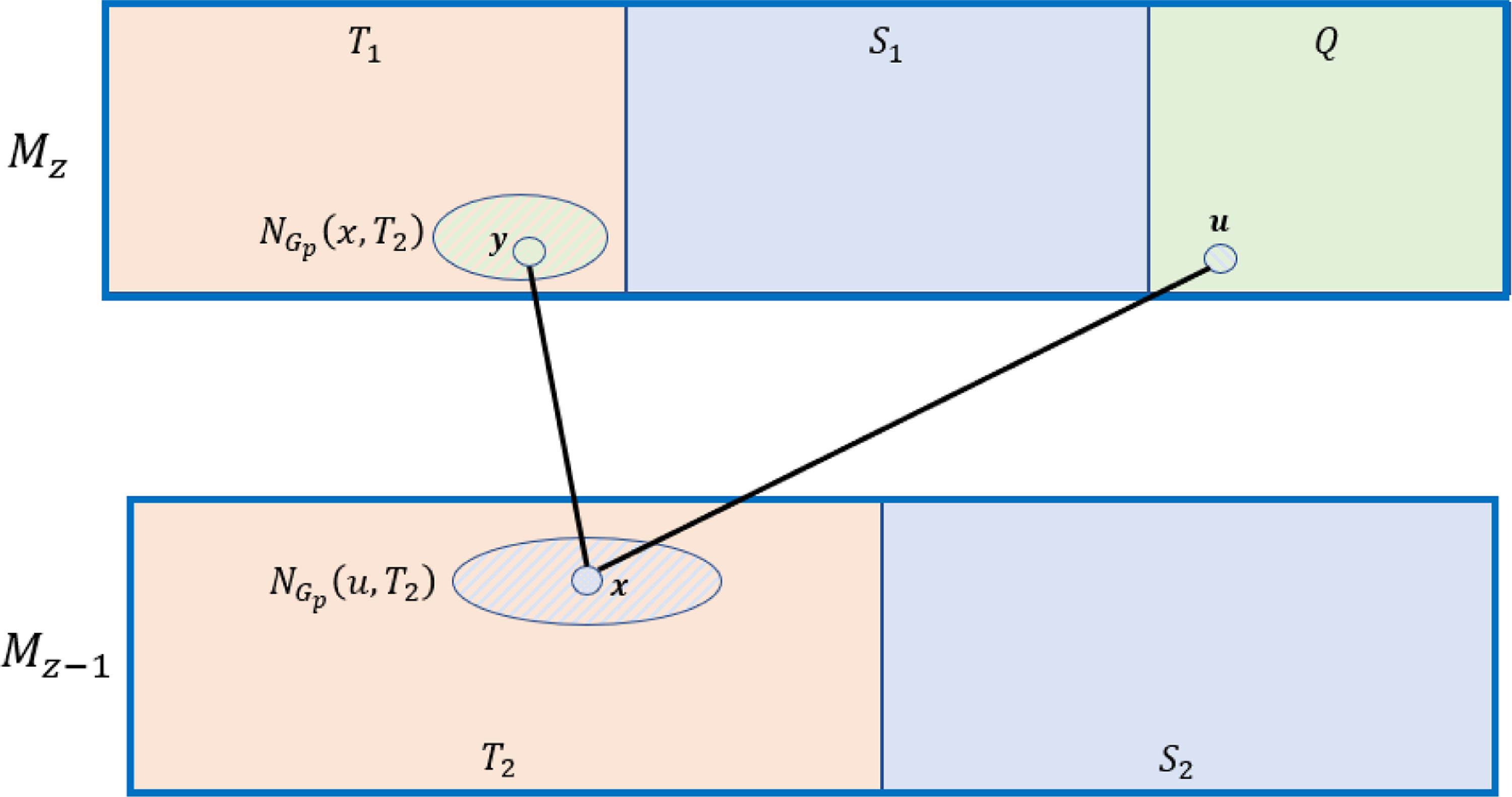
Figure 2. The vertex
 $u\in Q$
and its exposed neighbourhood in
$u\in Q$
and its exposed neighbourhood in
 $T_2$
, and a vertex
$T_2$
, and a vertex
 $x\in T_2$
and its exposed neighbourhood in
$x\in T_2$
and its exposed neighbourhood in
 $T_1$
. Note that in the course of the exploration process, all the vertices in
$T_1$
. Note that in the course of the exploration process, all the vertices in
 $N_{G_p}(x,T_2)$
move from
$N_{G_p}(x,T_2)$
move from
 $T_1$
to
$T_1$
to
 $Q$
, the vertex
$Q$
, the vertex
 $x$
(and, subsequently, all the vertices from
$x$
(and, subsequently, all the vertices from
 $N_{G_p}(u,T_2)$
) move to
$N_{G_p}(u,T_2)$
) move to
 $S_2$
, and, finally, the vertex
$S_2$
, and, finally, the vertex
 $u$
moves to
$u$
moves to
 $S_1$
.
$S_1$
.
We run the algorithm until either
 $Q$
is empty, or
$Q$
is empty, or
 $|S_1\cup S_2\cup Q|=\sqrt{t}$
. Let us first note that at all times,
$|S_1\cup S_2\cup Q|=\sqrt{t}$
. Let us first note that at all times,
 $Q\cup S_1\cup T_1\subseteq M_z$
, and
$Q\cup S_1\cup T_1\subseteq M_z$
, and
 $S_2\cup T_2\subseteq M_{z-1}$
.
$S_2\cup T_2\subseteq M_{z-1}$
.
Observe that, since at all times
 $|S_1\cup S_2\cup Q|\le \sqrt{t}$
, we have that for every
$|S_1\cup S_2\cup Q|\le \sqrt{t}$
, we have that for every
 $u\in Q$
,
$u\in Q$
,
 $d(u, T_2)\ge zs-\sqrt{t}\ge \frac{zs}{2}$
 $\left(\textrm{since}\; z\ge \frac{1+\delta }{10\sqrt{s}p}\ge \frac{(1+\delta )t}{10\sqrt{s}}\right),$
and for every
$\left(\textrm{since}\; z\ge \frac{1+\delta }{10\sqrt{s}p}\ge \frac{(1+\delta )t}{10\sqrt{s}}\right),$
and for every
 $w\in T_2$
,
$w\in T_2$
,
 $d(w, T_1)\ge t-z+1-\sqrt{t}\ge \frac{2t}{3}$
(since
$d(w, T_1)\ge t-z+1-\sqrt{t}\ge \frac{2t}{3}$
(since
 $z\le \frac{t}{\sqrt{s}}$
and
$z\le \frac{t}{\sqrt{s}}$
and
 $s$
is large enough). We can thus couple the tree
$s$
is large enough). We can thus couple the tree
 $B_1$
constructed in our truncated algorithm with a Galton-Watson tree
$B_1$
constructed in our truncated algorithm with a Galton-Watson tree
 $B_2$
rooted at
$B_2$
rooted at
 $v$
, such that for all
$v$
, such that for all
 $i$
, the offspring distribution at the
$i$
, the offspring distribution at the
 $2i$
th generation (where we start at generation
$2i$
th generation (where we start at generation
 $0$
, with
$0$
, with
 $v$
) is
$v$
) is
 $\text{Bin}\left (\frac{zs}{2},p\right )$
, and at the
$\text{Bin}\left (\frac{zs}{2},p\right )$
, and at the
 $(2i+1)$
th generation is
$(2i+1)$
th generation is
 $\text{Bin}\left (\frac{2t}{3},p\right )$
, such that
$\text{Bin}\left (\frac{2t}{3},p\right )$
, such that
 $B_2$
is isomorphic to a subgraph of
$B_2$
is isomorphic to a subgraph of
 $B_1$
as long as
$B_1$
as long as
 $|B_1|\le \sqrt{t}$
.
$|B_1|\le \sqrt{t}$
.
Let us denote by
 $Z_i$
be the number of vertices at depth
$Z_i$
be the number of vertices at depth
 $i$
in
$i$
in
 $B_2$
(where
$B_2$
(where
 $Z_0=1$
, and the vertex in the
$Z_0=1$
, and the vertex in the
 $0$
th depth is
$0$
th depth is
 $v$
). We then have by the above and by Lemma 10 that, for large enough
$v$
). We then have by the above and by Lemma 10 that, for large enough
 $s$
,
$s$
,
 \begin{align*} \mathbb{P}\left [Z_{2(i+1)}\le \frac{zs^{\frac{2}{3}}x}{10t}\mid Z_{2i}=x\right ]&\le \mathbb{P}\left [Z_{2i+1}\le \frac{zs^{\frac{2}{3}}x}{t}\mid Z_{2i}=x\right ]+\mathbb{P}\left [Z_{2(i+1)}\le \frac{zs^{\frac{2}{3}}x}{10t}\mid Z_{2i+1}\ge \frac{zs^{\frac{2}{3}}x}{t}\right ]\\[10pt] &\le \mathbb{P}\left [\text{Bin}\left (\frac{zsx}{2},p\right )\le \frac{zs^{\frac{2}{3}}x}{t}\right ]+\mathbb{P}\left [\text{Bin}\left (\frac{2zs^{\frac{2}{3}}x}{3},p\right )\le \frac{zs^{\frac{2}{3}}x}{10t}\right ]\\[5pt] &\le \exp \left (\!-\!2x\right )+ \exp \left (-\frac{3x}{16}\right )\le \exp \left (-\frac{x}{100}\right ), \end{align*}
where the penultimate inequality follows since
 $p\ge \frac{1-\epsilon }{3t}$
and
$p\ge \frac{1-\epsilon }{3t}$
and
 $zsp\ge \frac{(1+\delta )\sqrt{s}}{10}$
. Hence, we obtain:
$zsp\ge \frac{(1+\delta )\sqrt{s}}{10}$
. Hence, we obtain:
 \begin{align*} \mathbb{P}\left [\exists i \text{ such that } Z_{2i}\le \left (\frac{zs^{\frac{2}{3}}}{10t}\right )^i\right ]&\le \sum _{i=1}^{\infty }\mathbb{P}\left [Z_{2i}\le \left (\frac{zs^{\frac{2}{3}}}{10t}\right )^i \mid Z_{2(2i-1)}\ge \left (\frac{zs^{\frac{2}{3}}}{10t}\right )^{i-1}\right ]\\[5pt] &\le \sum _{i=1}^{\infty }\exp \left (-\frac{1}{100}\cdot \left (\frac{zs^{\frac{2}{3}}}{10t}\right )^i\right )\le \exp \left (-\frac{1}{200}\right ), \end{align*}
where the last inequality follows since
 $p\le \frac{1}{t}$
, and
$p\le \frac{1}{t}$
, and
 $z\ge \frac{(1+\delta )}{10\sqrt{s}p}\ge \frac{(1+\delta )t}{10\sqrt{s}}$
, and we take
$z\ge \frac{(1+\delta )}{10\sqrt{s}p}\ge \frac{(1+\delta )t}{10\sqrt{s}}$
, and we take
 $s$
to be large enough. In particular,
$s$
to be large enough. In particular,
 $\frac{zs^{\frac{2}{3}}}{10t}\gt 1$
, and hence the Galton-Watson tree grows to infinity with probability at least
$\frac{zs^{\frac{2}{3}}}{10t}\gt 1$
, and hence the Galton-Watson tree grows to infinity with probability at least
 $\exp \left (-\frac{1}{200}\right )$
, and therefore with probability at least
$\exp \left (-\frac{1}{200}\right )$
, and therefore with probability at least
 $\exp \left (-\frac{1}{200}\right )$
we have that
$\exp \left (-\frac{1}{200}\right )$
we have that
 $|B_2|=\sqrt{t}$
and hence
$|B_2|=\sqrt{t}$
and hence
 $|S_1\cup S_2\cup Q|=\sqrt{t}$
at some point. We thus have that with the same probability, we have a connected set
$|S_1\cup S_2\cup Q|=\sqrt{t}$
at some point. We thus have that with the same probability, we have a connected set
 $W$
such that
$W$
such that
 $v\in W$
,
$v\in W$
,
 $W$
is connected in
$W$
is connected in
 $G_p$
, and
$G_p$
, and
 $|W|=\sqrt{t}$
. Let us argue further that, in fact,
$|W|=\sqrt{t}$
. Let us argue further that, in fact,
 $|W\cap \left (S_1\cup Q\right )|\ge \frac{\sqrt{t}}{22}$
. Consider any vertex
$|W\cap \left (S_1\cup Q\right )|\ge \frac{\sqrt{t}}{22}$
. Consider any vertex
 $w\in S_2$
. Crucially, observe that by the construction of the exploration process, unless
$w\in S_2$
. Crucially, observe that by the construction of the exploration process, unless
 $w$
is the last vertex we have moved such that now
$w$
is the last vertex we have moved such that now
 $|B_1|=\sqrt{t}$
, after we move
$|B_1|=\sqrt{t}$
, after we move
 $w$
from
$w$
from
 $T_2$
to
$T_2$
to
 $S_2$
we expose the neighbourhood of
$S_2$
we expose the neighbourhood of
 $w$
in
$w$
in
 $T_1$
(see Figure 2). If
$T_1$
(see Figure 2). If
 $|N_{G_p}(w, T_1)|\ge 1$
, then we added at least one child of
$|N_{G_p}(w, T_1)|\ge 1$
, then we added at least one child of
 $w$
to
$w$
to
 $B_1$
. The probability that
$B_1$
. The probability that
 $|N_{G_p}(w,T_1)|=0$
is at most
$|N_{G_p}(w,T_1)|=0$
is at most
 \begin{align*} (1-p)^{\frac{2t}{3}-\sqrt{t}}\le \left (1-\frac{1-\epsilon }{3t}\right )^{\frac{t}{2}}\le \exp \left (-\frac{1-\epsilon }{6}\right )\le \frac{9}{10}. \end{align*}
Hence the number of
 $w\in S_2$
which does not have at least one child, stochastically dominates
$w\in S_2$
which does not have at least one child, stochastically dominates
 $1+\text{Bin}\left (\sqrt{t},\frac{9}{10}\right )$
(where we use the fact that
$1+\text{Bin}\left (\sqrt{t},\frac{9}{10}\right )$
(where we use the fact that
 $|B_1|\le \sqrt{t}$
and our stochastic domination on the number of neighbours). Hence, by Lemma 11, the number of vertices
$|B_1|\le \sqrt{t}$
and our stochastic domination on the number of neighbours). Hence, by Lemma 11, the number of vertices
 $w\in T_2$
which do not have at least one child in
$w\in T_2$
which do not have at least one child in
 $T_1$
in
$T_1$
in
 $B_1$
(that afterwards moves to
$B_1$
(that afterwards moves to
 $Q_1$
and perhaps subsequently to
$Q_1$
and perhaps subsequently to
 $S_1$
) is whp at most
$S_1$
) is whp at most
 $\frac{10\sqrt{t}}{11}$
. Therefore, there are at most
$\frac{10\sqrt{t}}{11}$
. Therefore, there are at most
 $\frac{10\sqrt{t}}{11}$
vertices in
$\frac{10\sqrt{t}}{11}$
vertices in
 $S_2$
which do not have a child in
$S_2$
which do not have a child in
 $B_1$
. Since
$B_1$
. Since
 $B_1$
is a tree, these children are distinct for distinct
$B_1$
is a tree, these children are distinct for distinct
 $w$
, and they all lie in
$w$
, and they all lie in
 $S_1$
or
$S_1$
or
 $Q$
. It follows that whp
$Q$
. It follows that whp
 $|S_1\cup Q|\ge |S_2|-\frac{10\sqrt{t}}{11}$
, and hence with probability at least
$|S_1\cup Q|\ge |S_2|-\frac{10\sqrt{t}}{11}$
, and hence with probability at least
 $c\gt 0$
, we have that
$c\gt 0$
, we have that
 $|S_1\cup Q|\ge \frac{\sqrt{t}}{22}$
, and hence
$|S_1\cup Q|\ge \frac{\sqrt{t}}{22}$
, and hence
 $|W\cap M_{z}|\ge \frac{\sqrt{t}}{22}$
, completing the case of
$|W\cap M_{z}|\ge \frac{\sqrt{t}}{22}$
, completing the case of
 $k=1$
.
$k=1$
.
We proceed in a manner somewhat similar to the proof of Lemma 16. Let
 $k\ge 2$
and assume the statement holds with
$k\ge 2$
and assume the statement holds with
 $c_1(z', k-1,\epsilon ',\delta ')$
and
$c_1(z', k-1,\epsilon ',\delta ')$
and
 $c_2(z', k-1,\epsilon ',\delta ')$
for all relevant values of
$c_2(z', k-1,\epsilon ',\delta ')$
for all relevant values of
 $z'$
,
$z'$
,
 $\epsilon '$
and
$\epsilon '$
and
 $\delta '$
. We argue via a two-stage exposure, with
$\delta '$
. We argue via a two-stage exposure, with
 $p_2=\frac{1}{t\log t}$
and
$p_2=\frac{1}{t\log t}$
and
 $p_1=\frac{p-p_2}{1-p_2}$
so that
$p_1=\frac{p-p_2}{1-p_2}$
so that
 $(1-p_1)(1-p_2)=1-p$
. Note that
$(1-p_1)(1-p_2)=1-p$
. Note that
 $G_p$
has the same distribution as
$G_p$
has the same distribution as
 $G_{p_1}\cup G_{p_2}$
, and that
$G_{p_1}\cup G_{p_2}$
, and that
 $p_1\ge (1-o_t(1))p\ge \frac{1-\epsilon _1}{3t}$
for some
$p_1\ge (1-o_t(1))p\ge \frac{1-\epsilon _1}{3t}$
for some
 $\epsilon _1\gt 0$
constant. Similarly,
$\epsilon _1\gt 0$
constant. Similarly,
 $z\ge \frac{1+\delta }{10\sqrt{s}p}\ge \frac{1+\delta _1}{10\sqrt{s}p_1}$
, and we can thus begin in the same manner as
$z\ge \frac{1+\delta }{10\sqrt{s}p}\ge \frac{1+\delta _1}{10\sqrt{s}p_1}$
, and we can thus begin in the same manner as
 $k=1$
, and find with probability at least
$k=1$
, and find with probability at least
 $c\gt 0$
, a set
$c\gt 0$
, a set
 $W_0$
such that
$W_0$
such that
 $v\in W_0$
,
$v\in W_0$
,
 $W_0$
is connected in
$W_0$
is connected in
 $G_p$
,
$G_p$
,
 $|W_0|=\sqrt{t}$
and
$|W_0|=\sqrt{t}$
and
 $|W_0\cap M_z|\ge \frac{\sqrt{t}}{22}$
. We further note that
$|W_0\cap M_z|\ge \frac{\sqrt{t}}{22}$
. We further note that
 $W_0\subseteq V(\Gamma )$
. We proceed under the assumption that indeed
$W_0\subseteq V(\Gamma )$
. We proceed under the assumption that indeed
 $|W_0|=\sqrt{t}$
. Let us enumerate the vertices in
$|W_0|=\sqrt{t}$
. Let us enumerate the vertices in
 $W_0\cap M_z$
as
$W_0\cap M_z$
as
 $\left \{v_1,\ldots,v_{\ell }\right \}$
, where
$\left \{v_1,\ldots,v_{\ell }\right \}$
, where
 $\ell \ge \frac{\sqrt{t}}{22}$
and
$\ell \ge \frac{\sqrt{t}}{22}$
and
 $\ell \le \sqrt{t}$
(since
$\ell \le \sqrt{t}$
(since
 $|W_0|=\sqrt{t}$
).
$|W_0|=\sqrt{t}$
).
Using Lemma 13, we can find pairwise disjoint projections
 $H_1,\ldots, H_{\ell }$
of
$H_1,\ldots, H_{\ell }$
of
 $G$
, each having dimension at least
$G$
, each having dimension at least
 $t-\sqrt{t}$
, such that each
$t-\sqrt{t}$
, such that each
 $v_i\in W_0$
is in exactly one of
$v_i\in W_0$
is in exactly one of
 $H_i$
’s.
$H_i$
’s.
We now intend to find pairwise disjoint projection of
 $G$
, each with a vertex in
$G$
, each with a vertex in
 $M_{z}$
, to which we can apply our induction hypothesis. Note that, in an arbitrary projection
$M_{z}$
, to which we can apply our induction hypothesis. Note that, in an arbitrary projection
 $H'$
of
$H'$
of
 $G$
with dimension
$G$
with dimension
 $t'$
, the set
$t'$
, the set
 $M_z \cap V(H')$
will still be a layer of
$M_z \cap V(H')$
will still be a layer of
 $H'$
. However, for the vertices in this layer, the number of ‘active’ coordinates in
$H'$
. However, for the vertices in this layer, the number of ‘active’ coordinates in
 $H'$
which are centres of stars will be some number between
$H'$
which are centres of stars will be some number between
 $z$
and
$z$
and
 $z-(t-t')$
. Our approach here is then almost identical to that of the proof of Lemma 16, with the slight difference that we want our vertices to be in
$z-(t-t')$
. Our approach here is then almost identical to that of the proof of Lemma 16, with the slight difference that we want our vertices to be in
 $M_{z}$
, and have
$M_{z}$
, and have
 $z'$
centre coordinates inside the projected subgraph, for some
$z'$
centre coordinates inside the projected subgraph, for some
 $z'$
such that
$z'$
such that
 $z'\ge \frac{1+\delta '}{10\sqrt{s}p_1}$
for some
$z'\ge \frac{1+\delta '}{10\sqrt{s}p_1}$
for some
 $\delta '\gt 0$
.
$\delta '\gt 0$
.
In order to obtain that, we begin by exposing some carefully chosen sets of edges with probability
 $p_2$
. Observe that for each
$p_2$
. Observe that for each
 $v_i\in W_0\cap M_{z}$
, we have that
$v_i\in W_0\cap M_{z}$
, we have that
 \begin{equation*} |N_{H_i\cap \Gamma }(v_i)|\ge |N_\Gamma (v_i)|-s\cdot \sqrt {t}\ge \frac {zs}{3}, \end{equation*}
where the first inequality follows since the dimension of
 $H_i$
is at least
$H_i$
is at least
 $t-\sqrt{t}$
and the maximum degree of the base graphs is
$t-\sqrt{t}$
and the maximum degree of the base graphs is
 $s$
. We further note that
$s$
. We further note that
 $N_{H_i\cap \Gamma }(v_i)\subseteq M_{z-1}$
. Let
$N_{H_i\cap \Gamma }(v_i)\subseteq M_{z-1}$
. Let
 \begin{equation*} W_1=\bigcup _{i\in \left [\sqrt {\ell }\right ]}N_{H_i\cap \Gamma }(v_i)\subseteq M_{z-1}. \end{equation*}
Then, recalling that the
 $H_i$
’s are pairwise disjoint, we have that
$H_i$
’s are pairwise disjoint, we have that
 \begin{align*} |W_1|\ge \frac{\sqrt{t}}{25}\cdot \frac{zs}{3}\ge \frac{\sqrt{t}(1+\delta )\sqrt{s}}{750p}\ge t^{\frac{3}{2}}, \end{align*}
where we used our assumption that
 $z\ge \frac{1+\delta }{10\sqrt{s}p}$
and that
$z\ge \frac{1+\delta }{10\sqrt{s}p}$
and that
 $s$
is large enough.
$s$
is large enough.
We now expose the edges between
 $W_0$
and
$W_0$
and
 $W_1$
in
$W_1$
in
 $G_{p_2}$
. Let us denote the set of vertices in
$G_{p_2}$
. Let us denote the set of vertices in
 $W_1$
that are connected with
$W_1$
that are connected with
 $W_0$
in
$W_0$
in
 $G_{p_2}$
by
$G_{p_2}$
by
 $W_1'$
. Then,
$W_1'$
. Then,
 $|W_1'|$
stochastically dominates
$|W_1'|$
stochastically dominates
 $\text{Bin}\left (t^{\frac{3}{2}},p_2\right )$
. Thus, by Lemma 10, we have that whp
$\text{Bin}\left (t^{\frac{3}{2}},p_2\right )$
. Thus, by Lemma 10, we have that whp
 $|W_1'|\ge \frac{\sqrt{t}}{10\log t}$
. We assume in what follows that this property holds.
$|W_1'|\ge \frac{\sqrt{t}}{10\log t}$
. We assume in what follows that this property holds.
We now expose the edges in
 $G_{p_2}$
between
$G_{p_2}$
between
 $W_1'$
and
$W_1'$
and
 $M_{z}\setminus W_0$
, recalling that by our assumption
$M_{z}\setminus W_0$
, recalling that by our assumption
 $|W_0|=\sqrt{t}$
. Note that for every
$|W_0|=\sqrt{t}$
. Note that for every
 $w_i\in W_1'$
, we have that
$w_i\in W_1'$
, we have that
 \begin{equation*}|N_{H_i\cap \Gamma }(w_i) \cap (M_{z}\setminus W_0)|\ge |N_\Gamma (w_1)|-2s\cdot \sqrt {t}\ge \frac {t}{3},\end{equation*}
and
 $N_{H_i\cap \Gamma }(w_i) \cap (M_{z}\setminus W_0) \subseteq M_{z}$
. Let
$N_{H_i\cap \Gamma }(w_i) \cap (M_{z}\setminus W_0) \subseteq M_{z}$
. Let
 \begin{equation*} W_2=\bigcup _{i\in \left [\ell \right ]} N_{H_i\cap \Gamma }(w_i)\cap (M_{z}\setminus W_0)\subseteq M_{z}, \end{equation*}
where we note that by the projection Lemma (lemma 13) and our construction, these neighbourhoods are disjoint. Then whp
 $|W_2|\ge \frac{t}{3}\cdot \frac{\sqrt{t}}{10\log t}.$
Let
 $W_2'\subseteq M_{z}$
be the set of vertices in
$W_2'\subseteq M_{z}$
be the set of vertices in
 $W_2$
that are connected with
$W_2$
that are connected with
 $W_1'$
in
$W_1'$
in
 $G_{p_2}$
. Then,
$G_{p_2}$
. Then,
 $|W_2'|$
stochastically dominates
$|W_2'|$
stochastically dominates
 $\text{Bin}\left (\frac{t^{\frac{3}{2}}}{10\log t},p_2\right ).$
Thus, by Lemma 10, we have that whp
$\text{Bin}\left (\frac{t^{\frac{3}{2}}}{10\log t},p_2\right ).$
Thus, by Lemma 10, we have that whp
 $|W_2'|\ge \frac{\sqrt{t}}{20\log ^2t}$
and
$|W_2'|\ge \frac{\sqrt{t}}{20\log ^2t}$
and
 $|W_2'|\le \sqrt{t}$
. We assume henceforth that these two properties hold.
$|W_2'|\le \sqrt{t}$
. We assume henceforth that these two properties hold.
The subsequent part of the proof is almost identical to that of the proof of Lemma 16, where here we only need to run the inductive step constantly many times (as opposed to
 $\omega (1)$
times), allowing us to analyse it in a more straightforward manner.
$\omega (1)$
times), allowing us to analyse it in a more straightforward manner.
Indeed, let
 $W_{2,i}'=W_2'\cap V(H_i)\subseteq M_{z}$
. We thus have now our set of vertices in
$W_{2,i}'=W_2'\cap V(H_i)\subseteq M_{z}$
. We thus have now our set of vertices in
 $M_{z}$
. Now, for each
$M_{z}$
. Now, for each
 $i$
, we apply once again Lemma 13 to find a family of
$i$
, we apply once again Lemma 13 to find a family of
 $|W_{2,i}'|\;:\!=\; \ell _i\le \sqrt{t}$
pairwise disjoint projections of
$|W_{2,i}'|\;:\!=\; \ell _i\le \sqrt{t}$
pairwise disjoint projections of
 $H_i$
, which we denote by
$H_i$
, which we denote by
 $H_{i,1},\ldots, H_{i,\ell _i}$
, such that every vertex of
$H_{i,1},\ldots, H_{i,\ell _i}$
, such that every vertex of
 $W_{2,i}'\subseteq M_{z}$
is in exactly one of the
$W_{2,i}'\subseteq M_{z}$
is in exactly one of the
 $H_{i,j}$
, and each of the
$H_{i,j}$
, and each of the
 $H_{i,j}$
is of dimension at least
$H_{i,j}$
is of dimension at least
 $t-2\sqrt{t}$
. We have that for all
$t-2\sqrt{t}$
. We have that for all
 $i,j$
, the number of centre coordinates of
$i,j$
, the number of centre coordinates of
 $v_{i,j}$
in
$v_{i,j}$
in
 $H_{i,j}$
, denote it by
$H_{i,j}$
, denote it by
 $z_{i,j}$
, is at least
$z_{i,j}$
, is at least
 $z-2s\sqrt{t}$
. Recall that
$z-2s\sqrt{t}$
. Recall that
 $p_1\ge \frac{1-\epsilon _1}{3t}$
, and note that
$p_1\ge \frac{1-\epsilon _1}{3t}$
, and note that
 \begin{align*} z_{i,j} \ge z-2s\sqrt{t}\ge \frac{1+\delta }{10\sqrt{s}p}-2s\sqrt{t} \ge \frac{1+\delta _2}{10\sqrt{s}p} \ge \frac{1+\delta _3}{10\sqrt{s}p_1} \end{align*}
for some
 $\delta _2,\delta _3\gt 0$
, where we used
$\delta _2,\delta _3\gt 0$
, where we used
 $p\le \frac{1}{t}$
and
$p\le \frac{1}{t}$
and
 $p_1=(1-o(1))p$
. Altogether, the
$p_1=(1-o(1))p$
. Altogether, the
 $v_{i,j}$
(that is, their corresponding
$v_{i,j}$
(that is, their corresponding
 $z_{i,j}$
) together with
$z_{i,j}$
) together with
 $p_1$
satisfy the conditions of the induction hypothesis for some
$p_1$
satisfy the conditions of the induction hypothesis for some
 $\epsilon _{i,j},\delta _{i,j}\gt 0$
.
$\epsilon _{i,j},\delta _{i,j}\gt 0$
.
As in the proof of Lemma 16, note that when we ran the algorithm on
 $G_{p_1}$
, we did not query any of the edges inside any of the
$G_{p_1}$
, we did not query any of the edges inside any of the
 $H_{i,j}$
. By the above inequality we can apply the induction hypothesis to
$H_{i,j}$
. By the above inequality we can apply the induction hypothesis to
 $v_{i,j}$
in
$v_{i,j}$
in
 $G_{p_1}\cap H_{i,j}$
and conclude that with probability at least
$G_{p_1}\cap H_{i,j}$
and conclude that with probability at least
 $c_1(z_{i,j},k-1,\epsilon _{i,j},\delta _{i,j})$
, there exists a connected set
$c_1(z_{i,j},k-1,\epsilon _{i,j},\delta _{i,j})$
, there exists a connected set
 $W_{i,j}$
such that
$W_{i,j}$
such that
 $v_{i,j}$
is
$v_{i,j}$
is
 $W_{i,j}$
,
$W_{i,j}$
,
 $|W_{i,j}\cap M_{z}|\ge c_2(z_{i,j},k-1,\epsilon _{i,j},\delta _{i,j})t^{\frac{k-1}{6}}$
. Let
$|W_{i,j}\cap M_{z}|\ge c_2(z_{i,j},k-1,\epsilon _{i,j},\delta _{i,j})t^{\frac{k-1}{6}}$
. Let
 $c'_1=\min _{i,j}c_1(z_{i,j},k-1,\epsilon _{i,j},\delta _{i,j})$
and
$c'_1=\min _{i,j}c_1(z_{i,j},k-1,\epsilon _{i,j},\delta _{i,j})$
and
 $c'_{\!\!2}=\min _{i,j}c_2(z_{i,j},k-1,\epsilon _{i,j},\delta _{i,j})$
. Noting that the above described events are independent for every
$c'_{\!\!2}=\min _{i,j}c_2(z_{i,j},k-1,\epsilon _{i,j},\delta _{i,j})$
. Noting that the above described events are independent for every
 $H_{i,j}$
, we obtain by Lemma 10 that whp, at least
$H_{i,j}$
, we obtain by Lemma 10 that whp, at least
 $\frac{c'_1\sqrt{t}}{40\log ^2t}$
of the
$\frac{c'_1\sqrt{t}}{40\log ^2t}$
of the
 $H_{i,j}$
have that
$H_{i,j}$
have that
 $|W_{i,j}\cap M_{z}|\ge c'_{\!\!2}t^{\frac{k-1}{6}}$
. Thus, with probability at least
$|W_{i,j}\cap M_{z}|\ge c'_{\!\!2}t^{\frac{k-1}{6}}$
. Thus, with probability at least
 $c'_1+o(1)\;:\!=\; c_1$
, we have found a connected set
$c'_1+o(1)\;:\!=\; c_1$
, we have found a connected set
 $W$
such that
$W$
such that
 $v$
is in
$v$
is in
 $W$
, and there is some
$W$
, and there is some
 $c_2\gt 0$
such that
$c_2\gt 0$
such that
 \begin{align*} |W\cap M_{z}|\ge \frac{c'_{\!\!1}\sqrt{t}}{40\log ^2t}\cdot c'_{\!\!2}t^{\frac{k-1}{6}}\gt c_2t^{\frac{k}{6}}, \end{align*}
completing the induction step.
We now turn to show that whp many of the vertices with
 $z\;:\!=\; \frac{t}{\sqrt{s}}$
centre coordinates are contained in big connected sets in
$z\;:\!=\; \frac{t}{\sqrt{s}}$
centre coordinates are contained in big connected sets in
 $G_p$
.
$G_p$
.
Lemma 20.
Let
 $s$
be a large enough integer. Let
$s$
be a large enough integer. Let
 $p\ge \frac{1}{3t}$
and let
$p\ge \frac{1}{3t}$
and let
 $k\gt 0$
be an integer. Let
$k\gt 0$
be an integer. Let
 $z\;:\!=\; \frac{t}{\sqrt{s}}$
. Let
$z\;:\!=\; \frac{t}{\sqrt{s}}$
. Let
 $M_{z}$
be the set of vertices with
$M_{z}$
be the set of vertices with
 $z$
centre coordinates in
$z$
centre coordinates in
 $G$
and let
$G$
and let
 $W\subseteq M_{z}$
be the set of vertices in
$W\subseteq M_{z}$
be the set of vertices in
 $M_{z}$
that belong to components with at least
$M_{z}$
that belong to components with at least
 $t^k$
vertices in
$t^k$
vertices in
 $M_{z}$
in
$M_{z}$
in
 $G_p$
. Then, there exists a constant
$G_p$
. Then, there exists a constant
 $\rho \gt 0$
such that
whp
,
$\rho \gt 0$
such that
whp
,
 \begin{align*} |W|\ge \rho |M_{z}|\ge |G|^{1-s^{-\frac{1}{5}}}. \end{align*}
Proof. Observe that in order to choose a vertex in
 $M_{z}$
we have
$M_{z}$
we have
 $\binom{t}{z}$
choices for the
$\binom{t}{z}$
choices for the
 $z$
-set of coordinates which are the centre of a star, and then we have
$z$
-set of coordinates which are the centre of a star, and then we have
 $s^{t-z}$
choices for the leaf coordinates. It follows that
$s^{t-z}$
choices for the leaf coordinates. It follows that
 \begin{align*} |M_{z}|= \binom{t}{z}s^{t-z}\ge \left (\sqrt{s}\right )^{\frac{t}{\sqrt{s}}}s^{\left (1-\frac{1}{\sqrt{s}}\right )t} \ge (s+1)^{\left (1-s^{-\frac{1}{3}}\right )t} = |G|^{1-s^{-\frac{1}{3}}}, \end{align*}
where the penultimate inequality holds for any
 $s$
large enough.
$s$
large enough.
By Lemma 19, there is some constant
 $c' \gt 0$
such that every
$c' \gt 0$
such that every
 $v\in M_{z}$
belongs to a connected set of order
$v\in M_{z}$
belongs to a connected set of order
 $t^k$
with probability at least
$t^k$
with probability at least
 $c'\gt 0$
. We thus have that
$c'\gt 0$
. We thus have that
 \begin{equation*} \mathbb {E}[|W|]\ge c'|M_{z}|\ge c'|G|^{1-s^{-\frac {1}{3}}}. \end{equation*}
Consider the edge-exposure martingale on
 $G_p$
. It has length
$G_p$
. It has length
 $|E(G)| = \frac{st}{s+1} |G| \leq 2t |G|$
, and the addition or deletion of an edge can change the value of
$|E(G)| = \frac{st}{s+1} |G| \leq 2t |G|$
, and the addition or deletion of an edge can change the value of
 $|W|$
by at most
$|W|$
by at most
 $2t^k$
. Therefore, by Lemma 11, we have for
$2t^k$
. Therefore, by Lemma 11, we have for
 $\rho =\frac{c'}{2}\gt 0$
that
$\rho =\frac{c'}{2}\gt 0$
that
 \begin{align*} \mathbb{P}\left [|W|\le \rho |M_{z}|\right ]&\le \mathbb{P}\left [|W|\le \frac{\mathbb{E}|W|}{2}\right ] \le 2\exp \left (-\frac{|G|^{2-2s^{-\frac{1}{3}}}}{16|G|t^{2k+1}} \right ) \le 2\exp \left (-|G|^{1-s^{-\frac{1}{4}}}\right )=o(1), \end{align*}
as long as
 $s$
is large enough. It follows that whp
$s$
is large enough. It follows that whp
 \begin{equation*} |W|\ge \rho |M_{z}|\ge \frac {c'}{2}|G|^{1-s^{-\frac {1}{4}}} \geq |G|^{1-s^{-\frac {1}{5}}}. \end{equation*}
We note that while
 $M_z$
, where
$M_z$
, where
 $z=\frac{t}{\sqrt{s}}$
, takes a polynomial fraction of the vertices, this set of vertices still only amounts to
$z=\frac{t}{\sqrt{s}}$
, takes a polynomial fraction of the vertices, this set of vertices still only amounts to
 $o(|G|)$
. Thus, we cannot use global isoperimetric properties of
$o(|G|)$
. Thus, we cannot use global isoperimetric properties of
 $G$
to find typically sufficiently many short paths between relevant (respecting) partitions of
$G$
to find typically sufficiently many short paths between relevant (respecting) partitions of
 $M_z$
, as we do in the proof of Theorem 8. Instead, we need to look at local isoperimetric properties of
$M_z$
, as we do in the proof of Theorem 8. Instead, we need to look at local isoperimetric properties of
 $M_z$
, such as the isoperimetric property of its two-neighbourhood in
$M_z$
, such as the isoperimetric property of its two-neighbourhood in
 $G$
, in order to show that whp many of the large connected sets in
$G$
, in order to show that whp many of the large connected sets in
 $G_p\cap M_z$
in fact belong to the same connected component in
$G_p\cap M_z$
in fact belong to the same connected component in
 $G_p$
.
$G_p$
.
Proof of Theorem 9. Assume that all the conditions in Theorem 9 hold.
Once again, we argue via a two-round exposure. Let
 $\epsilon$
be a small enough constant, such that
$\epsilon$
be a small enough constant, such that
 $p_2=\frac{\epsilon }{3t}$
,
$p_2=\frac{\epsilon }{3t}$
,
 $p_1=\frac{1}{3t}$
and
$p_1=\frac{1}{3t}$
and
 $(1-p_1)(1-p_2)=1-p$
, noting that
$(1-p_1)(1-p_2)=1-p$
, noting that
 $G_{p_1} \cup G_{p_2}$
has the same distribution as
$G_{p_1} \cup G_{p_2}$
has the same distribution as
 $G_p$
.
$G_p$
.
Let
 $z\;:\!=\; \frac{t}{\sqrt{s}}$
. Let
$z\;:\!=\; \frac{t}{\sqrt{s}}$
. Let
 $M_{z}$
be the set of vertices with
$M_{z}$
be the set of vertices with
 $z$
centre coordinates in
$z$
centre coordinates in
 $G$
, and let
$G$
, and let
 $W\subseteq M_{z}$
be the set of vertices in
$W\subseteq M_{z}$
be the set of vertices in
 $M_{z}$
belonging to a component with at least
$M_{z}$
belonging to a component with at least
 $t^{15}$
vertices in
$t^{15}$
vertices in
 $M_{z}$
in
$M_{z}$
in
 $G_{p_1}$
. Then, by Lemma 20 with
$G_{p_1}$
. Then, by Lemma 20 with
 $k=15$
, we have that there exists a constant
$k=15$
, we have that there exists a constant
 $\rho \gt 0$
such that whp,
$\rho \gt 0$
such that whp,
 \begin{align} |W|\ge \rho |M_{z}|\ge |G|^{1-s^{-\frac{1}{5}}}. \end{align}
We note further that, since the average degree
 $t = \Theta (\log |G|)$
, by a similar argument as in Lemma 17 applied to the vertices with
$t = \Theta (\log |G|)$
, by a similar argument as in Lemma 17 applied to the vertices with
 $z$
centre coordinates in
$z$
centre coordinates in
 $G$
, we claim that whp
$G$
, we claim that whp
 \begin{align} \text{every vertex in $M_{z}$ is at distance at most 2 from $W$.} \end{align}
To see why, observe that given a vertex
 $v\in M_{z}$
, we can form
$v\in M_{z}$
, we can form
 $t^{\frac{4}{3}}$
pairwise disjoint projections of
$t^{\frac{4}{3}}$
pairwise disjoint projections of
 $G$
, each isomorphic to the product of
$G$
, each isomorphic to the product of
 $(1-o(1))t$
copies of
$(1-o(1))t$
copies of
 $S(1,s)$
and each containing a vertex with
$S(1,s)$
and each containing a vertex with
 $z$
centre coordinates at distance
$z$
centre coordinates at distance
 $2$
from
$2$
from
 $v$
. Indeed, since the number
$v$
. Indeed, since the number
 $z$
of coordinates of
$z$
of coordinates of
 $v$
which are the centre of star satisfies
$v$
which are the centre of star satisfies
 $t^{\frac{2}{3}} \leq z \leq t-t^{\frac{2}{3}}$
, we can assume without loss of generality that the first
$t^{\frac{2}{3}} \leq z \leq t-t^{\frac{2}{3}}$
, we can assume without loss of generality that the first
 $t^{\frac{2}{3}}$
coordinates of
$t^{\frac{2}{3}}$
coordinates of
 $v$
are the centres of stars, and the second
$v$
are the centres of stars, and the second
 $t^{\frac{2}{3}}$
coordinates are leaves.
$t^{\frac{2}{3}}$
coordinates are leaves.
Given a pair of coordinates
 $1 \leq i \leq t^{\frac{2}{3}} \lt j \leq 2t^{\frac{2}{3}}$
, let
$1 \leq i \leq t^{\frac{2}{3}} \lt j \leq 2t^{\frac{2}{3}}$
, let
 $H_{i,j}$
be the projection of
$H_{i,j}$
be the projection of
 $G$
to the first
$G$
to the first
 $2t^{\frac{2}{3}}$
coordinates where the first
$2t^{\frac{2}{3}}$
coordinates where the first
 $2t^{\frac{2}{3}}$
coordinates agree with
$2t^{\frac{2}{3}}$
coordinates agree with
 $v$
, except that the
$v$
, except that the
 $i$
th coordinate is some arbitrary leaf and the
$i$
th coordinate is some arbitrary leaf and the
 $j$
th coordinate is the centre of the star.
$j$
th coordinate is the centre of the star.
Then, the graphs
 $H_{i,j}$
form a collection of
$H_{i,j}$
form a collection of
 $t^{\frac{4}{3}}$
pairwise disjoint projections of
$t^{\frac{4}{3}}$
pairwise disjoint projections of
 $G$
, each isomorphic to the product of
$G$
, each isomorphic to the product of
 $(1-o(1))t$
copies of
$(1-o(1))t$
copies of
 $S(1,s)$
and each containing a vertex with
$S(1,s)$
and each containing a vertex with
 $z$
centre coordinates in
$z$
centre coordinates in
 $G$
at distance
$G$
at distance
 $2$
from
$2$
from
 $v$
.
$v$
.
Since
 $p$
will still be ‘supercritical’ at these vertices in each
$p$
will still be ‘supercritical’ at these vertices in each
 $H_{i,j}$
, an argument as in Lemma 17 will imply that the expected number of vertices in
$H_{i,j}$
, an argument as in Lemma 17 will imply that the expected number of vertices in
 $M_{z}$
which are not at distance at most 2 from a vertex in
$M_{z}$
which are not at distance at most 2 from a vertex in
 $W$
is at most
$W$
is at most
 $\exp \left ( - \Omega \left (t^{\frac{4}{3}} \right )\right )|G| = o(1)$
, and so the claim follows by Markov’s inequality. We assume in the following that claim (12) holds.
$\exp \left ( - \Omega \left (t^{\frac{4}{3}} \right )\right )|G| = o(1)$
, and so the claim follows by Markov’s inequality. We assume in the following that claim (12) holds.
Let
 $A\cup B$
be a
$A\cup B$
be a
 $G_{p_1}$
-respecting partition of
$G_{p_1}$
-respecting partition of
 $W$
into two parts,
$W$
into two parts,
 $A$
and
$A$
and
 $B$
, such that
$B$
, such that
 $|A|\le |B|$
and
$|A|\le |B|$
and
 $|A|\ge \frac{|W|}{3}$
. Let
$|A|\ge \frac{|W|}{3}$
. Let
 $A'$
be the set of vertices in
$A'$
be the set of vertices in
 $A$
together with all vertices in
$A$
together with all vertices in
 $M_{z}\setminus B$
that are within distance
$M_{z}\setminus B$
that are within distance
 $2$
to
$2$
to
 $A$
, and let
$A$
, and let
 $B'$
be the set of vertices in
$B'$
be the set of vertices in
 $B$
together with all vertices in
$B$
together with all vertices in
 $M_{z}\setminus A'$
that are within distance
$M_{z}\setminus A'$
that are within distance
 $2$
to
$2$
to
 $B$
, so that
$B$
, so that
 $M_{z} = A' \cup B'$
. We require the following claim, whose proof we defer to the end of this proof:
$M_{z} = A' \cup B'$
. We require the following claim, whose proof we defer to the end of this proof:
Claim 21.
Whp
, there are at least
 $\frac{|W|}{t^{2}}$
paths of length
$\frac{|W|}{t^{2}}$
paths of length
 $2$
in
$2$
in
 $G$
between
$G$
between
 $A'$
and
$A'$
and
 $B'$
.
$B'$
.
We can extend these paths to a family of
 $A-B$
paths of length at most
$A-B$
paths of length at most
 $6$
(see Figure 3) and then, very crudely, since
$6$
(see Figure 3) and then, very crudely, since
 $\Delta (G)=st$
, we can greedily thin this family to a set of
$\Delta (G)=st$
, we can greedily thin this family to a set of
 $\frac{|W|}{36s^6t^{8}}$
edge-disjoint
$\frac{|W|}{36s^6t^{8}}$
edge-disjoint
 $A-B$
paths of length at most
$A-B$
paths of length at most
 $6$
.
$6$
.

Figure 3. An extension of a partition
 $A\cup B$
of
$A\cup B$
of
 $W$
to a partition
$W$
to a partition
 $A'\cup B'$
of
$A'\cup B'$
of
 $M_{z}$
. Each
$M_{z}$
. Each
 $A'-B'$
two-path (solid) can be extended into an
$A'-B'$
two-path (solid) can be extended into an
 $A-B$
six-path (solid and dashed). Note that some vertices in these paths may lie outside of
$A-B$
six-path (solid and dashed). Note that some vertices in these paths may lie outside of
 $M_{z}$
.
$M_{z}$
.
We can now apply Lemma 18 with
 $H=G_{p_1}$
,
$H=G_{p_1}$
,
 $c=\frac{1}{3}$
,
$c=\frac{1}{3}$
,
 $X=W$
,
$X=W$
,
 $p=p_2=\frac{\epsilon }{3t}=O(t^{-1})$
,
$p=p_2=\frac{\epsilon }{3t}=O(t^{-1})$
,
 $k=t^{15}$
,
$k=t^{15}$
,
 $r=36s^6t^{8}$
and
$r=36s^6t^{8}$
and
 $m=6$
. Indeed, by our assumptions on
$m=6$
. Indeed, by our assumptions on
 $G_{p_1}$
and by Lemma 19, we have that whp both conditions in Lemma 18 hold, and
$G_{p_1}$
and by Lemma 19, we have that whp both conditions in Lemma 18 hold, and
 \begin{align*} rp^{-m} &=36s^6t^{8}p_2^{-6} =O\left (t^{14}\right ) = o\left (t^{15}\right ) = o(k). \end{align*}
As a consequence of Lemma 18, we have that whp
 $G_p=G_{p_1}\cup G_{p_2}$
contains a component which contains at least
$G_p=G_{p_1}\cup G_{p_2}$
contains a component which contains at least
 $ \frac{2}{3}|W|$
vertices of
$ \frac{2}{3}|W|$
vertices of
 $W$
. Combining this with the bound
$W$
. Combining this with the bound
 $|W|\ge |G|^{1-s^{-\frac{1}{5}}}$
from (11), we have that whp the largest component of
$|W|\ge |G|^{1-s^{-\frac{1}{5}}}$
from (11), we have that whp the largest component of
 $G_p$
is of order at least
$G_p$
is of order at least
 $\frac{2}{3}|G|^{1-s^{-\frac{1}{5}}}\ge |G|^{1-s^{-\frac{1}{6}}}$
.
$\frac{2}{3}|G|^{1-s^{-\frac{1}{5}}}\ge |G|^{1-s^{-\frac{1}{6}}}$
.
We finish this section with the proof of the above claim.
Proof of Claim
21. Let
 $z=\frac{t}{\sqrt{s}}$
be the number of coordinates of
$z=\frac{t}{\sqrt{s}}$
be the number of coordinates of
 $v$
which correspond to a centre of a star. Recall that, by Lemma 20, there is a constant
$v$
which correspond to a centre of a star. Recall that, by Lemma 20, there is a constant
 $\rho \gt 0$
such that whp
$\rho \gt 0$
such that whp
 $|W|\ge \rho |M_{z}|$
. The following two constants will be useful throughout the proof:
$|W|\ge \rho |M_{z}|$
. The following two constants will be useful throughout the proof:
 \begin{align*} \alpha \;:\!=\; \frac{\rho }{4}, \quad \beta \;:\!=\; \frac{\rho }{3(4-\rho )}. \end{align*}
Note that
 $\beta +(1-\beta )\alpha =\frac{\rho }{3(4-\rho )}+\frac{\rho }{4}\left (1-\frac{\rho }{3(4-\rho )}\right )=\frac{\rho }{3}$
.
$\beta +(1-\beta )\alpha =\frac{\rho }{3(4-\rho )}+\frac{\rho }{4}\left (1-\frac{\rho }{3(4-\rho )}\right )=\frac{\rho }{3}$
.
We are interested in the structure of the graph
 $G^2[M_{z}]$
. Suppose that
$G^2[M_{z}]$
. Suppose that
 $v,w\in M_{z}$
, and denote by
$v,w\in M_{z}$
, and denote by
 $I,K\in [t]^{z}$
(respectively) the set of coordinates corresponding to centres of stars. Then
$I,K\in [t]^{z}$
(respectively) the set of coordinates corresponding to centres of stars. Then
 $v$
and
$v$
and
 $w$
are at distance
$w$
are at distance
 $2$
in
$2$
in
 $G$
if either
$G$
if either
-
(T1)
$I=K$
and they disagree on a single coordinate of a leaf outside
$I$
; or -
(T2)
$|I\triangle K|=2$
and they agree on all the (leaf) coordinates outside
$I\cup K$
.


Hence, we can see that
 $G^2[M_{z}]$
can be built in the following manner (see also Figure 4) – we start with the Johnson graph
$G^2[M_{z}]$
can be built in the following manner (see also Figure 4) – we start with the Johnson graph
 $J\;:\!=\; J(t,{z})$
, which represents the
$J\;:\!=\; J(t,{z})$
, which represents the
 $z$
-set of coordinates which are centres of stars, and we replace each vertex with a copy of
$z$
-set of coordinates which are centres of stars, and we replace each vertex with a copy of
 $H\;:\!=\; H(t-{z},s)$
, which represents the set of leaf coordinates. There is a natural map
$H\;:\!=\; H(t-{z},s)$
, which represents the set of leaf coordinates. There is a natural map
 $f: M_{z} \to V(J) \times V(H)$
which maps a vertex
$f: M_{z} \to V(J) \times V(H)$
which maps a vertex
 $v \in M_{z}$
to the pair
$v \in M_{z}$
to the pair
 $(I,x)$
where
$(I,x)$
where
 $I$
is the
$I$
is the
 $z$
-set of coordinates of
$z$
-set of coordinates of
 $v$
which are centres of stars and
$v$
which are centres of stars and
 $x$
is the restriction of
$x$
is the restriction of
 $v$
to the coordinates which are leaves.
$v$
to the coordinates which are leaves.
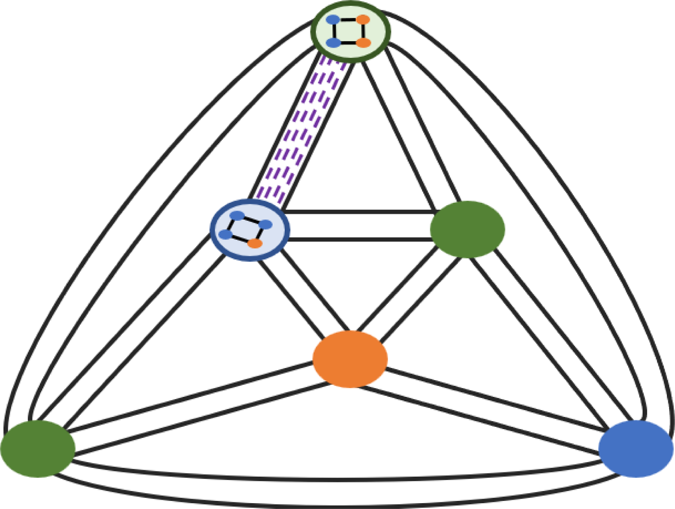
Figure 4. A visualisation of the graph
 $G^2[M_{z}]$
in the case
$G^2[M_{z}]$
in the case
 $t=4,z=2$
and
$t=4,z=2$
and
 $s=2$
. Here, each circle is a copy of
$s=2$
. Here, each circle is a copy of
 $H(t-z,s)$
and the black tubes represent the edges of
$H(t-z,s)$
and the black tubes represent the edges of
 $J(t,z)$
. A pair of copies of
$J(t,z)$
. A pair of copies of
 $H(t-z,s)$
have been displayed, where the vertices of
$H(t-z,s)$
have been displayed, where the vertices of
 $M_{z}$
inside each copy have been coloured according to whether they lie in
$M_{z}$
inside each copy have been coloured according to whether they lie in
 $A'$
(blue) or
$A'$
(blue) or
 $B'$
(orange). Inside the black tube corresponding to the edge of
$B'$
(orange). Inside the black tube corresponding to the edge of
 $J(t,z)$
between this pair of vertices there is some matching, represented by the dashed (purple) edges. Note that this matching may not respect the structure of the
$J(t,z)$
between this pair of vertices there is some matching, represented by the dashed (purple) edges. Note that this matching may not respect the structure of the
 $H$
copies in each circle. Each vertex
$H$
copies in each circle. Each vertex
 $I$
of
$I$
of
 $J(t,z)$
is then coloured according to whether it is
$J(t,z)$
is then coloured according to whether it is
 $A'$
-dominated (blue),
$A'$
-dominated (blue),
 $B'$
-dominated (orange) or evenly balanced (green), corresponding to
$B'$
-dominated (orange) or evenly balanced (green), corresponding to
 $\chi (I)=1,2,$
and
$\chi (I)=1,2,$
and
 $3$
, respectively.
$3$
, respectively.
The edges of
 $G^2[M_{z}]$
then come in two types. Those of type (T1) give rise to a copy of
$G^2[M_{z}]$
then come in two types. Those of type (T1) give rise to a copy of
 $H$
on
$H$
on
 $I \times V(H)$
for each
$I \times V(H)$
for each
 $I \in V(J)$
, whereas those of type (T2) give rise to a matching between
$I \in V(J)$
, whereas those of type (T2) give rise to a matching between
 $I \times V(H)$
and
$I \times V(H)$
and
 $K \times V(H)$
for each
$K \times V(H)$
for each
 $(I,K) \in E(J)$
, where a vertex
$(I,K) \in E(J)$
, where a vertex
 $(I,x)$
is matched to a vertex
$(I,x)$
is matched to a vertex
 $(K,y)$
if and only if
$(K,y)$
if and only if
 $f^{-1}(I,x)$
and
$f^{-1}(I,x)$
and
 $f^{-1}(K,y)$
agree on all coordinates outside
$f^{-1}(K,y)$
agree on all coordinates outside
 $I \cup J$
. Note that this is similar to, but not quite the same as, the Cartesian product of
$I \cup J$
. Note that this is similar to, but not quite the same as, the Cartesian product of
 $J$
and
$J$
and
 $H$
.
$H$
.
We use the partition
 $M_{z}=A'\cup B'$
to define a colouring
$M_{z}=A'\cup B'$
to define a colouring
 $\chi \;:\; V(J) \to [3]$
in the following manner. We say that a copy of
$\chi \;:\; V(J) \to [3]$
in the following manner. We say that a copy of
 $H$
given by
$H$
given by
 $I \times V(H)$
is evenly-split if
$I \times V(H)$
is evenly-split if
 \begin{equation*} \alpha |H| \leq |f^{-1}(I \times V(H)) \cap A'| \leq \left (1-\alpha \right )|H|. \end{equation*}
Note that, since
 $M_{z}=A'\cup B'$
is a partition, if
$M_{z}=A'\cup B'$
is a partition, if
 $I \times V(H)$
is evenly-split then it also satisfies
$I \times V(H)$
is evenly-split then it also satisfies
 \begin{equation*} \alpha |H|\le |f^{-1}\left (I\times V(H)\right )\cap B'|\le \left (1-\alpha \right )|H|. \end{equation*}
If
 $I \times V(H)$
is not evenly-split then we say it is either
$I \times V(H)$
is not evenly-split then we say it is either
 $A'$
-dominated or
$A'$
-dominated or
 $B'$
-dominated if
$B'$
-dominated if
 \begin{equation*} |f^{-1}(I \times V(H)) \cap A'| \geq \left (1-\alpha \right )|H| \qquad \text { or } \qquad |f^{-1}(I \times V(H)) \cap B'| \geq \left (1-\alpha \right )|H|, \end{equation*}
respectively. We then let
 $\chi (I)= 1$
if
$\chi (I)= 1$
if
 $I \times V(H)$
is
$I \times V(H)$
is
 $A'$
-dominated,
$A'$
-dominated,
 $\chi (I)= 2$
if
$\chi (I)= 2$
if
 $I \times V(H)$
is
$I \times V(H)$
is
 $B'$
-dominated, and
$B'$
-dominated, and
 $\chi (I)= 3$
if
$\chi (I)= 3$
if
 $I \times V(H)$
is evenly-split (see Figure 4).
$I \times V(H)$
is evenly-split (see Figure 4).
Let us suppose first that
 $|\chi ^{-1}(3)| \geq \frac{|J|}{\rho t^{2}}$
. In this case, at least
$|\chi ^{-1}(3)| \geq \frac{|J|}{\rho t^{2}}$
. In this case, at least
 $\frac{|J|}{\rho t^{2}}$
of the copies of
$\frac{|J|}{\rho t^{2}}$
of the copies of
 $H$
are evenly-split. As mentioned in Section 2.2, since
$H$
are evenly-split. As mentioned in Section 2.2, since
 $H(t-{z},s)$
is the product of
$H(t-{z},s)$
is the product of
 $t-{z}$
copies of the complete graph
$t-{z}$
copies of the complete graph
 $K_s$
, using (3), we have that
$K_s$
, using (3), we have that
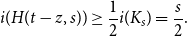 \begin{equation*} i(H(t-{z},s)) \geq \frac {1}{2} i(K_s) = \frac {s}{2}. \end{equation*}
In particular, each copy of
 $H$
which is evenly-split must contain at least
$H$
which is evenly-split must contain at least
 $\frac{\alpha s |H|}{2}$
many edges from
$\frac{\alpha s |H|}{2}$
many edges from
 $A'$
to
$A'$
to
 $B'$
, and so it follows that there are at least
$B'$
, and so it follows that there are at least
 \begin{equation*} \frac {|J|}{\rho t^{2}}\cdot \frac {\alpha s |H|}{2} \geq \frac {\rho |M_{z}|}{t^{2}} \geq \frac {|W|}{t^{2}} \end{equation*}
paths of length 2 between
 $A'$
and
$A'$
and
 $B'$
.
$B'$
.
So, let us assume that
 $|\chi ^{-1}(3)| \lt \frac{|J|}{\rho t^{2}}$
, and so the vast majority of copies of
$|\chi ^{-1}(3)| \lt \frac{|J|}{\rho t^{2}}$
, and so the vast majority of copies of
 $H$
are either
$H$
are either
 $A'$
-dominated or
$A'$
-dominated or
 $B'$
-dominated. Furthermore, since
$B'$
-dominated. Furthermore, since
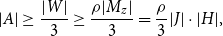 \begin{equation*} |A| \geq \frac {|W|}{3} \geq \frac {\rho |M_{z}|}{3}= \frac {\rho }{3} |J|\cdot |H|, \end{equation*}
it follows that
 $|\chi ^{-1}(1)|,|\chi ^{-1}(2)| \le \left (1-\beta \right )|J|$
. Indeed, if
$|\chi ^{-1}(1)|,|\chi ^{-1}(2)| \le \left (1-\beta \right )|J|$
. Indeed, if
 $|\chi ^{-1}(1)|\gt (1-\beta )|J|$
, then we would have that
$|\chi ^{-1}(1)|\gt (1-\beta )|J|$
, then we would have that
 \begin{align*} |B| &\le |B'| \lt \beta |J|\cdot |H|+ \left (1-\beta \right )\alpha |J|\cdot |H|\\[5pt] &=\frac{\rho }{3}|J|\cdot |H| = \frac{\rho |M_{z}|}{3}\le |A|, \end{align*}
that is,
 $|B|\lt |A|$
, contradicting our assumption that
$|B|\lt |A|$
, contradicting our assumption that
 $|B|\ge |A|$
. Similarly, if
$|B|\ge |A|$
. Similarly, if
 $|\chi ^{-1}(2)|\gt (1-\beta )|J|$
, we would have that
$|\chi ^{-1}(2)|\gt (1-\beta )|J|$
, we would have that
 $|A|\lt |A|$
, a contradiction.
$|A|\lt |A|$
, a contradiction.
Hence, we may restrict our attention to the case where
 $|\chi ^{-1}(1)|, |\chi ^{-1}(2)|\le (1-\beta )|J|$
and
$|\chi ^{-1}(1)|, |\chi ^{-1}(2)|\le (1-\beta )|J|$
and
 $|\chi ^{-1}(3)|\lt \frac{|J|}{\rho t^2}$
. Since, by definition,
$|\chi ^{-1}(3)|\lt \frac{|J|}{\rho t^2}$
. Since, by definition,
 $|\chi ^{-1}(1)|+|\chi ^{-1}(2)|+|\chi ^{-1}(3)|=|J|$
, we have that
$|\chi ^{-1}(1)|+|\chi ^{-1}(2)|+|\chi ^{-1}(3)|=|J|$
, we have that
 \begin{align*} |\chi ^{-1}(1)|,|\chi ^{-1}(2)|\ge |J|-(1-\beta )|J|-\frac{|J|}{\rho t^2}\ge \frac{\beta }{2}|J|. \end{align*}
Hence, by Theorem 14, there is a constant
 $c\gt 0$
such that there are
$c\gt 0$
such that there are
 $c\sqrt{\frac{t}{z(t-z)}}\left (1-\frac{\beta }{2}\right )\frac{\beta |J|}{2}\ge \frac{|J|}{t}$
edges of
$c\sqrt{\frac{t}{z(t-z)}}\left (1-\frac{\beta }{2}\right )\frac{\beta |J|}{2}\ge \frac{|J|}{t}$
edges of
 $J$
which go between a vertex with colour
$J$
which go between a vertex with colour
 $1$
and a vertex with colour
$1$
and a vertex with colour
 $2$
. Each of these edges represents an
$2$
. Each of these edges represents an
 $A'$
-dominated copy of
$A'$
-dominated copy of
 $H$
(which we call the first copy of
$H$
(which we call the first copy of
 $H$
) which is adjacent in
$H$
) which is adjacent in
 $J$
to a
$J$
to a
 $B'$
-dominated copy of
$B'$
-dominated copy of
 $H$
(which we call the second copy of
$H$
(which we call the second copy of
 $H$
). Since at most
$H$
). Since at most
 $\alpha |H|$
of the vertices in the first copy are in
$\alpha |H|$
of the vertices in the first copy are in
 $B'$
and at most
$B'$
and at most
 $\alpha |H|$
of the vertices in the second copy are in
$\alpha |H|$
of the vertices in the second copy are in
 $A'$
, it follows that the number of vertices in the first copy which are in
$A'$
, it follows that the number of vertices in the first copy which are in
 $A'$
and are matched to vertices in
$A'$
and are matched to vertices in
 $B'$
in the second copy is at least
$B'$
in the second copy is at least
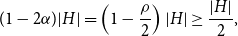 \begin{equation*} (1-2\alpha )|H| = \left (1 - \frac {\rho }{2}\right ) |H| \geq \frac {|H|}{2}, \end{equation*}
since
 $\rho \leq 1$
.
$\rho \leq 1$
.
In particular, there are at least
 \begin{align*} \frac{|J|}{t}\cdot \frac{|H|}{2}=\frac{|M_{z}|}{2t}\ge \frac{|W|}{2t} \end{align*}
many edges in
 $G^2[M_{z}]$
between
$G^2[M_{z}]$
between
 $A'$
and
$A'$
and
 $B'$
and hence
$B'$
and hence
 $\frac{|W|}{2t} \geq \frac{|W|}{t^2}$
many paths of length 2 between
$\frac{|W|}{2t} \geq \frac{|W|}{t^2}$
many paths of length 2 between
 $A'$
and
$A'$
and
 $B'$
in
$B'$
in
 $G$
.
$G$
.
We note that, in terms of showing that the Erdős-Rényi component phenomenon does not hold in irregular product graphs, a simple application of Lemma 16 is sufficient. Indeed, if the
 $G^{(i)}$
are all irregular and of bounded order, then it is not hard to show that there is some
$G^{(i)}$
are all irregular and of bounded order, then it is not hard to show that there is some
 $\epsilon (C) \gt 0$
such that
$\epsilon (C) \gt 0$
such that
 $G$
must contain a vertex of degree at least
$G$
must contain a vertex of degree at least
 $(1+2\epsilon )d$
, and hence by Lemma 16 at a subcritical probability
$(1+2\epsilon )d$
, and hence by Lemma 16 at a subcritical probability
 $p=\frac{1-\epsilon }{d}$
, with positive probability
$p=\frac{1-\epsilon }{d}$
, with positive probability
 $G_p$
will contain a component of order
$G_p$
will contain a component of order
 $d^k$
for any fixed integer
$d^k$
for any fixed integer
 $k\gt 0$
, and so not all components in
$k\gt 0$
, and so not all components in
 $G_p$
have linear order (in
$G_p$
have linear order (in
 $d$
) throughout the subcritical regime. However, Theorem 9 shows that in the particular case of a product of many stars much more is true – in parts of the subcritical regime whp
$d$
) throughout the subcritical regime. However, Theorem 9 shows that in the particular case of a product of many stars much more is true – in parts of the subcritical regime whp
 $G_p$
will even contain a component of order
$G_p$
will even contain a component of order
 $|G|^{1-o_s(1)}$
.
$|G|^{1-o_s(1)}$
.
5. Discussion
In what follows we will use
 $G$
to refer to the product graph,
$G$
to refer to the product graph,
 $t$
for its dimension,
$t$
for its dimension,
 $d$
for its average degree,
$d$
for its average degree,
 $\delta$
for its minimum degree and
$\delta$
for its minimum degree and
 $C$
for the maximum degree of the base graphs. Let us briefly summarise the results on the typical component structure of percolated product graphs with probability close to
$C$
for the maximum degree of the base graphs. Let us briefly summarise the results on the typical component structure of percolated product graphs with probability close to
 $p=\frac{1}{d}$
which follow from Theorems 3 and 6, and Theorems 7, 8 and 9. There are three main assumptions which we work with:
$p=\frac{1}{d}$
which follow from Theorems 3 and 6, and Theorems 7, 8 and 9. There are three main assumptions which we work with:
-
(BO) The base graphs have bounded order;
-
(BD) The base graphs have bounded maximum degree;
-
(R) The base graphs are regular.
Note that clearly (BO) implies (BD).
Lichev [Reference Lichev19] showed that (BD), together with some mild isoperimetric assumptions, is sufficient to show the existence of a linear sized component in the supercritical regime, and to bound the order of the largest component in the subcritical regime. Whilst this bound on the order of the largest component in the subcritical regime was only polynomial in the size of the host graph, we note that Theorem 9 implies that this bound is in fact close to optimal.
Indeed, whilst Theorem 3 implies that when
 $p=\frac{1- \epsilon }{d}$
whp the largest component of
$p=\frac{1- \epsilon }{d}$
whp the largest component of
 $G_p$
has order at most
$G_p$
has order at most
 $\exp \left ( - \frac{\epsilon ^2 t}{9 C^2} \right ) |G|$
, by Theorem 9, there is a choice of
$\exp \left ( - \frac{\epsilon ^2 t}{9 C^2} \right ) |G|$
, by Theorem 9, there is a choice of
 $G$
such that whp
$G$
such that whp
 $G_p$
contains a component of order at least
$G_p$
contains a component of order at least
 $\exp \left (-\Theta ( t) \right ) |G|$
. In particular, (BD) alone is not sufficient to show that the percolated subgraph exhibits the Erdős-Rényi component phenomenon in the subcritical regime (which requires that the largest component in the subcritical regime is of logarithmic order in
$\exp \left (-\Theta ( t) \right ) |G|$
. In particular, (BD) alone is not sufficient to show that the percolated subgraph exhibits the Erdős-Rényi component phenomenon in the subcritical regime (which requires that the largest component in the subcritical regime is of logarithmic order in
 $|G|$
).
$|G|$
).
Furthermore, Theorem 8 further strengthens Lichev’s results in [Reference Lichev19] by greatly weakening the isoperimetric assumptions and showing that at least in the supercritical regime the order of the largest component does behave quantitatively similar to the Erdős-Rényi random graph. As for the order of the second-largest component, Theorem 8 implies it is
 $o(|G|)$
.
$o(|G|)$
.
Question 22.
Is there an example of a product graph
 $G$
which satisfies
(BD)
, and some mild isoperimetric assumptions, for which the second-largest component in the supercritical regime has polynomial order in
$G$
which satisfies
(BD)
, and some mild isoperimetric assumptions, for which the second-largest component in the supercritical regime has polynomial order in
 $|G|$
?
$|G|$
?
As demonstrated by Theorem 6, (BO) and (R) are sufficient to guarantee that the percolated subgraph exhibits the Erdős-Rényi component phenomenon, and Theorem 9 shows that (R) is necessary, in the sense that (BO) without the regularity assumption does not suffice to imply that the Erdős-Rényi component phenomenon holds. However, it remains an interesting open question as to whether (BD) and (R), together with some mild isoperimetric assumptions, are themselves sufficient. For example, the following question is still open.
Question 23.
Let
 $C\gt 1$
be a constant, let
$C\gt 1$
be a constant, let
 $\alpha \gt 0$
be a constant and let
$\alpha \gt 0$
be a constant and let
 $G=\square _{j=1}^{t}G^{(j)}$
be a product graph where
$G=\square _{j=1}^{t}G^{(j)}$
be a product graph where
 $G^{(i)}$
is regular,
$G^{(i)}$
is regular,
 $1 \leq \left |d\left (G^{(i)}\right )\right | \leq C$
for each
$1 \leq \left |d\left (G^{(i)}\right )\right | \leq C$
for each
 $i \in [t]$
and
$i \in [t]$
and
 $i(G) \geq \alpha$
. Does the phase transition that
$i(G) \geq \alpha$
. Does the phase transition that
 $G_p$
undergoes around
$G_p$
undergoes around
 $p= \frac{1}{d}$
exhibit the Erdős-Rényi component phenomenon?
$p= \frac{1}{d}$
exhibit the Erdős-Rényi component phenomenon?
Note that Theorem 7 shows that at the very least (BD) is necessary to show the existence of a linear sized component in the supercritical regime, even under some quite strong isoperimetric constraints. It is perhaps interesting to ask what the limit of this pathological behaviour is. Indeed, the problem here seems to be an abundance of vertices of low degree (where the percolation is locally subcritical), which would suggest that at the very least a probability significantly larger than
 $p = \frac{1}{\delta }$
would be sufficient to show the existence of a linear sized component.
$p = \frac{1}{\delta }$
would be sufficient to show the existence of a linear sized component.
Conjecture 24.
Let
 $G$
be a high-dimensional product graph whose isoperimetric constant is at least inverse polynomial in the dimension, let
$G$
be a high-dimensional product graph whose isoperimetric constant is at least inverse polynomial in the dimension, let
 $\epsilon \gt 0$
, let
$\epsilon \gt 0$
, let
 $\delta \;:\!=\; \delta (G)$
be the minimum degree of
$\delta \;:\!=\; \delta (G)$
be the minimum degree of
 $G$
and let
$G$
and let
 $p = \frac{1+\epsilon }{\delta }$
. Then whp
$p = \frac{1+\epsilon }{\delta }$
. Then whp
 $G_p$
contains a component of size at least
$G_p$
contains a component of size at least
 $(y(\epsilon ) - o(1))|G|$
, where
$(y(\epsilon ) - o(1))|G|$
, where
 $y(\epsilon )$
is defined according to (1).
$y(\epsilon )$
is defined according to (1).
Finally, in the case of
 $G(d+1,p)$
, Theorem 1 can be sharpened to show that, between the subcritical and the supercritical phases, there is a phase when the largest two components are both of polynomial order
$G(d+1,p)$
, Theorem 1 can be sharpened to show that, between the subcritical and the supercritical phases, there is a phase when the largest two components are both of polynomial order
 $|G|^{\gamma }$
for some
$|G|^{\gamma }$
for some
 $\gamma \leq \frac{2}{3}$
, and then a phase when the largest component has order
$\gamma \leq \frac{2}{3}$
, and then a phase when the largest component has order
 $|G|^{\gamma }$
for some
$|G|^{\gamma }$
for some
 $\gamma \gt \frac{2}{3}$
and the second-largest component has order at most
$\gamma \gt \frac{2}{3}$
and the second-largest component has order at most
 $|G|^{\frac{2}{3}}$
, although this whole transition happens in a very small window around
$|G|^{\frac{2}{3}}$
, although this whole transition happens in a very small window around
 $\frac{1}{d}$
(see, for example, [Reference Frieze and Karoński14]).
$\frac{1}{d}$
(see, for example, [Reference Frieze and Karoński14]).

Figure 5. A summary of the typical component structure of percolated high-dimensional product graphs.
It would be interesting to know how the component structure of the graph in Theorem 9 develops as
 $p$
increases, and in particular at what point typically a unique giant component emerges, and when a linear sized component emerges.
$p$
increases, and in particular at what point typically a unique giant component emerges, and when a linear sized component emerges.
Question 25.
Let
 $s$
be a sufficiently large integer and let
$s$
be a sufficiently large integer and let
 $\epsilon \gt 0$
be a sufficiently small constant, let
$\epsilon \gt 0$
be a sufficiently small constant, let
 $G^{(i)}=S(1,s)$
for every
$G^{(i)}=S(1,s)$
for every
 $1\le i \le t$
and let
$1\le i \le t$
and let
 $G=\square _{i=1}^tG^{(i)}$
. Let us write
$G=\square _{i=1}^tG^{(i)}$
. Let us write
 $L_1$
and
$L_1$
and
 $L_2$
for the largest and second-largest component, respectively, of
$L_2$
for the largest and second-largest component, respectively, of
 $G_p$
.
$G_p$
.
-
• For which
$p$
is it true that
whp
$|L_2| = o(|L_1|)$
?
-
• For which
$p$
is it true that
whp
$|L_1| = \Theta (|G|)$
?
-
• Does there exist a probability
$p$
and a constant
$\gamma \gt \frac{2}{3}$
such that
whp
both
$|L_1|$
and
$|L_2|$
have order at least
$|G|^{\gamma }$
?


Furthermore, as mentioned after the proof of Theorem 9, for any family of bounded-order irregular base graphs, the percolated product graph will not exhibit the Erdős-Rényi phenomenon in the subcritical regime, containing a component of order at least a superlinear polynomial (in
 $d$
) for certain subcritical values of
$d$
) for certain subcritical values of
 $p$
. However, in the particular case of Theorem 9, we in fact show that the largest component throughout some part of the sparse subcritical regime, where
$p$
. However, in the particular case of Theorem 9, we in fact show that the largest component throughout some part of the sparse subcritical regime, where
 $p=\Theta (\frac{1}{d})$
, is of polynomial order in
$p=\Theta (\frac{1}{d})$
, is of polynomial order in
 $|G|$
. It would be interesting to know if this behaviour is universal in high-dimensional products of bounded-order irregular graphs.
$|G|$
. It would be interesting to know if this behaviour is universal in high-dimensional products of bounded-order irregular graphs.
Question 26.
For all
 $i\in [t]$
, let
$i\in [t]$
, let
 $G^{(i)}$
be an irregular connected graph of order at most
$G^{(i)}$
be an irregular connected graph of order at most
 $C\gt 0$
. Let
$C\gt 0$
. Let
 $G=\square _{i=1}^tG^{(i)}$
. Let
$G=\square _{i=1}^tG^{(i)}$
. Let
 $\epsilon \gt 0$
be a small enough constant, let
$\epsilon \gt 0$
be a small enough constant, let
 $d\;:\!=\; d(G)$
be the average degree of
$d\;:\!=\; d(G)$
be the average degree of
 $G$
and let
$G$
and let
 $p= \frac{1-\epsilon }{d}$
. Does there exist a
$p= \frac{1-\epsilon }{d}$
. Does there exist a
 $c(\epsilon,C)$
such that whp the largest component in
$c(\epsilon,C)$
such that whp the largest component in
 $G_p$
has order at least
$G_p$
has order at least
 $|G|^c$
?
$|G|^c$
?
The table in Figure 5 summarises what is known about the order of the largest and second-largest component in
 $G_p$
for various values of
$G_p$
for various values of
 $p$
and under various combinations of the assumption (BD), (BO) and (R), and indicates some combinations of probabilities and assumptions where open questions remain.
$p$
and under various combinations of the assumption (BD), (BO) and (R), and indicates some combinations of probabilities and assumptions where open questions remain.


 Open access