


1. Introduction
The design transforms spaces into human experiences, and designers are hence always looking for tools to explore a design space creatively (Buchanan, Reference Buchanan2019). Herein, the ‘design space’ refers to the collection of all possible design options, with the ‘design option’ being the description of all relevant architectural and engineering design aspects. Building performance simulation (BPS) is intended as a tool that enables designers to explore the design space creatively in terms of the building’s performance. BPS allows quantifying the thermal, hygric, acoustic, and so on, behaviour of buildings, most often via a white-box mathematical model deduced from the underlying physics. The exemplary performance prediction model used in this article predicts building designs’ energy performance.
Typically, BPS requires a high amount of information not present in a design, causes too high modelling effort, and is computationally too slow to support designers effectively, that is, not providing instant feedback on options. As a consequence, designers instead rely on rule-of-thumb knowledge (Zapata-Lancaster & Tweed Reference Zapata-Lancaster and Tweed2016). Design decisions based on rule-of-thumb knowledge can be categorized into ‘System 1’ thinking proposed by Kahneman (Reference Kahneman2011). System 1 thinking is usually characterized as autonomous, fast, biased, experience-based, contextual, associative, and so on (Kannengiesser & Gero Reference Kannengiesser and Gero2019). Therefore, decisions based on rule-of-thumb knowledge can result in quick decision-making; however, these decisions often are biased or experienced-based, and may not be valid for the applied design problem (Bleil de Souza Reference Bleil de Souza2012; Zapata-Lancaster & Tweed Reference Zapata-Lancaster and Tweed2016). The computation effort for BPS, along with the different thinking paradigms within the design process, makes it hard to integrate BPS into the design process (Bleil de Souza Reference Bleil de Souza2012; Zapata-Lancaster & Tweed Reference Zapata-Lancaster and Tweed2016).
Machine learning (ML) models developed on simulated data like BPS, also referred to as surrogate models, offer the possibility to develop quick and accurate prediction models (Van Gelder et al. Reference Van Gelder, Das, Janssen and Roels2014). These characteristics of surrogate models facilitate appropriate design support (Østergård, Jensen & Maagaard Reference Østergård, Jensen and Maagaard2016). Recent research results show deep learning (DL) models are outperforming traditional ML algorithms (Singaravel, Suykens & Geyer Reference Singaravel, Suykens and Geyer2018, Reference Singaravel, Suykens and Geyer2019), making DL a potential ML approach for energy performance predictions of building design. Furthermore, methods like transfer learning facilitate DL model reusability (Singaravel et al. Reference Singaravel, Suykens and Geyer2018). Finally, the progressive maturity in DL model development tools allows non-ML domain experts to develop DL models easily, enabling the availability of quick prediction models for design support. Non-ML domain experts, in this context, are domain experts or model developers who typically develop and use performance models of buildings either based on physics or interpretable ML algorithms.
Nevertheless, model explainability is cited as a reason by domain experts to prefer other methods over (DL or other) black-box models for performance predictions (Yu et al. Reference Yu, Haghighat, Fung and Yoshino2010; Reynders, Diriken & Saelens Reference Reynders, Diriken and Saelens2014; Koulamas et al. Reference Koulamas, Kalogeras, Casillas and Ferrarini2018; Batish & Agrawal Reference Batish, Agrawal, Corrado, Fabrizio and Gasparella2019; Foucquier et al. Reference Foucquier, Robert, Suard, Stéphan and Jay2013). Foucquier et al. (Reference Foucquier, Robert, Suard, Stéphan and Jay2013) cite interpretability as one of the reasons to favour physics-based models over black-box methods like artificial neural networks (ANN). Reynders et al. (Reference Reynders, Diriken and Saelens2014) cite the ability of a black-box model to extrapolate is restricted, due to the absence of physical meaning in the learned representation, and proposes a grey-box method for modelling buildings. Yu et al. (Reference Yu, Haghighat, Fung and Yoshino2010) propose a decision tree method for modelling building energy by citing interpretability. Batish & Agrawal (Reference Batish, Agrawal, Corrado, Fabrizio and Gasparella2019) highlight the benefits of ANN for early design stage decision support, but the interpretability of ANN is cited as a limitation. Koulamas et al. (Reference Koulamas, Kalogeras, Casillas and Ferrarini2018) recognizes the interpretability of ANN as a limitation but also highlight the need for experts to develop and interpret results from a physical-based model, and it is difficult for common managers to work with such models.
In this context, explainable artificial intelligence (XAI) gained attention in all its application domains (Barredo Arrieta et al. Reference Arrieta, Díaz-Rodríguez, Del Ser, Bennetot, Tabik, Barbado, García, Gil-López, Molina, Benjamins and Chatila2020). Model explainability is the ability to enable human interpretation of the model itself or model prediction (Ribeiro, Singh & Guestrin Reference Ribeiro, Singh and Guestrin2016; Choo & Liu Reference Choo and Liu2018). Samek & Müller (Reference Samek and Müller2019) categorize model explainability methods into (1) surrogate model-based exploration, (2) local perturbation–based exploration, (3) propagation-based explainability and (4) meta-explanation. Since the utilized DL model is a surrogate model for physics-based BPS, the philosophy behind the surrogate model-based exploration could be applicable. In surrogate model-based exploration, a simple interpretable ML model is used to approximate patterns around a point of interest (e.g., a design option). Interpreting structure within the interpretable ML model provides explainability (Samek & Müller Reference Samek and Müller2019). Similarly, the DL model (also a surrogate model) has learned representations that capture elements of the design- and performance-related structures present within BPS. Exploring the structures within the DL model could highlight patterns that allow us to extract human interpretable information. This exploration is analogous to meta-explanation, which is ‘to better understand the learned representations and to provide interpretations in terms of human-friendly concepts’ (Samek & Müller, Reference Samek and Müller2019).
The human-friendly concept is aimed at non-ML domain experts; hence, it is important to have an exploration method that suits the thinking process of the domain experts. Model explainability is important during model development and design exploration stages. During model development, the explainability of a physical model is obtained by understanding the system model that shows how the information flows within it. Understanding the flow of information within the model and the design problem enables the development of fit-to-purpose models. Similarly, during design space exploration, observing physical parameters and their relation to energy performance within equations in the model gives insights on changes in energy performance as a design parameter is altered. An example of physical parameters in a building energy model is the heat flow rate through walls and other building elements. Model explainability of interpretable ML models is obtained by observing models’ weights or tree structure. In both model classes, experts can reason critically on a model and justify predictions. The reasoning process resembles ‘System 2’ thinking proposed by Kahneman (Reference Kahneman2011) or system thinking presented in Bleil de Souza (Reference Bleil de Souza2012). System 2 thinking is a slower and evidence-based decision-making process (Kannengiesser & Gero Reference Kannengiesser and Gero2019). Systemic thinking is often characterized by (1) utilization of a clear hypothesis to investigate a problem critically and (2) observation of interactions within a model, for example, for BPS, to understand a prediction.
In contrast to physics-based and interpretable ML models (e.g., decision tree, or simple regression), model weights, or the structure within a DL model has no human interpretable meaning. Therefore, this article focuses on a method for non-ML domain experts to obtain model explainability of DL models. As the first step in research, model explainability focusses on the model development stage. However, it is expected that the method can be extended to design exploration as well. The black-box nature causes DL to be close to System 1 thinking process, in which, development relies on experience, rather than justifiable evidence. For instance, DL model development methods like cross-validation (CV), learning curve error-plots give a first impression on how well the model may generalize in unseen data points or design cases. However, the black-box nature of DL fails to facilitate any form of reasoning on generalization, which experts are used to. Understanding generalization is a precondition for the transfer of layers to similar tasks, which are typically done by freezing all hidden layer weights and retraining or fine-tuning the weights of final layers. Furthermore, a wide variety of hidden layer architectures (ranging from fully connected layers to convolutional layers) can be utilized to design a DL model architecture. Even though, non-ML experts can understand how a certain layer architecture works, it can be very difficult to reason why, when, and how many combinations of certain layers are needed. As a result, identifying appropriate DL representations or architectures is subjective and experience-based. Therefore, the proposed method intends to move the development process towards System 2 thinking process by opening DL up for reasoning by means of explainability. The article aims to open up the black box, making it a transparent ‘glass box’. The potential outcome of the explainability method is that non-ML domain experts could explain the following:
(i) The reason why a DL model has good or bad generalization.
(ii) Identify reusable layers during transfer learning applications.
Model explainability for experts are defined as follows:
(i) Explainability for model generalization refers to the ability to observe patterns or trends within the model to infer on model prediction accuracy in unseen design cases.
(ii) Explainability for reusability refers to the ability to identify layers of the model that can be re-used for similar prediction problems.
The next subsections describe the research assumptions, research objectives, and research significance. Section 2 describes the theory of the utilized methods. Section 3 describes the data and models used in this research. Section 4 explains the methodology used to explain the model. Section 5 presents the results and observation of the research. Finally, in Sections 6 and 7, Section 5 findings are discussed and concluded.
1.1. Research assumptions
LeCun, Bengio & Hinton (Reference LeCun, Bengio and Hinton2015) state that ‘deep neural networks exploit the property that many natural signals are compositional hierarchies, in which higher-level features are obtained by composing lower-level ones’. Exploiting the characteristics of compositional hierarchies, DL research in image recognition has shown that convolutional layers capture features relating to the image itself (Chattopadhyay et al. Reference Chattopadhay, Sarkar, Howlader and Balasubramanian2018). In this case, the natural signal refers to the energy demand of a design option, which is the result of interactions at multiple levels. Therefore, it is possible that the hierarchical structure within the DL model captures information about the design space and energy distribution of the design space. In subsequent sections, hierarchical representations pertaining to design space and energy distribution are referred to as design-related interpretations and performance-related interpretation.
Chen, Fuge & Chazan (Reference Chen, Fuge and Chazan2017) showed that a high-dimensional design overlays on a low-dimensional design manifold. Therefore, it is assumed that a high-dimensional building design space can be represented in a low-dimensional space; exploring the low-dimensional representations of the DL model should then highlight interpretations that can be linked to the design space and energy distribution. Methods for dimensionality reduction for model explainability include principal components analysis (Lee et al., Reference Lee, Balu, Stoecklein, Ganapathysubramanian and Sarkar2019; Singaravel, Suykens & Geyer Reference Singaravel, Suykens and Geyer2019), or t-Distribution Stochastic Neighbour Embedding (t-SNE) (van der Maaten & Hinton Reference van der Maaten and Hinton2008). In this paper, low-dimensional representations are obtained through t-SNE.
The low-dimensional representation could only provide intuition on the geometric structure within the model, which, need not be sufficient to explain model generalization. Therefore, mutual information (MI) is used to quantify further the visual observation made on the low-dimensional embedding. Section 2 presents a brief theory of t-SNE and MI.
1.2. Research objectives
The article aims to analyse and present a method that allows non-ML domain experts to interpret and to explain a DL model used in design and engineering contexts. The model interpretability allows non-ML domain experts to infer on model generalization and reusability. Furthermore, model explainability is seen as a means to provide more confidence in the model. The hypothesis tested in this paper is whether the model interpretability of the DL model is obtained by analysing the low-dimensional embedding and MI. In this research, the model interpretation is based on the author’s domain expertise and not based on group experiments. The research questions to address the paper’s objectives are:
(i) What design- and performance-related interpretations are captured during the training process of a DL model?
(ii) How can internal information of a model, especially of hidden layers, help to predict good model generalization?
(iii) How can experts identify reusable layers and justify model generalization?
1.3. Research significance
The article contributes to the application domain of DL. The article shows the exploration of the learned representation within a DL model (a surrogate model for BPS) through t-SNE and MI. The exploration process highlights the organization of the design space within the model. Insights into the organization of the design space allow explaining why a model generalizes in unseen design and identify layers that can be transferred to similar design performance prediction tasks. Such a method for model explainability is an analogy to model explainability methods like layer-wise relevance propagation (Samek & Müller Reference Samek and Müller2019).
The ability to make the above-mentioned explanation on the model will potentially move the model development process (for non-ML domain experts) towards the System 2 thinking paradigm (i.e., evidence-based development). The shift in the way DL models are developed gives a non-ML domain expert the possibility to develop DL models more intuitively, by improving (1) the interpretability of the model as well as (2) the trust in DL methods. Furthermore, the current methods to evaluate model generalization typically confront benchmarking predictions with BPS data, as generating new test design cases through BPS is still possible. However, such benchmarking becomes difficult once the research moves towards a purely data-driven approach, where real measured data (from smart city sensors) that captures all possible scenarios can be limited. In these cases, the model interpretation becomes even more critical, as interpretability allows domain experts to reason on a model.
2. Theory on the methods utilized in the paper
The objective of this section is to give necessary background information on the methods used in this paper so that the results and discussion can be interpreted effectively. This section introduces the DL model analysed for interpretability and the methods to analyses the DL model (t-SNE and MI).
2.1. Architecture of the utilized convolutional neural network (CNN)
A DL model is fed with input features X, which are transformed sequentially by n-hidden layers. The output of the nth hidden layer is utilized to make the final prediction. Figure 1 shows the architecture of the DL model utilized in the paper. The model architecture consists of a sequence of l convolutional layers, followed by a max-pooling layer, k fully connected layers, and an output layer. Each hidden layer transformation results in a vector of hidden layer features  $ {Z}_i\in {\mathbb{R}}^{m_i} $, where mi is the number of hidden features. Section 3.2 presents the information on the number of hidden layers and hidden units in each layer in the model used in this article. The sequential transformations within a DL model comprise of {Z1,…, Zn}, where Z1 and Zn are the hidden features from the first and the last hidden layers, respectively. For simplicity, {Z1,…, Zn} is also referred to as Z act.

Figure 1. Architecture of the CNN for design energy performance prediction.
In this case, input features X is a design matrix, which consists of design features shown in Table 1 paired with physical features inferred based on domain knowledge. The role of the convolutional layer is to filter irrelevant design features for the prediction process. The max-pooling layer retains only the important features for the prediction process. The outputs from the max-pooling layer are mapped to appropriate energy demands Y using fully connected layers. More information on the reasoning for the model architecture can be found in (Singaravel et al. Reference Singaravel, Suykens and Geyer2019).
Table 1. Building design parameters and sampling range.

a Varied differently for each facade orientation.
b U(..): uniform distribution with minimum and maximum; D(..): discrete distribution with all possible values.
2.2. A brief description on t-SNE (t-Distribution Stochastic Neighbour Embedding)
t-SNE generates low-dimensional embeddings of high-dimensional data (van der Maaten & Hinton Reference van der Maaten and Hinton2008). t-SNE is used to understand the features extracted by the DL model (Mohamed, Hinton & Penn Reference Mohamed, Hinton and Penn2012; Mnih et al. Reference Mnih, Kavukcuoglu, Silver, Rusu, Veness, Bellemare, Graves, Riedmiller, Fidjeland, Ostrovski and Petersen2015). Therefore, in this article, t-SNE is used to analyse the learned features of the DL model.
In t-SNE, the low-dimensional embedding is a pairwise similarity matrix of the high-dimensional data (van der Maaten & Hinton Reference van der Maaten and Hinton2008). The high-dimensional data have d dimensions, while the low-dimensional embedding has k dimensions. To allow the visualization of these low-dimensional data, the value of k is either one or two. By minimizing the probabilistic similarities of the high-dimensional data and a randomly initialized low-dimensional embedding, the actual low-dimensional embedding is determined via a gradient-descent-optimization method. In this investigation, instead of such random initialization, the low-dimensional embeddings are initialized to the principal components of the high-dimensional data. The resulting low-dimensional embedding captures the local structure of the high-dimensional data, while also revealing the global structure like the presence of clusters (van der Maaten & Hinton Reference van der Maaten and Hinton2008). Figure 2 illustrates the t-SNE conversion of high-dimensional data with d = 2 into low-dimensional embedding with k = 1. X1 and X2 in Figure 2 (left) could, for example, represent two different building design parameters. Figure 2 (right) shows the corresponding one-dimensional embedding. It can be noted that X embedding obtained through t-SNE preserves the clusters present within the high-dimensional data.

Figure 2. Illustration of t-SNE – Conversion of two-dimensional data (left) into one-dimensional embedding (right).
2.3. Mutual information for evaluating model generalization
Typical applications of MI (also referred with I) are feature selection during model development (Frénay, Doquire & Verleysen Reference Frénay, Doquire and Verleysen2013; Barraza et al. Reference Barraza, Moro, Ferreyra and de la Peña2019; Zhou et al. Reference Zhou, Zhang, Zhang and Liu2019). However, in this article utilizes MI to quantify the ability of a model to generalize in unseen design cases. The reasons for using MI are as follows. Even though the visual interpretation gives insights into a model, engineers typically prefer to work with numeric metrics. Furthermore, current evaluation metrics like mean absolute error percentage (MAPE) provide information on prediction accuracies, and not the complexity of the learned relationship. Knowing the complexity of the learned relationship enables model developers to identify models that balance bias and variance (i.e., underfitting and overfitting).
This section provides the theory to understand model generalization using MI. MI is used in understanding the nature of the learned relationship between input features X and output variables Y. Examples of learned relations are linear or polynomial functions. Figure 3 illustrates the raise in I as the complexity of the learned relationship in a polynomial regression model increases. The model to a degree 5 captures the right amount of complexity between X and Y, as the model with degree 5 has the lowest test mean-squared-error (MSE). In models with degree 1 or 12, X containing too little or too much complexity (or information) about Y, which results in poor model generalization. This section presents a brief intuition on why I increases with high model complexity and the effect of high I on model generalization.

Figure 3. Mean-squared-error (MSE) and mutual information (MI) for different model complexity.
I is a measure of relative entropy that indicates the distance between two probability distributions (Cover & Thomas Reference Cover and Thomas2005), where entropy H is a measure of uncertainty of a random variable (Vergara & Estévez Reference Vergara and Estévez2014). Equation 1 gives the entropy of a random variable X, where, p(X) is the probability distribution of X. A model with high entropy is interpreted as ‘the model that assumes only the knowledge that is represented by the features derived from the training data, and nothing else’ (Chen & Rosenfeld Reference Chen and Rosenfeld1999). Hence, a model with high entropy potentially has the following characteristics: (1) it identifies features that are smooth or uniform and (2) it overfits the training data (Chen & Rosenfeld Reference Chen and Rosenfeld1999).
 $$ H(X)=-\sum_{i=1}^np\left({X}_i\right)\ {\log}_bp\left({X}_i\right) $$
I provides a linear relationship between the entropies of X and Y (Vergara & Estévez Reference Vergara and Estévez2014), estimated through Equation 2. In Equation 2, H(X) and H(Y) represent the entropy of X and Y. H(X,Y) represents the joint entropy of Y and X. I is a non-negative value, in which, I > 0, if there is a relationship between X and Y. When I = 0, X and Y are independent variables. A model with high I can overfit the training data (Schittenkopf, Deco & Brauer Reference Schittenkopf, Deco and Brauer1997). Reasons being (1) the presence of high entropy in the feature space (i.e., X) and (2) the learned relationship is more complex than the required amount of model complexity.
 $$ I\left(X;Y\right)=H(X)+H(Y)-H\left(X,Y\right) $$
Therefore, the following deductions are expected in a DL model for different complexity of the learned features Z act. Ig refers to the I in model with good generalization and Ip refers to the I in model with poor generalization.
1. Z act is too complex (i.e., overfitting), Ig < Ip;
2. Z act is too simple (i.e., underfitting), Ig > Ip.
3. Developing DL model for explainability analysis
During the model development stage, multiple models with several hyper-parameter configurations are tested before selecting a model for actual design performance prediction. The model with the lowest test error is assumed to generalize well, the one with the largest error to poorly generalize. By comparing the learned features of the DL model with good and poor generalization, the underlying structure for generalization could be observed. This section presents (1) a brief description of the training and test data and (2) the test accuracies of the models used in the explainability analysis.
3.1. Training and test design cases
In this article, data are obtained from BPS instead of real data from smart building or lab measurements. The reason for this choice is today’s limited availability of pairs of design feature X and performance data Y like energy. Currently, data collected from smart homes are mainly focused on performance variables. Without information on corresponding X, it is difficult to develop a representative model for design. However, in the future, it could be possible to have design performance models based on real data.
The exemplary BPS applied in this paper specifically captures the energy behaviour of an office building located in Brussels (Belgium). Energy performance data for training and test design cases are obtained through parametric BPS performed in the EnergyPlus software (EnergyPlus 2016). In this article, energy performance is determined by the cooling and heating energy demand of the office building. Peak and annual energy demand further characterize these cooling and heating energy demands. Figure 4 shows the training and test office design cases with a different number of stories. The design parameters sampled in the simulation models are shown in Table 1. Such typical design parameters are discussed during the early design stages. Hence, the utilized model is representative of the early design stages. The applicability of the model for other design stages have not been researched and is out of scope for the current article. The samples are generated with a Sobol sequence generator (Morokoff & Caflisch Reference Morokoff and Caflisch1994). The training data consists of 4500 samples, whereas each test design case consists of 1500 samples.

Figure 4. Training and test design cases.
Figure 4 shows the form of the building design used in the training and test design cases. The training cases are from buildings with 3, 5, and 7 storeys. The test design cases are from 2, 4, 8 to 10 storeys. Variation in the number of storeys varies the environmental effects like solar gain on design performance. It can be noted from this figure that, only the four-storey building is within the interpolation region of the building form and environmental effects on the design. Other building design options are in the extrapolation region in relation to building form and environmental effects. Therefore, the test cases observe the generalization beyond the training design cases (in terms of building form).
3.2. Utilized DL models for the explainability analysis
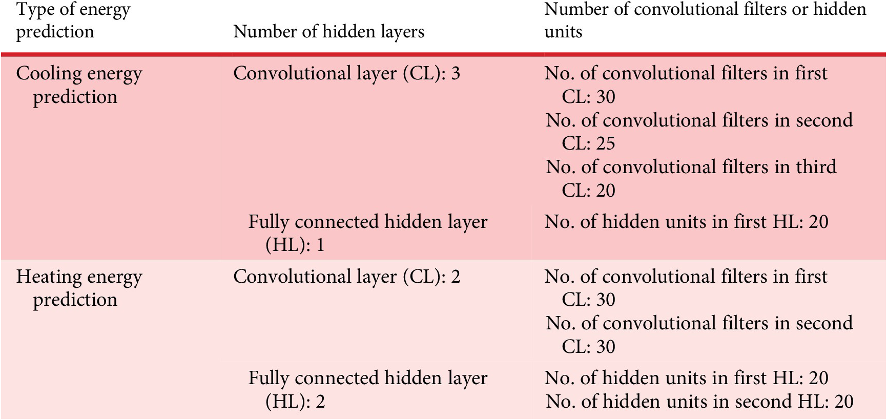
Table 2 shows the utilized CNN architectures for cooling and heating energy predictions. The hyper-parameters are derived after manual tuning through CV accuracy. In this case, CV data are a subset of training design cases that were not part of the training process. The parameters tuned were the number of convolutional and fully connected hidden layers and the hidden units in each layer. The choice for the parameters is based on a manual search process. The first step of the search process was the identification of the required number of convolutional and fully connected hidden layers for predicting cooling and heating energy. The identification of the required number of hidden layers gives an idea of the required model depth to capture the problem. Subsequently, the hidden units are tuned manually till low CV error is observed.
Table 2. Architecture of the deep learning model.
Identify models and explaining generalization are done by comparing different models. Therefore, explainability for model generalization requires models that generalize well and poorly. The training space of a DL model contains multiple optima. Therefore, for the parameters defined in Table 2, the training loop is repeated for 100 iterations. In each iteration, model weights are initialized randomly, and the 100 trained models are saved for analysis. The resulting 100 models should have different generalization characteristics. In this study, MAPE is used to select the models because, for the current data, this metric provided more insights into the model performance than other metrics like the coefficient of determination. For the trained models, a model with the lowest and highest test MAPE is considered models with good and poor generalization.
Figures 5 and 6 show the cooling and heating models test MAPE for 100 independent training runs. Figure 5 (top) shows the test MAPE for peak cooling energy predictions, Figure 5 (bottom), for total cooling energy predictions. Similarly, Figure 6 (top) shows the test MAPE for peak heating energy predictions, Figure 6 (bottom), for total heating energy predictions. These figures show that most of the models converge in optima that generalize well (i.e., test MAPE lower than 20%). However, good model generalization for the cooling model (green bar-chart in Figure 5) and heating model (green bar-chart in Figure 6) is observed only after 30 independent training runs, indicating the influence of random initialization in each training run. The chances of model convergence in a suboptimum that generalizes poorly are also high, indicating that models need to be selected after robust testing. Section 5 analysis these models based on the methodology presented in Section 4.

Figure 5. Cooling model test mean absolute percentage error (MAPE) in 100 training runs. The models highlighted in green, generalized well and poorly. The highlighted models are used in Section 5.2 for analysis.

Figure 6. Heating model test mean absolute percentage error (MAPE) in 100 training runs. The models highlighted in green, generalized well and poorly. The highlighted models are used in Section 5.2 for analysis.
4. Methodology to explain DL model during model development
The objective of this methodology is to enable model developers to explore the model to understand the structure present within the model. Understanding the underlying structure gives insights on model behaviour, which allows for interpretability on model generalization and reusability. The analysis is performed in three stages, which are (1) understanding the geometric structure learned by the model through t-SNE, (2) comparing the learned geometric structure of a model with good and poor generalization and (3) understanding the nature of the learned information through MI. The three stages performed sequentially increases model interpretability for generalization and reusability. Each of the following stages is intended to add structure to Z act, which in total results in model interpretability for model developers.
4.1. Understand the basic design and performance by the model
The objective of this stage is to understand which transformations in Z act can be linked to design features and performance parameters. Linking transformations within Z act to human interpretable design and performance interpretations gives the model developers a visual understanding of the learned structure. Furthermore, visualizing a model enables system thinkers to pose hypothetical questions to verify if the visual interpretation is correct. An example of a hypothetical question is, how does the model characterize a design option with low energy demand?
For this analysis, a model that is categorized as a good generalization is utilized. For all the training design cases, t-SNE converts high dimensional X and Z act to one-dimensional embedding. The input feature embedding x embedding $ \in {\mathbb{R}}^{k=1} $, and hidden layer embedding z act-embedding = {z1, …, zn}, where z act-embedding
 $ \in {\mathbb{R}}^{n\times k=1}. $ Two-dimensional dependency plots between x embedding, z act-embedding, and the output variable show the information flow within the model. The dependency plots are overlaid with information of design parameters, and markings of design options with high and low energy demands. Analysing the information flow within the model along with design and energy-related information gives the model developer a basic intuition on the learned structure. The understanding learned structure is expected to provide insights on model reusability.
4.2. Compare the learned geometric structure for a model with good and poor generalization
In this stage, the initial model understanding is extended to visually understanding the models that generalized good and poorly. In this stage, models that have low test MAPE and high test MAPE are utilized. For the selection models, the steps from Stage 1 are repeated. By comparing the dependency plots for the model with good and poor generalization, model developers can get insights into how the internal structure influences the model behaviour, in terms of model generalization.
4.3. Understand the nature of the learned information through MI
Stages 1 and 2 focused on the visual understanding of the model structure. In this stage, MI information is analysed between Zn (i.e., hidden features from last hidden layer) and Y within the training design cases. Understanding MI within training design cases reduces the limitation on selecting a model based on the chosen test data. Incorporating Zn in estimating MI includes model complexity in the evaluation process of model generalization. Analysing MI based on the relationship between Ig and Ip (defined in Section 2.3) allows determining the nature of the learned complexity. Insights from MI, along with insights from Stages 1 and 2, give model developers the ability to explain the model. The methodology to estimate MI for all the developed models (i.e., 100 models developed in Section 3.2) are:
(i) Zn comprises of {Zn1,…., Znm}, where m is the number of features in Zn. m also corresponds to the number of hidden units present in the final hidden layer (see Table 2). MI between all features in Zn and Y is estimated.
(ii) Total MI of the hidden feature space is estimated as it allows a direct comparison of multiple models. Total MI of the feature space is estimated by
 $ {\sum}_{M=1}^mI\left({Z}_{nm};Y\right) $.
(iii) Comparing Ig and Ip, along with test MAPE and visual analysis, gives insights into how a model generalizes in unseen design cases.

5. Results and observations for model explainability for model developers
5.1. Visual explanation of the learned design and performance geometric structure
Figures 7 and 8 show the low-dimensional embeddings for, respectively, the cooling and the heating model. In Figures 7a and 8a, building design parameters are represented by x embedding. Figures 7a–f and 8a–f show the sequential transformation of x embedding within the DL model. For the cooling model, z act-embedding consists of the embedding of three convolutional layers CL1-3 embedding, of one maxpooling layer Maxpoolingembedding, and of one hidden layer HL1 embedding. Similarly, for the heating model, zact-embedding consists of the embedding of two convolutional layers, of one maxpooling layer and of two hidden layers.

Figure 7. Cooling model: Low-dimensional embedding overlaid with information about building design with different types of chiller. The black star and dot correspond to designs with low energy demand. Similarly, the red star and dot correspond to design options with high energy demand. Table 3 shows the engineering description of the highlighted design options.

Figure 8. Heating model: Low-dimensional embedding overlaid with information about building design with different types of the boiler pump. The black star and dot correspond to designs with low energy demand. Similarly, the red star and dot correspond to design options with high energy demand.
Figure 7 is overlaid with information of chiller types in the design space. The cyan-colored cluster shows building design options with an electric screw chiller, and the blue-colored cluster shows the options with an electric reciprocating chiller. Figure 8 is overlaid with information about boiler pump types in the design space: the green and yellow cluster respectively show the building design options with constant and variable flow boiler pump.
In Figures 7a and 8a, the relationship between x embedding and CL1 embedding is shown. Figures 7a and 8a highlight the presence of two dominant clusters within the design space. The first convolutional layer in cooling and heating models learned to separate the design space based on chiller type and boiler pump type. As this information flows (i.e., CL1 embedding) within the model, design options are reorganized to match the energy signature of the design.
The reorganization of design based on energy signature is observed when Figures 7 and 8 are viewed from figures f to figures a. In Figures 7f and 8f, low values of embedding from the final-hidden layer correspond to low-energy demands of the building design space and vice-versa. As we move from figure f to figure a, the design space is reorganized based on chiller type or boiler pump type.
It can also be noted from Figures 7a,b and 8a,b that the nature of the clusters for the cooling and heating models are similar. This could be due to the nature of the different cooling and heating energy behaviour for the same design option. For example, the chillers utilized in the design options (i.e., screw or reciprocating) have different behaviour on energy, when compared to the same boiler with different types of pump. Such factors, combined with other design parameters, results in differently clustered representations within the convolutional layers.
To further verify if the model is indeed reorganizing the design space, four design options are selected (see Table 3 for the cooling model). In Figures 7 and 8, these design options are shown with star and dot represent the type of chiller or boiler pump. Design options marking with red color represents high-energy-consuming design options while marking with black color describes low-energy design options. It can be observed from Figures 7 and 8, as design information flows within the DL model, the design options are moved towards their respective energy signature.
Table 3. Design options highlighted in Figure 7.

A closer observation of the design parameters of the selected design options further confirms the reasons for the low and high energy demands. Designs 1 and 3 in Table 3 are small buildings compared to Designs 2 and 4. Hence, Designs 1 and 3 have a smaller energy signature. Looking at the building material propertiesFootnote 1 of Designs 1 in Table 3 shows a building design option will have high heat gains. However, the building has low cooling energy demand, as the chiller coefficient of performance (COP) is high. However, Design 3 has a chiller COP lower than design one but has similar energy signatures. The reason being, Design 3 has no windows (WWR = 0.01), which removes the effect of solar gains. Hence, the absence of a window allows us to justify why the design option has a low-energy signature. Of-course, Design 3 is not a realistic design option. Design 3 is used in the training data to increase the captured dynamic effects. Similar, observations can be made for the heating model’s design options. Model developers with a background of BPS can logically reason with such observations, hence increasing model explainability for model developers with a non-ML experience.
The global structure within the model is that the DL model’s features learned to reorganize the design options with respect to their energy signature. The process of reorganization takes place in n steps, where n is the number of hidden layers in the model. In this case, the learned features can be viewed as the DL model’s n-stepwise reasoning process to determine the energy demand of a building design option. For instance, the first convolutional layer features learned (see Figure 7a) ‘how to segregate design options based on the utilized types of chiller’. The second and third convolutional layers learn (see Figure 7b,c) ‘within a chiller type, how can design options be reorganized based on their energy signature’. This reasoning is indicated by the tighter organization of design options in Figure 7c when compared to Figure 7b. Similarly, Figure 7d–f shows that the layers features learn to reason ‘how to reorganize the design options representative of the energy signature of the design’. Similar to the cooling model, in Figure 8a, the first convolutional layer CL1embedding in the heating model learned features that segregate the design options based on the boiler pump type. The subsequent layer (see Figure 8b–f) learned to reorganize the design space that reflects the heating energy signature of the design option. In Section 5.4, how the stepwise reasoning process adds explainability is discussed. In the next section, the low-dimensional embeddings from a model with good and poor generalization are compared.
Within the global structure, two distinct geometric structures are observed. The structures are design- and performance-related interpretations. The convolutional layers learn to segregate based on the design space (e.g., see Figure 7a). Analysing other design parameters within the convolutional layers embeddings indicated a similar logical organization of the design space. Therefore, model representations until the max pooling layer can be considered as representations related to design-related interpretations. Similarly, the fully connected layers hidden layers learn to organize based on the design feature map (i.e., the output of a max pooling layer) based on the energy signature of the design space. Therefore, fully connected hidden layers can be considered performance-related interpretations. Section 5.4 discusses how model developers can use this information.
5.2. Comparing the learned geometric structure for models with good and poor generalization
Figure 9 (top) and Figure 10 (top) illustrate the low-dimensional embeddings for models with good generalization, while Figure 9 (bottom) and Figure 10 (bottom) show these embeddings for models with poor generalization. Observing the top and bottom graphs in Figures 9 and 10 shows that, irrespective of the model’s ability to generalize, the models learn to perform a sort of stepwise reasoning process. Furthermore, Figure 9d (top) and Figure 9b (bottom) are similar patterns learned by different layers in the model architecture. A similar observation can be made in Figure 10e (top) and Figure 10d (bottom). Indicating that purely understanding learned geometric structure does not give insights into model generalization.

Figure 9. Cooling model: Low embedding’s dependency plot overlaid with information of chiller type (top) model with good generalization (bottom) model with poor generalization.

Figure 10. Heating model: Low embedding’s dependency plot overlaid with information of the boiler pump type (top) model with good generalization (bottom) model with poor generalization.
The figures also indicate that for the model with good generalization, the low-dimensional embedding has a higher variability. In contrast, the model with poor generalization has a low-dimensional embedding that is tighter, less variable. The observation for low variability or smoothness can be an indication of high entropy (based on the theory presented in Section 2.3), which is also an indication of overfitting. The estimation of MI in the next section confirms this observation.
5.3. Understanding mutual information between learned features and energy demand
Figure 11 shows the MAPE for all test design cases against the MI for all training design cases obtained from different DL models in the 100 training runs. Figure 11 (top) shows the results obtained from the cooling model in which the red points show the models analysed in the above section. Similarly, Figure 11 (bottom) shows the results from the heating model, and the blue points represent the models analysed in the above section. It can be noted from these figures that the model that generalized the most does not have the highest nor the lowest MI. Therefore, a model with good generalization captured the right amount of information and learned the required complexity. However, based on MI, it is difficult to identify the degree of learned complexity.

Figure 11. Test mean absolute error percentage (MAPE) versus mutual information (top) for the cooling model, (bottom) for the heating model. The cross in the figures highlights the MAPE and mutual information (MI) for a model with good generalization. It can be noted from the cross that a model with good generalization has neither low nor high MI.
In Figure 11 (top), the cooling model with good generalization has an I g of 8.9 and 8.4 for peak and total cooling energy. While for the cooling model with poor generalization, the I p is 90.6 and 100.95 for peak and total cooling energy. In Figure 11 (bottom), the I g for the heating model with good generalization is 11.6 and 10.41 for peak and total heating energy. While the I p for the heating model with poor generalization is 40.32 and 19.29. For both heating and cooling models, I g is lower than I p. Higher Ip confirms, the visual observation in the above section, that the model with poor performance has maximized entropy between X and Y. Finally, higher Ip indicates that the learned relationship is more complex than needed.
5.4. Model explainability for model developers
Explainability for re-usability is achieved when model developers can identify re-usable aspects of a specific model. A method for model re-usability is transfer learning. In transfer learning, typically, the final layer is re-trained or fine-tuned to meet the needs of the new prediction problem. The above insights can be utilized as follow:
(i) Transferring the DL model to similar performance prediction problem:
a. In this case, layers categorized under design-related interpretations are frozen and layers categorized under performance-related interpretations are retrained or fine-tuned. Therefore, the convolutional layers can be frozen, and fully connected layers can be retrained or fine-tuned.
(ii) Transferring the DL model to other design cases with similar energy distribution:
a. In this case, layers categorized under performance-related interpretations are frozen and layers categorized under design-related interpretations are retrained or fine-tuned. Therefore, the convolutional layers can be retrained, while keeping the fully connected layers frozen.
Other re-usability cases can be developing components that capture design and performance related interpretations. Such components can increase the use of DL models in design. Further research on model re-usability based on explainability analysis needs to be done.
Explainability for generalization is the ability of the developer to infer on prediction accuracies in unseen design cases. During the model development stage, comparing the low dimensional embedding and MI for different model gives more insights on model generalization in unseen design cases. However, analysing the model with embedding space and MI is additional to the current development methods like CV and learning curve. Explainability for generalization is obtained as follow:
(i) The tight organization of the low-dimensional embeddings (see Figure 9d–f (bottom) and Figure 10d–f (bottom) indicated that the models with poor generalization have low dimensional embeddings that are smoother in nature. The smoothness brings the different design options very close to each other and characterizes high entropy which is confirmed by high MI value. This observation indicates that the learned relationship is too complex for the given problem or the model is overfitting.
(ii) The stepwise reasoning process shows how design moves within a model, and convolutional layers are categorized under design-related interpretations. Therefore, for a given design option, the developer can compute the pairwise distance between the design feature map (i.e., the output of the max pooling layer) for the evaluated design and training design cases. The pairwise distance indicates the closeness of design to the training design cases. Therefore, the model developer can be confident in the predictions when the pairwise distance is low, and skeptical when the pairwise distance is high.
Through the above method, model developers can identify design- and performance-related interpretations within the model. The identified interpretations allow model developers to identify re-usable elements and infer on model generalization.
6. Discussion
The research started with the hypothesis that model interpretability for model developers can be obtained by analysing it through the low-dimensional embedding and MI. Results are shown in Figures 7 and 8, during the training process, the model learns an n-stepwise reasoning process. The learned n-stepwise reasoning process is the reorganization of the design options based on their energy signature. Furthermore, analysing the model by overlaying design parameters and tracking a few design options, indicates that the model can be divided into two regions, which are design and performance parameter related. The segregation of models into two regions will allow model developers, in different cases, to identify re-usable layers within the model. Furthermore, comparing the low-dimensional embedding and MI of multiple models will allow identifying the model’s ability to generalize in unseen design cases. Such an exploration of the model can enable developers to pose different questions to understand the structure within the model. Understanding the structure can result in the ability to infer model behaviour in a different context. Finally, the ability to infer the model structure (i.e., n-stepwise reasoning process and design- and performance-related interpretations) potentially adds model interpretability to non-ML model developers. The current model interpretation is based on the authors’ domain knowledge, further group experiments are needed to verify if more domain experts agree with this interpretation.
Engineers are used to developing system models like BPS based on multiple sub-models called components in modelling languages like Modellica (Hilding Elmqvist 1997). Typically, the components are typically physics-based or interpretable ML models. However, the utilized components could be a DL model as well. Since, the DL model captures two distinct behaviours, which are design- and performance-related interpretations. It would be possible to have components of design- and performance-related components. Design-related components position the design option in relation to the design space, and performance-related components map the position of the design option in the design space to a performance prediction. Therefore, the performance-related component’s interfaces with physics-based components and design-related components could interface between other performance-related components. For instance, a design-related component developed on cooling data could potentially interface with the heating model’s performance-related layers. Another example could be a design-related component could represent design’s with varying complexity or level of detail, while interfacing with a performance-related component developed. In this way, model developers could reuse existing models. The efficacy of this re-usability needs to be researched further. However, model interpretability remains the central link to move towards the steps of re-usable black-box components.
In this article, model interpretability relied on a visual understanding of low dimensional embeddings and MI. The visual observation is further verified by observing the flow of the design options within the low dimensional embeddings. Later, MI is used to understand the reason for the smoothness in the low dimensional embeddings. Such verification by questions or through metrics like ML on the visualization is critical to avoid a biased interpretation. Furthermore, effective interpretation is only possible by or in collaboration with a domain expert, they will be able to ask critical questions and easily spot common or logical patterns in the analysis.
The method used for analysing the model appears to have the characteristics of System 2 thinking, which is evidence-based reasoning. Evidence is obtained by (1) posing question on how a design will be transformed within a model, (2) comparing embeddings of good and poorly generalized models and (3) using MI to validate the observations. In contract, traditional development methods through CV and general rules for reusability appear to have characteristics of System 1 thinking, as development is mainly based on experience. A consequence of System 2 thinking is the model development process can become slower, as developers need to perform mental simulations on the analysis results in a relationship with the domain knowledge. Furthermore, analysing the models through the proposed method is model agnostic, that is, the method applies to any model architecture. Therefore, non-ML developers could use AutoML techniques to tune-hyper parameters and develop multiple models in an automated fashion. For the developed models, the model developer can analyse the learned model structures. Therefore, effective person-hours for model development could remain similar. It must be noted that the current AutoML methods might not be sophisticated enough to work autonomously. It is expected that in the future, such an approach could become feasible.
The visual analysis is performed for a DL model has five hidden layers. The visual analysis could become mentally difficult when the number of hidden layers becomes larger. In such cases, the visual analysis could be done for groups of layers, to identify the learned structure. The effectiveness of such grouping needs to be evaluated further. Furthermore, in this article, each high dimensional layer is reduced to a one-dimensional embedding, which could have removed other interesting insights. Therefore, methods to extract finer details in a high dimensional space needs to be developed. A potential approach is to apply clustering methods on hidden layers, which are followed by sensitivity analysis on hidden features with respect to design parameters and performance variables. Information on the behaviour of the clusters (obtained through sensitivity analysis) could give insights into the structure of the model, but all highlight interesting insights into the domain. Insights into the domain could be interesting when the domain under investigation is still actively being researched, and our knowledge is not complete.
Through the proposed approach, model developers can potentially understand the model. However, it is important to explore; further, the willingness and the level of intuition the above method gives to developers who like and use white- and grey-box approaches. This is important because the language used to understand a DL model is based on patterns and distances in abstract space (like hidden features) that are interpreted through its relation to design parameters. In contrast, the language used to understand white- or grey-box models is based on patterns in the physical space (like heat flows, humidity levels) in relation to design parameters. The fundamental difference in the language to communicate and understand a model could be even more limiting, once black-box models can be interpreted in greater precision. Therefore, it could be interesting to analyses methods that could add a physical meaning to the abstract space.
However, at a design team level, interpretation of the abstract space could be more interesting. The reason being, the members of a design team, have not only different thinking paradigms but also utilize different language to communicate concepts and ideas. If the team members have a multi-disciplinary thinking process, the communication will be smooth. Else, communication and design collaboration become harder. This raises an interesting question, would the interpretation of an abstract space promote a common design language or facilitate design communication and collaboration? Further research on adding physical interpretation to abstract space or using abstract space to promote design communication should be researched and developed.
Even though, this article focused on interpretability for generalization and re-usability, another important aspect for non-ML domain experts is to explore the design space and justify the recommended design strategy. Justifications could be obtained by visualizing the evaluated design embeddings together with training design case embeddings to get insights on the energy characteristics of the design’s options neighborhood. These insights along with domain knowledge could allow an expert to formulate appropriate justifications. Furthermore, the DL model is easily differentiated through automatic differentiation (AD) methods. During the training process, AD methods are used to compute gradients to update model parameters. The same approach is used to compute gradients with respect to design features X. Information on the gradients could allow the domain expert to explore the design space, and also identify design changes to improve a poorly performing design option. The effectiveness of the design steering process through gradients, and justification by observing neighborhoods of design embeddings needs to be researched further.
7. Conclusions
It has been observed that the DL model has learned to sort/rearrange the design space corresponding to its energy signature. Each transformation within the model moves the design towards the appropriate location of the data distribution giving an interpretation of the DL model. Incorporating such methods within the model development process could increase the confidence of model developers with domain expertise other than ML. Furthermore, domain experts can look at the model more critically. Enabling the development of novel training methods.
Features extracted by the DL model do not have any physical meaning. However, the study shows the presence of a logical principle behind the transformations. The DL model utilized in this article showed it has learned an n-stepwise reasoning process, which is to sort the design space (in n-steps) in accordance with the energy distribution of the design space. Engineers (in this case, the domain experts) may find this explanation abstract. However, architects in the design team could find such reasoning more concreate as the explanation is in relation to the design space and not physical parameters like heat transfer. For example, reducing the window area moves the design towards design options with overhangs and larger windows. Therefore, it is hypothesized that explainable DL models with high prediction accuracy will facilitate the integration of the different thinking paradigms of engineers and designers/architects. Furthermore, the need for experts to interpret model results, within the design process, could be reduced due to the abstract nature of the DL model interpretations and allow architects to use the models directly. Reducing the need for experts will benefit small building design projects with low budgets while enabling the design team to follow a model-based design process.
The human interpretable meaning to the extracted features could encompass the needs of different thinking paradigms. For example, for a certain hidden activation, engineers are presented with insights on physical parameters, and architects are presented with neighboring design options within the design space. Allowing for a meaningful insight into design performance through DL. This, in turn, can result in effective collaboration between a designer and an engineer during the design process. Furthermore, such generic insights obtained from the transformations of a DL model could play a vital role in the creative process of a designer. More research needs to be done in identifying methods for integrating designers and engineers through DL.
Glossary
- AD
Automatic Differentiation
- BPS
Building Performance Simulation
- CL
Convolutional Layer
- CNN
Convolutional Neural Network
- CV
Cross-Validation
- DL
Deep Learning
- H(X)
Entropy of X
- Q’ equip
Equipment Heat Gain
- c floor
Floor Heat Capacity
- HL
Fully Connected Hidden Layer
- U floor
Ground Thermal Conductivity
- h
Height
- {Z1,…, Zn} or Z act
Hidden Features
- n air
Infiltration Air Change Rate
- X
Input or Design Features
- l
Length
- Q’ light
Lighting Heat Gain
- ML
Machine Learning
- MAPE
Mean Absolute Error Percentage
- MI or I
Mutual Information
- Ig
Mutual Information for a Model with Good Generalization
- Ip
Mutual Information for a Model with Poor Generalization
- n floor
Number of Stories
- α
Orientation
- Y
Output Variable or Performance Variable
- l oh
Overhang Length
- p(X)
Probability of X
- U roof
Roof Thermal Conductivity
- t-SNE
t-Distribution Stochastic Neighbour Embedding
- U wall
Wall Thermal Conductivity
- w
Width
- g win
Window Solar Heat Gain Factor
- U win
Window Thermal Conductivity
- WWR
Window to Wall Ratio
Acknowledgements
The research is funded by STG-14-00346 at KUL and by Deutsche Forschungsgemeinschaft (DFG) in the Researcher Unit 2363 “Evaluation of building design variants in early phases using adaptive levels of development” in Subproject 4 “System-based Simulation of Energy Flows.” The authors acknowledge the support by ERC Advanced Grant E-DUALITY (787960), KU Leuven C1, FWO G.088114N.


 Open access