


1. Frame of reference
While one aspect of this article is on modelling coupling in design decisions required for designing connected systems, another aspect is to improve the validity and usefulness of decisions undertaken by identifying and addressing the effect of uncertainties. Designing a connected engineered system requires a designer to ascertain critical decisions and model their interactions. It is crucial to ascertain critical decisions and model their interactions, allowing for the coupled representation of connected engineered systems using the multiple interacting decisions. Such a coupled representation simplifies the realisation of connected engineered systems, which is crucial for designing such systems. Our view of a connected engineered system consists of numerous interacting design decisions that cannot be taken by disregarding the influence of one decision on other decisions. For instance, a gearbox is a mechanical transmission unit containing integrated gears that provide torque and speed conversion among rotating equipment. The design process associated with a gearbox requires solving several problems through several stages. In essence, these stages involve decision-making as a result of analysis involving design calculations (static, fatigue, thermal and vibration), materials, manufacturing, economics, and so forth. The results of the analyses govern the decisions, and the decisions in themselves are interrelated; that is, one decision is likely to influence other decisions. To effect better decision-making in the design of such engineered systems, it is imperative to:
-
(i) Identify critical decisions for designing such systems.
-
(ii) Identify analyses from various knowledge domains that govern the decisions.
-
(iii) Identify and model how these decisions interact.
However, to undertake such coupled decisions, we rely on the models that are an abstraction of reality and are typically incomplete and inaccurate and incorporate different levels of fidelity. This requires identifying robust solutions away from the boundary solutions (optimal) that are relatively insensitive to the effect induced when the inherent assumptions in models do not hold. This is even more critical when numerous interacting decisions ensure that the cumulative effects of incompleteness and inaccuracies in each decision do not guide us to an infeasible decision. On the other hand, design decisions that rely on computer simulations do not account for uncertainties induced by noise factors (uncontrollable parameters), design variables (controllable parameters), the model approximations used in creating simulation models or uncertainty propagation across different length and time scales (Choi et al. Reference Choi, Austin, Allen, McDowell, Mistree and Benson2005; Allen et al. Reference Allen, Seepersad, Choi and Mistree2006). Similarly, uncertainties in experimental data arise as a result of strong dependencies on the environment, methodology and equipment involved in the experiment. Therefore, uncertainty management methods are critical to enable the development of robust design methods. This necessitates studying the source of these uncertainties and developing appropriate methods to address them. To manage uncertainties and effect robust decision-making, robust design principles are to be integrated. To enable robust decision-making in a coupled decision environment, the gaps identified, and relevant hypothesis are as follows:
Gap 1 A method to design using coupled design decisions is needed.
Hypothesis 1 By establishing criteria to classify design decisions, we develop a method to study and model coupling in design decisions. As an outcome, a decision classification scheme, Multilevel Decision Scenario Matrix (MDSM), is created. Depending on the number and nature of decisions, decision interaction and levels in decisions, different decision scenarios are created using MDSM to formulate a specific design problem. In this article, one instance of a decision scenario is demonstrated for the robust design of a one-stage gearbox.
Gap 2 A method to explore robust solutions to coupled design decisions that are relatively insensitive to uncertainties by relying on typically incomplete and inaccurate models and incorporate different levels of fidelity is needed. Managing the effect of uncertainties is therefore critical to ensure the validity and usefulness of the design decisions and, hence, improve the design’s quality and reliability.
Hypothesis 2 By incorporating robustness metrics [design capability index (DCI) and/or error margin index (EMI)] as design goals and constraints in the coupled decisions, we enhance the usefulness and validity of design decisions by managing uncertainties.
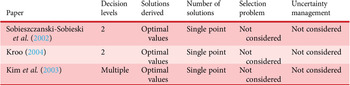
Before we present our approach, we discuss three papers that are foundational to the work we are presenting: the design of coupled systems (see Table 1). Bi-level integrated system synthesis (BLISS) applies a decomposition-based approach whereby optimisation of a complicated engineered system is carried out by separating system-level optimisation from numerous subsystem optimisations (Sobieszczanski-Sobieski, Agte ' Sandusky Reference Sobieszczanski-Sobieski, Agte and Sandusky1998; Sobieszczanski-Sobieski et al. Reference Sobieszczanski-Sobieski, Altus, Phillips and Sandusky2002). The subsystem-level optimisation minimises the contribution to the system-level objective under local constraints. In contrast, coordination between the subsystems is guided by the derivatives of the behaviour and local design variables with respect to shared design variables. Similarly, collaborative optimisation (CO) applies a bi-level optimisation consisting of a system-level and subspace optimisation (Kroo Reference Kroo2004). In this approach, a local objective related to the system objective is satisfied while also satisfying constraints locally. On the other hand, analytical target cascading (ATC) applies a hierarchical multilevel optimisation formulation whereby the objective is to minimise the discrepancy between the target and response at each level. The target at subsequent level is derived from the optimal values calculated at the previous level. In recent years, Behtash ' Alexander-Ramos (Reference Behtash and Alexander-Ramos2020) extended ATC and combined it with a co-design-centric formulation of multidisciplinary dynamic system design optimisation. The authors applied the extended formulation for designing strongly coupled plant and controller parts. Nellippallil et al. (Reference Nellippallil, Mohan, Allen and Mistree2020) present an inverse robust design method for hierarchical process chains for the co-design of material, product and associated manufacturing processes and demonstrate its efficacy on the hot rolling and cooling process chain involved in producing a steel rod.
Table 1. Summary of papers on designing coupled systems

In this article, the method for robust design in a coupled decision environment is developed using the decision support problem technique (DSPT) construct. The DSPT, proposed by Mistree and co-authors, has been successfully applied in engineering problems to identify design solutions that are relatively insensitive to uncertainties (Chen, Allen ' Mistree Reference Chen, Allen and Mistree1993; Karandikar ' Mistree Reference Karandikar, Mistree and Kamat1993; Choi et al. Reference Choi, Austin, Allen, McDowell, Mistree and Benson2005; Seepersad et al. Reference Seepersad, Allen, McDowell and Mistree2006). Some merits that DSPT offers for the design of coupled engineered systems are:
-
(i) The ability to partition an engineered system as a set of interacting design decisions based on the decision types, nature of interaction and decision levels.
-
(ii) The ability to model design decisions involving selection from a pool of alternatives.
-
(iii) The ability to manage uncertainties while addressing interaction among design decisions.
-
(iv) The notion of identifying multiple satisficing Footnote 1 solutions rather than single point optimal solutions. Since models of nonlinear constraints and goals are typically incomplete and inaccurate, optimal solutions are also sensitive to uncertainties. This is even more critical in numerous interacting systems to ensure that the cumulative effect of inaccuracies in each decision does not guide us to an infeasible decision.
We use a design problem involving designing a one-stage reduction gearbox to demonstrate the robust design of a coupled engineered system. The design problem is formulated as a coupled decision problem with two coupled decisions, which are gear decisions and shaft decisions. Gear decisions consist of coupled compromise-selection decisions, while shaft decisions consist of one compromise decision. The details on the design problem are discussed in Section 1.1 and the decision coupling in Section 2. Though we intend to present a generalised approach in designing coupled engineered systems, we also present relevant work involving the design of gearboxes to enable readers to appreciate the proposed method in designing gearboxes.
1.1. Introduction to the design problem
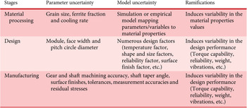
Designing a gearbox is a complex process. The American Gear Manufacturers Association (AGMA) is an important authority responsible for disseminating knowledge pertaining to the design and analysis of gearing. The methods presented by this organisation are in general use in the United States when strength and wear are of primary concern. Although AGMA provides a systematic procedure for designing gears, they also offer numerous correction factors associated with modelling the geometry, materials, manufacturing process and operating conditions. These correction factors have a huge impact on the design. It is critical to accurately ascertain their values to ensure that the gears are safe and reliable but not overdesigned. However, this requires comprehensive knowledge about operating conditions, materials, design and manufacturing processes which are often challenging. The presence of uncertainties involved at various stages of making gearboxes (see Table 2) adds to the challenge of designing safe and reliable gearboxes. The two major decisions in the design of gearboxes are decisions about the dimensions and the material. In addition, a gearbox designer is also expected to fulfil a number of design constraints while also fulfilling multiple functional requirements.
Table 2. Critical review of literature

By relying on the AGMA guidelines and procedure, through a robust design method, we offer an extension on the AGMA design procedure to support robust decision-making for designing gearboxes using coupled decisions that has the following salient features:
-
(i) Consideration of multiple design criteria.
-
(ii) Coupled decision approach for simultaneous material selection and geometry exploration.
-
(iii) Robust decision-making to manage uncertainties.
-
(iv) Consideration of decision coupling for modelling concurrent and hierarchical decisions.
The simplified flowchart to illustrate AGMA procedure (AD) and the proposed robust design method for designing gears (RD) is shown in Figure 1. The design procedure implemented in the two methods can be explained in a simplified way with the following steps:
-
Step 1: Design input. In Step 1, the design inputs required to solve the design problem are identified and defined. The information about power requirement (torque and speed), design variables and their bounds, and constraints are clearly defined.
-
Step 2: Select material. In Step 2, a suitable material is selected. This selection involves making judgments using the information gathered in Step 1. Then, all necessary correction factors as defined by AGMA are applied to the material.
-
Step 3: Determine design variables. In Step 3, suitable values for the design variables are ascertained. This may involve some calculations and iterations.
-
Step 4: Satisfy design constraints. The values ascertained for the design variables and the selected material are checked to determine whether the design constraints identified in Step 1 are satisfied. If the constraints are satisfied, a design solution is obtained, otherwise, Steps 1, 2 and/or 3 are iterated until a satisfactory solution is obtained.
Steps in the AGMA design procedure (AD)
-
Step 1: Design input. In Step 1, design inputs required to solve the design problem are identified and defined. The power requirement (torque and speed), design variables and their bounds, and constraints are clearly defined.
-
Step 2: Coupled DSP. In Step 2, a coupled DSP is formulated. The coupled DSP consists of two decisions defined in Steps 2a and 2b, which are implemented concurrently. Step 2a is a compromise decision, and Step 2b is a selection decision modelled as cDSPs and sDSPs. The implementation of the cDSP helps determine the correct values for design variables, that is, the gear geometry. At the same time, the sDSP is used to select a suitable gear material from a given pool of material alternatives. The two decisions in Figure 1 are used for illustrative purposes, while there could be multiple interacting decisions. In the gearbox example used in this article, there are three interacting decisions. Two coupled decisions of gear design interact with one decision about shaft design (see Section 2).
Uncertainties (A) and Multiple Design Criteria (B) are inputs to the coupled DSP. The control factors, noise factors, responses and bounds are specified for the given design problem for uncertainty management. In the example implemented in this article, three types of uncertainties (Type I, Type II and Type III) are considered (see Tables 3 and 4). For consideration of multiple design criteria, goals are defined and implemented within the coupled DSP construct. By assigning different weights for the multiple goals, several design scenarios are generated.
-
Step 3: Satisfy design constraints. The values ascertained for the design variables and the material selected in Step 2 using coupled DSP are checked to determine whether the design constraints identified in Step 1 are satisfied. If the constraints are satisfied, a design solution is obtained; otherwise, Steps 1 and/or 2 are repeated until a satisfactory solution is obtained.
Steps in the proposed robust design method (RD):

Figure 1. Comparison of proposed design method with American Gear Manufacturers Association (AGMA) for gear design.
Table 3. Uncertainties involved in making of a gearbox

Table 4. Utility of three types of uncertainties in gearbox design

Some distinctive advantages of RD over AD for designing gears are as follows:
-
(i) Exploration of gear design space against multiple conflicting goals,
-
(ii) Simultaneous exploration of gear dimensions against available material alternatives and
-
(iii) Consideration of uncertainties enables the design of reliable and robust gears.
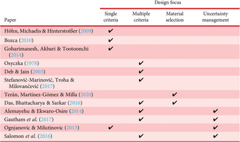
Although mechanical gearboxes are optimised for torque and speed, there are numerous other functional requirements to be satisfied, such as efficiency (Höhn et al. Reference Höhn, Michaelis and Hinterstoißer2009), noise, vibration (Bozca Reference Bozca2010), volume and size (Osyczka Reference Osyczka1978). The available literature that addresses gearbox design as multicriteria design problem. Höhn et al. (Reference Höhn, Michaelis and Hinterstoißer2009), Bozca (Reference Bozca2010) and Goharimanesh et al. (Reference Goharimanesh, Akbari and Tootoonchi2014) present a method for designing gearboxes with a single criterion while Osyczka (Reference Osyczka1978), Deb ' Jain (Reference Deb and Jain2003) and Stefanović-Marinović et al. (Reference Stefanović-Marinović, Troha and Milovančević2017) present a method for designing gearboxes with multiple criteria. Suitable material selection is another critical aspect of designing gearboxes. Multicriteria decision-making methods are common approaches applied in material selection. Terán et al. (Reference Terán, Martínez-Gómez and Milla2020) present multicriteria decision methods for selecting material by optimising surface fatigue in gearbox while also increasing its resistance to wear. Das et al. (Reference Das, Bhattacharya and Sarkar2016) showcase an approach for simultaneous selection of material and geometric variables in gear design using decision-based design. Designing gearboxes in the presence of uncertainty has also received due attention among researchers. Alemayehu ' Ekwaro-Osire (Reference Alemayehu and Ekwaro-Osire2014) offer a probabilistic, multibody dynamic analysis (PMBDA) design approach for designing wind turbine gearboxes by addressing the loading and design parameter uncertainties while considering five performance functions. Gautham et al. (Reference Gautham, Kulkarni, Panchal, Allen and Mistree2017) propose a robust design method for designing gears by addressing the uncertainties associated with the introduction of numerous ‘correction factors’ by the AGMA. The authors introduce a method to eliminate two correction factors from the AGMA design standards for designing a spur gear: the factor of safety in contact and the reliability factor by introducing uncertainty in the magnitude of the load and material properties. On the other hand, Ognjanovic ' Milutinovic (Reference Ognjanovic and Milutinovic2013) adopt a reliability-based methodology to design an automotive gearbox to operate under varying and random operation conditions. Salomon et al. (Reference Salomon, Avigad, Purshouse and Fleming2016) extend the gearbox design optimisation to consider uncertainties in load demand. The authors utilise active robust (AR) optimisation to optimise the number of transmissions and their gearing ratios for an uncertain load demand. AR optimisation is a methodology to design products that attain robustness to uncertain or changing environmental conditions through adaptation.
It has been established that uncertainties degrade a designer’s ability to make an informed decision. When applied, the design decisions do not account for uncertainties induced by noise factors (uncontrollable parameters), design variables (controllable parameters), model approximations used in the simulation models and uncertainty propagation across different length and time scales. Therefore, uncertainty management methods are critical to enable robust decision-making. The body of literature on available robust design methods is discussed by Eifler, Ebro ' Howard (Reference Eifler, Ebro and Howard2013). The robust design method presented in this article is based on the sources of uncertainties. In this article, three types of uncertainty are managed, Types I, II and III. Type I is related to uncertainties due to noise factors; Type II is related to uncertainties due to design variables and Type III is related to uncertainties due to mathematical models. To manage these uncertainties, three robust design methods are utilised, they are, Types I, II and III robust design methods. The details are discussed in Chen et al. (Reference Chen, Allen, Tsui and Mistree1996) and McDowell et al. (Reference McDowell, Panchal, Choi, Seepersad, Allen and Mistree2009). In context of designing gearboxes, uncertainties and methods to deal with the uncertainties are tabulated in Tables 3 and 4, respectively.
In Section 2, we describe the types of decisions required and the interactions among these decisions. In Section 3, the robustness metrics, DCI and EMI, are described in detail. In Section 4, we present the robust formulation for the coupled decision/problem in the context of designing a gearbox. The exploration of the solution space to identify satisficing robust design solutions is covered in Section 5. In Section 5, we present ternary plots as an approach to explore the robust solution space. Finally, we close the article with our remarks in Section 6.
2. Decision coupling
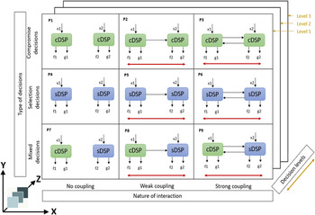
In our previous work, we proposed a classification scheme for coupled decisions using DSPs, called the decision scenario matrix (DSM) (Sharma, Allen ' Mistree Reference Sharma, Allen and Mistree2019). The DSM provides a decision framework for classifying and representing an engineered system as a coupled engineered system with numerous interacting decisions. In this article, we extend the DSM to a MDSM for multilevel hierarchical coupled decisions (see Figure 2). Before making any design exploration or design tradeoff study, the system must be represented as a network of interacting decisions. On one hand, MDSM gives a criteria-governed decision framework for doing so. On the other hand, the MDSM decision framework supports the development of predesigned templates for configuration and execution of decision workflows (Ming et al. Reference Ming, Sharma, Allen and Mistree2019, Reference Ming, Sharma, Allen and Mistree2020).

Figure 2. Multilevel decision scenario matrix (MDSM) (Sharma Reference Sharma2020).
The MDSM is created by identifying and classifying decision scenarios based on three criteria: (i) decision types (selection or compromise), (ii) strength of interaction, and (iii) decision levels. Three axes are used to represent these criteria. The Y-axis represents the type of coupled decisions which may take three forms:
-
(i) Both design decisions involve compromise.
-
(ii) Both design decisions involve selection.
-
(iii) Design decisions involving a combination of selection and compromise.
The X-axis represents the strength of interaction which is coupled through horizontal coupling. Horizontal coupling defines the influence of one DSP over the other at the same level. This also may take three forms:
-
(i) No interaction exists.
-
(ii) Weak or one-way interaction exists.
-
(iii) Strong or two-way interaction exists.
Finally, the Z-axis represents the hierarchy in decisions, and the levels assigned represent the order in which hierarchical decisions must be executed. These levelled decisions are executed in a hierarchy and are coupled to previous decisions made. Level 1 decisions have the highest priority and so on. The decisions at various levels are coupled with adjacent levels defined through vertical coupling. Vertical coupling defines the influence of decisions among adjacent levels.
Defining decision levels and interactions depend on the nature of the design problem and the designers’ judgement. For the design problem presented in the article, the decision levels and interactions considered are shown in Figure 3. Level 1 involves identifying decisions involving gear. Gear decisions involve two decisions that are coupled:
-
(i) The compromise decisions, the gear dimensions.
-
(ii) The selection decision, the gear material.
Gear decisions are coupled to shaft decisions and executed at Level 2. Gear decisions are modelled as coupled selection-compromise DSPs with strong interaction while shaft decisions as compromise DSPs with weak interaction to gear decisions. The weak formulation defines an interaction in which there is one-way flow of information between DSPs. The strong formulation defines an interaction in which there is a two-way flow of information between DSPs. These coupled DSPs are modelled with a robust formulation. The details of the robust formulations are discussed in Section 3. The concise mathematical form for multilevel interaction with strong interactions between DSPs (selection and compromise) on Level 1 and weak interaction between DSPs at two decision levels is shown in Table 5. It is worth noting that system variables (X1) from compromise DSP influence selection goal (MF) in selection DSP and selection alternatives (Y) from selection DSP influence compromise constraints Ai(X1, Y) and goals Gi(X1, Y) in compromise DSP. Further, the compromise goals at Level 1 have influence on the constraints and goals in Level 2. The nature of the information that flows between the DSPs is specific to a particular design problem. In the example presented in this article, information about torque flows from Level 1 to Level 2.

Figure 3. Coupled representation and modelling of gearbox design problem by three interacting decisions.
Table 5. Simplified mathematical form for demonstrating a robust coupled selection – compromise decision using DSPs. The shared variables are in bold type.

3. Robustness formulation
The robust formulation is implemented by incorporating two metrics, the DCI and the EMI, as design goals and constraints. The concept used to measure process capability is extended into design to derive these metrics as the measurements for performance variations caused by manufacturing variations and performance variations corresponding to a range of solutions in a design system are similar (Chen et al. Reference Chen, Simpson, Allen and Mistree1999). However, these design metrics are applicable to the evaluation of design capability when the deviation of design performance cannot be quantified by a statistical distribution as opposed to process capability metrics used to measure performance variations caused by manufacturing variations.
3.1. Design capability index
DCIs represent the safety margin against system failure due to uncertainty in design variables. In particular, DCIs represent the degree of reliability by measuring the capability of design decisions:
-
(i) To satisfy the design requirements.
-
(ii) To tolerate the effect of uncertainty in design variables.
In Figure 4, the mean response (μ y) for the model is illustrated by a solid curve. At x, for the variation of +∆x in a design variable, the expected variation in the response given by the mean response model is ∆Y. This lets us calculate the maximum expected deviation in response for any given value of x and ∆x. In Figure 5, we show the mathematical formulations for implementing DCIs as a goal in DSPs. ‘Smaller is better’ signifies that we are looking to minimise the targeted function, while ‘Larger is better’ signifies maximising the targeted function. Further, ‘Nominal is better’ means we are interested in obtaining a value near to the target set. That is, we want to avoid underachievement as well as overachievement.
-
Step 1: Using a first-order Taylor series expansion, estimate the response variation due to variation in the design variable vector x = {x1, x2, …, xn}. The response variation (∆y) for small variations in design variables is:
(1) $$ \Delta Y=\sum_{i=1}^n\left|\frac{\mathrm{\partial}f}{{\mathrm{\partial}x}_i}\right|\cdot \Delta {x}_i. $$
-
Step 2: Using the mean response (μ y) obtained from the mean response model (f 0(x)) and the response variation due to variation in design variables (ΔY), calculate the DCIs. For a ‘Larger is Better’ case, the DCI is calculated as:
(2)
$$ DCI=\frac{\;{\mu}_y- LRL}{\Delta Y}. $$
Steps for formulating goals as DCIs
The DCI is a mathematical metric representing the safety margin against system failure due to uncertainty in design variables. A DCI < 1 is a mean of the system performance which falls outside the systems requirement range. A DCI ≥ 1 means that the ranged set of design specifications satisfies a ranged set of design requirements, and the system is robust against uncertainty in design variables. Therefore, a designer aims to force DCI to unity so that a more significant portion of performance deviation falls within the design requirements range. The higher the value for DCI, the higher the measure of safety against failure due to uncertainty in design variables (Choi et al. Reference Choi, Austin, Allen, McDowell, Mistree and Benson2005).

Figure 4. Formulation of uncertainty bounds due to variations in a design variable (Choi et al. Reference Choi, Austin, Allen, McDowell, Mistree and Benson2005).

Figure 5. Mathematical constructs for design capability indexes (DCIs).
3.2. Error margin index
EMIs represent the amount of safety margin against system failure due to uncertainty in the design model. In particular, EMIs represent the degree of reliability by measuring the capability of design decisions:
-
(i) To satisfy the design requirements.
-
(ii) To tolerate the effect of uncertainty in design models.
In Figure 6, the model’s mean response (μ y ) is shown as a solid curve, and the two adjacent dotted curves represent the uncertainty bounds associated with the system model. At X, the variation of +∆X in the design variable, the expected variation in the response given by the mean response model is ∆Y. Similarly, for the same change in design variable at X, the expected variation in response for the two uncertainty bounds are ∆Y 1 and ∆Y 2, respectively as shown in Figure 6. This lets us calculate the maximum expected deviation in response for any given value of X and ∆X. In Figure 7, we show the mathematical formulations for implementing EMIs as a goal in DSPs.
-
Step 1: If a system model has k uncertainty bounds, the response variation (∆y j) for each of them for small variation in design variables is calculated as:
(3)where j = 0, 1, 2, …, k (number of uncertainty bounds).
$$ \Delta {y}_j=\sum_{i=1}^n\left|\frac{\mathrm{\partial}{y}_j}{{\mathrm{\partial}x}_i}\right|\cdot \Delta {x}_i, $$
-
Step 2: After evaluating the multiple response variations of mean response function and the k uncertainty bound functions for variations in design variables, the minimum and maximum responses by considering the variability in design variables and uncertainty bounds around the mean response are calculated as:
(4)
$$ {Y}_{max}=\left[(x)+\varDelta {y}_j\right], $$
(5)where j = 0, 1, 2, …, k (number of uncertainty bounds), f 0(x) is the mean response function and f 1(x) …. (x) are the uncertainty bound functions.
$$ {Y}_{min}=\left[(x)-\varDelta {y}_j\right], $$
In Figure 6, we show a mean response function (solid black curve) and two uncertainty bounds (dotted curves in black). At any x, we can calculate the value of maximum (y max ), minimum (y min) and mean response (μ y) arising due to uncertainty bounds. This will let us calculate the maximum expected deviation in response for any given value of x.
-
Step 3: Calculate the upper and lower deviation of response at x as:
(6)
$$ \varDelta {Y}_u={Y}_{max}-(x), $$
(7)
$$ \varDelta {Y}_l=(x)-{Y}_{min}. $$
The deviations ∆y u and ∆y l are shown in Figure 5.
-
Step 4: Using the mean response (μ y) obtained from the mean response model (f 0(x)) and the upper and lower deviations (∆y upper and ∆y lower), the EMIs are calculated as shown in Figure 7. For a ‘Larger is Better’ case, the EMI is calculated:
(8)
$$ EMI=\frac{\mu_y-LRL}{\varDelta {Y}_l}. $$
Steps for formulating goals as EMIs

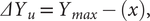
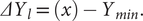

Figure 6. Formulation of uncertainty bounds due to variations in a model (Choi et al. Reference Choi, Austin, Allen, McDowell, Mistree and Benson2005).

Figure 7. Mathematical constructs for EMIs.
The EMI is a mathematical metric representing the safety margin against system failure due to uncertainty in the design models. An EMI < 1 means that a requirement limit may be violated due to uncertainty in the model. An EMI ≥ 1 means that the ranged set of design specifications satisfies a ranged set of design requirements, and the system is robust against uncertainty in design models. Therefore, a designer’s aim is to force EMI to unity so that an uncertainty bound meets a requirement limit. The higher the value for EMI, the higher the measure of safety against failure due to uncertainty in design models (Choi et al. Reference Choi, Austin, Allen, McDowell, Mistree and Benson2005).
4. Coupled DSPs formulation for robust exploration of gearbox decisions
We are required to design a one-stage reduction gearbox consisting of a gear-pinion arrangement and shafts, one each at the input and output end of the gear-pinion pair. Broadly, our task is to recommend the dimensions and material for the design. The design decisions are to be taken considering the following design requirements:
-
(i) Satisficing solutions against multiple conflicting goals.
-
(ii) The influence of gear-pinion design on shaft design and vice versa.
-
(iii) The influence of selected material on dimensions and vice versa.
-
(iv) The expected variability in design variables, and materials including a method to manage the effect of such variability to effect robust decision-making.
4.1. Problem statement
The design of a one-stage reduction gearbox (see Figure 8) with a gear ratio of 4 is required. The torque at input is at least 80 Nm @ 3500 rpm. The gears are required to endure at least 107 fatigue cycles. The gears are cut using a rack cutter arrangement with pressure angle (α) = 20°. The reliability for gears must be at least 99%. The gearbox is to be designed for a uniform power source and moderate shock in loads. Restrictions regarding the maximum allowable stresses on the gears and shafts are specified. The design quality is measured in terms of design goals that are to be achieved as much as possible. Specifically, we need a design that has low weight and smaller height while achieving maximum torque. However, the design must have a robust performance to minimise the impact of uncertainties associated with design variables and material properties on performance. The task is to select gear material from a given pool of materials and dimensions for gears and to recommend shear strength for shaft material and shaft dimensions that give a robust performance with respect to the constraints and the design quality specified. The material properties for shafts are available for selection within the specified bounds, while gear materials are available for selection.

Figure 8. Schematic of a one-stage reduction gearbox.
4.2. Mathematical derivation for converting gearbox design goals into robust design goals
Three goals are formulated as DCIs, these are, weight of gear pair (Wg), size of gearbox (H) and weight of shaft (Ws). One goal is formulated as an EMI goal, that is, Torque. The mathematical derivation for the four compromise goals (three goals for gear design and one goal for shafts design) as robustness goals are shown in Equations (9)–(44) using Equations (1)–(8).
Goal 2: Weight of gear pair (Wg):
 $$ {W}_g=13.35(\rho \cdot b\cdot {m}^2\cdot {z}^2)\times {10}^{-9}(\mathrm{k}\mathrm{g}), $$
 $$ \frac{\mathrm{\partial}{W}_g}{\mathrm{\partial}b}=13.35(\unicode{x03C1} \cdot {\mathrm{m}}^2\cdot {z}^2)\times {10}^{-9}, $$
 $$ \frac{\mathrm{\partial}{W}_g}{\mathrm{\partial}m}=26.7(\rho \cdot b\cdot m\cdot {z}^2)\times {10}^{-9}, $$
 $$ \frac{\mathrm{\partial}{\mathrm{W}}_{\mathrm{g}}}{\mathrm{\partial}z}=26.7(\rho \cdot b\cdot {m}^2\cdot z)\times {10}^{-9}, $$
 $$ \Delta {W}_g=\left|\frac{\mathrm{\partial}{W}_g}{\mathrm{\partial}b}\right|\cdot \varDelta b+\left|\frac{\mathrm{\partial}{W}_g}{\mathrm{\partial}m}\right|\cdot \varDelta m+\left|\frac{\mathrm{\partial}{W}_g}{\mathrm{\partial}z}\right|\cdot \varDelta z, $$
 $$ \Delta {W}_g=13.35(\rho \cdot m\cdot z)[(m\cdot \varDelta b)+2(b\cdot z\cdot \varDelta m)+2(b\cdot m\cdot \varDelta z)]\times {10}^{-9}, $$
 $$ DCIWg=\frac{\;{URL}_{Wg}-{W}_g\;}{\Delta {W}_g}, $$
 $$ DCIWg=\frac{URL_{Wg}-13.35(\rho \cdot b\cdot {m}^2\cdot {z}^2)\times {10}^{-9}}{13.35(\rho \cdot m\cdot z)[(m\cdot z\cdot \varDelta b)+2(b\cdot z\cdot \varDelta m)+2(b\cdot m\cdot \varDelta z)]\times {10}^{-9}}, $$
 $$ \Delta H=\left|\frac{\mathrm{\partial}H}{\mathrm{\partial}m}\right|\cdot \varDelta m+\left|\frac{\mathrm{\partial}H}{\mathrm{\partial}z}\right|\cdot \varDelta z, $$
 $$ \Delta H=5[(z\cdot \varDelta m)+(m\cdot \varDelta z)]. $$
Goal 3: Size of gearbox (H):
 $$ H=5m\cdot z(\mathrm{m}\mathrm{m}), $$
 $$ \frac{\partial H}{\partial m}=5z, $$
 $$ \frac{\partial H}{\partial z}=5m, $$
 $$ DCIH=\frac{\;{URL}_H-H\;}{\Delta H}, $$
 $$ DCIH=\frac{URL_H-5mz}{5[(z\cdot \Delta m)+(m\cdot \Delta z)]}. $$
Goal 5: Weight of shaft (Ws):
 $$ {W}_s=6.129\left({D}_i^2+{D}_o^2\right)\times {10}^{-3}\;\left(\mathrm{kg}\right), $$
 $$ \frac{\partial {W}_s}{\partial {D}_i}=12.26{D}_i\times {10}^{-3}, $$
 $$ \frac{\partial {W}_s}{\partial {D}_o}=12.26{D}_o\times {10}^{-3}, $$
 $$ \Delta {W}_s=\left|\frac{\mathrm{\partial}{W}_s}{\mathrm{\partial}{D}_i}\right|\cdot \varDelta {D}_i+\left|\frac{\mathrm{\partial}{W}_s}{\mathrm{\partial}{D}_o}\right|\cdot \varDelta {D}_o, $$
 $$ \Delta {W}_s=12.26[({D}_i\cdot \varDelta {D}_i)+({D}_o\cdot \varDelta {D}_o)]\times {10}^{-3}, $$
 $$ DCIWs=\frac{\;{URL}_{Ws}-{W}_s\;}{\Delta {W}_s}, $$
 $$ DCIWs=\frac{URL_{Ws}-6.129({D}_i^2+{D}_o^2)\times {10}^{-3}}{12.26[({D}_i\cdot \varDelta {D}_i)+({D}_o\cdot \varDelta {D}_o)\times {10}^{-3}}. $$
Goal 4: Torque (Tu and Tm):
 $$ {T}_u={\left(\frac{S_c}{18,348}\right)}^2(b\cdot {m}^2\cdot {z}^2)(\mathrm{N}\mathrm{m}), $$
 $$ {T}_m=\left(\frac{S_t}{10,760}\right)(b\cdot {m}^2\cdot z)(\mathrm{N}\mathrm{m}), $$
 $$ \frac{\mathrm{\partial}{T}_u}{\mathrm{\partial}b}={\left(\frac{S_c}{18,348}\right)}^2({m}^2\cdot {z}^2), $$
 $$ \frac{\mathrm{\partial}{T}_u}{\mathrm{\partial}m}={\left(\frac{S_c}{18,348}\right)}^2(2\cdot b\cdot m\cdot {z}^2), $$
 $$ \frac{\mathrm{\partial}{T}_u}{\mathrm{\partial}z}={\left(\frac{S_c}{18,348}\right)}^2(2\cdot b\cdot {m}^2\cdot z), $$
 $$ \Delta {T}_u=\left|\frac{\mathrm{\partial}{T}_u}{\mathrm{\partial}b}\right|\cdot \varDelta b+\left|\frac{\mathrm{\partial}{T}_u}{\mathrm{\partial}m}\right|\cdot \varDelta m+\left|\frac{\mathrm{\partial}{T}_u}{\mathrm{\partial}z}\right|\cdot \varDelta z, $$
 $$ \Delta {T}_u={\left(\frac{S_c}{11,612}\right)}^2(m\cdot z)[(m\cdot z\cdot \varDelta b)+2(b\cdot z\cdot \varDelta m)+2(b\cdot m\cdot \varDelta z)], $$
 $$ {T}_{max}={T}_u+\Delta {T}_u, $$
 $$ {T}_{max}={(\frac{S_c}{18,348})}^2(m\cdot z)[(b\cdot m\cdot z)+(m\cdot z\cdot \varDelta b)+2(b\cdot z\cdot \varDelta m)+(2b\cdot m\cdot \varDelta z)], $$
 $$ \Delta {T}_u={T}_{max}-{T}_m, $$
 $$ {\displaystyle \begin{array}{l}\Delta Tupper={\left(\frac{S_c}{\mathrm{18,348}}\right)}^2\left(m\bullet z\right)\\ {}\;[(b\bullet m\bullet z\Big)+\left(m\bullet z\bullet \varDelta b\right)+2\left(b\bullet z\bullet \varDelta m\right)+2(b\bullet m\bullet \varDelta z)]-\left(\frac{S_t}{\mathrm{10,760}}\right)\left(b\bullet {m}^2\bullet z\right),\end{array}} $$
 $$ EMIT=\frac{\mu_y-LRL}{\varDelta {Y}_l}=\frac{T_m-{LRL}_T}{\Delta {T}_u}, $$
 $$ EMIT=\frac{(\frac{S_t}{10,760})(b\cdot {m}^2\cdot z)-{LRL}_T}{\Delta {T}_u}, $$
 $$ EMIT=\frac{\left(\frac{S_t}{10,760}\right)(b\cdot {m}^2\cdot z)-{LRL}_T}{{(\frac{S_c}{18,348})}^2m\cdot z(b\cdot m\cdot z+m\cdot z\cdot \varDelta b+2b\cdot z\cdot \varDelta m+2b\cdot m\cdot \varDelta z)-\left(\frac{S_t}{10,760}\right)b\cdot {m}^2\cdot z}. $$
Following the steps outlined in Figure 1, Table 6 is formulated. The information in Table 6 is defined using four keywords: Given, Find, Satisfy and Minimise. The keyword ‘Given’ contains the design input, while ‘Find’ defines the coupled decisions. The determination of compromise decisions (gearbox dimensions) and selection decision (gear material) forms a coupled decision. The selection decision involves the process of choosing among a number of possibilities considering several measures of merit or attributes, while compromise decision involves the determination of the ‘right’ values (or combination) of design variables (or parameters). Compromise and selection decisions are respectively modelled with a cDSP and sDSP. The solution to the coupled cDSP–sDSP is explored by considering multiple design criteria and uncertainties. The multiple design criteria are defined by goals G1 to G5. The uncertainty is managed by modifying the original design goals into robustness metrics (see Equations (9)–(44)). The keyword ‘Minimise’ specifies iterating until a satisfactory result is obtained. A satisfactory result is obtained when the constraints are satisfied, and the deviations from the predefined design targets are minimised. The mathematical foundation for designing a gearbox is available in Budynas ' Nisbett (Reference Budynas and Nisbett2008). The mathematical derivation for the four compromise goals (three goals for gear design and one goal for shaft design) as robustness goals are shown in Equations (9)–(44) and summarised in Table 6. Further information about this formulation is available in the work of Sharma (Reference Sharma2020).
Table 6. Mathematical formulation for robust design of a gearbox (Additional information about variables is available in the Nomenclarure section at the end of the article.)

5. Results and discussion
How are ternary plots created for solution space exploration?
A ternary plot is drawn using a triangle, as shown in Figure 9. Each side of the triangle represents a goal. In a ternary plot, the values of the three goals usually, this constant is represented as 1.0 or 100%. For solution space exploration, the value of K = 1, and each side represents the weights assigned to the goal. Every point on a ternary plot represents a different combination of weights for the goals. The interior colour coding indicates the value achieved for a goal when a specific combination of weights is assigned to the three goals. In Figure 9, the different colours in the triangle’s interior indicate the values achieved for a particular goal when different combinations of weights to the three goals are assigned. Similarly, plots are drawn for the other remaining goals. In each plot, an acceptable region for the particular goal is identified. Finally, a superimposed plot is made to ascertain the region of overlap, that is, the region where all goals are met simultaneously.

Figure 9. Ternary plot for solution space exploration.
The Decision Scenario is solved for 11 different design scenarios. These scenarios are selected based on a designer’s desire to capture the design space to explore the solution space using different combinations of goal weights. Different weights are assigned to different goals indicating a designer’s interest in achieving the goal targets. Assigning 1 (Scenarios 1–3) to a goal means that a designer’s interest is to achieve the goal target as closely as possible while ignoring the other goals. For instance, assigning weight w 1 = 1 to weight would mean that the designer wants to obtain the weight target as closely as possible while not considering the other two goals. Assigning 0.5 (Scenarios 4–6) to 2 goals means that the designer is equally interested in achieving the target of the two goals while not considering the third goal. With the design solutions obtained in different design scenarios, ternary plots for each goal are drawn. The axes of the ternary plots are the weights assigned to each goal and the coloured ternary space in the interior indicate the achieved value of that specific goal. For example, the ternary plot for the weight goal shows the value achieved for the weight goal within the ternary space when different weights are assigned to the other goals. For the design example presented in this article, the three goals of the compromise DSP at Level 1 (DCIWg, DCIH and EMIT) are shown in ternary plots. Then an acceptable region within each ternary plot is identified. Consequently, the acceptable regions identified from each ternary plot are superimposed in one plot to determine feasible solution regions considering these three goals. Finally, the coupled solutions, that are, gear material (sDSP at Level 1) and shaft decision (cDSP at Level 2) when the three gear goals (cDSP at Level 1) are satisfied, are obtained.
For the DCIWg goal (G2 in Table 6), our interest lies in identifying robust solutions, that is, a higher value for DCIWg. The solution space in Figure 10 is composed of robust solutions for gear weight ensuring robustness against parameter uncertainty. The red region contains the robust solutions that achieve the maximum value for the DCIWg goal whereas the blue region contains the robust solutions that achieves the minimum value for DCIWg goal. The maximum attained value for DCIWg goal is 40.82 while the minimum attained value is 18.69. An acceptable region within the solution space is defined as DCIWg ≥ 22 and is identified by the black dashed line. All solution points within this region are acceptable as they satisfy the requirement for gear weight under parameter uncertainty.

Figure 10. Solution space for the weight goal when various weights are assigned to the other goals.
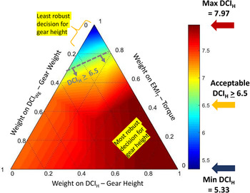
For the DCIH goal (G3 in Table 6), our interest lies in identifying robust solutions with a higher value for DCIH. The solution space in Figure 11 is composed of robust solutions for gear height, ensuring robustness against parameter uncertainty. The red region contains the robust solutions that achieve the maximum value for the DCIH goal. In contrast, the blue region contains the robust solutions that achieve the minimum value for the DCIH goal. The maximum attained value for the DCIH goal is 7.97, while the minimum attained value is 5.33. An acceptable region within the solution space is defined as DCIH ≥ 6.5 and is identified by the grey dashed line. All solution points lying within this region are acceptable as they satisfy the requirement for gear height under parameter uncertainty.

Figure 11. Solution space for size when various weights are assigned to the other goals.
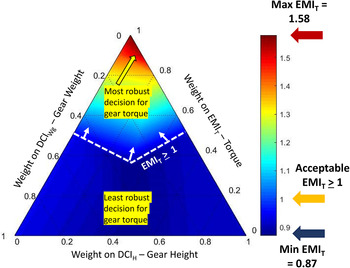
For the EMIT goal (G4 in Table 6), our interest lies in identifying robust solutions, that is, those with higher values of EMIT. The solution space in Figure 12 is composed of robust solutions for gear torque, ensuring robustness against model and parameter uncertainty. The red region contains the robust solutions that achieve maximum values for the EMIT goal. The blue region contains the robust solutions that achieve the minimum value for the EMIT goal. The maximum attained value for the EMIT goal is 1.58, while the minimum value attained is 0.87. An acceptable region within the solution space has EMIT ≥ 1 and is delineated by the white dashed line. All solution points lying within this region are acceptable as they satisfy the requirement for gear torque under both model and parameter uncertainty.

Figure 12. Solution space for torque when various weights are assigned to the other goals.
As our interest lies in identifying a satisficing robust solution region against multiple conflicting goals, we derive a superimposed robust solution space as discussed earlier and shown in Figure 13. The overlapping region in Figure 13 is the search space for identifying robust design solutions that meet the conflicting needs of minimising gear weight and height while maximising gear torque. One design scenario (Scenario 10) lies within the overlap region. The design variables corresponding to this design solution are shown in Table 7.

Figure 13. Superimposed satisficing solution space.
Table 7. Coupled gear decisions – robust exploration

Note: X 1 = AISI 1018.
Level 1 decisions (coupled cDSP–sDSP shown in Table 7) pertaining to gear decisions are vertically coupled to Level 2 (shaft decisions). The functional coupling occurs because the shaft torque transmission capability must match the torque transmission capability for which the gears are designed. After selecting the design solution for the gear, the design variables for shafts that are compatible with the gear are selected. The design variables for the shaft in Scenario S10 (see Table 8) is the shaft design corresponding to the gear designed.
Table 8. Coupled gear shaft decisions – robust exploration

6. Closure
Uncertainties and decision coupling are prevalent in connected systems. Therefore, addressing uncertainties and decision interactions is critical for designing connected systems. In this article, a method for robust design using coupled decisions to support decision-making of design decisions in a coupled decision environment while managing the uncertainties involved is presented. Two major gaps are identified, (Gap 1) the method to design using coupled decisions and (Gap 2) the method to manage uncertainties in a coupled decision environment. Gap 1 is addressed by developing criteria to couple and model interacting decisions using DSPs (see Section 2). Gap 2 is addressed by incorporating robustness metrics (DCI/ EMI) as goals and constraints in coupled DSPs (see Section 3). Decision coupling is modelled by introducing the concept of vertical coupling and horizontal coupling. Through horizontal coupling, concurrent decisions are modelled and through vertical coupling, hierarchical decisions are modelled. To manage uncertainties, the robustness metric (DCI) is incorporated as design goals and constraints. The decision interaction and uncertainty management is implemented using a cDSP construct. The example involving the design of a one-stage reduction gearbox is used to demonstrate the robust design method.
To improve the quality and reliability of design decisions, we assert that it is critical to consider the coupling in decisions and simultaneously manage uncertainties about design decisions. By accounting for coupling in decisions, we expand our search space with the possibility of finding higher quality design solutions. By managing uncertainties, we improve the validity and usefulness of the undertaken decisions, therefore, improving the quality and reliability of the design by producing design solutions whose performance are insensitive to different sources of uncertainties. The proposed robust design method is illustrated through an example involving the design of a one-stage reduction gearbox. The proposed method is generalisable to engineering design problems, especially when there is dependence among the design decisions and prevalent uncertainties in such decisions are likely to invalidate the design solutions. Our approach is to determine the compromise among design requirements that is most effective at increasing the overall performance. However, it is critical to explore different robustness management strategies (Sigurdarson, Eifler ' Ebro Reference Sigurdarson, Eifler and Ebro2019) that may be more suitable for considering robustness and/or optimality. To sum up, our contribution in this article is a method for robust design when the design decisions are coupled.
Acknowledgements
G.S. acknowledges financial support from the Center for Advanced Vehicular Systems at the Mississippi State University, Starkville. He is thankful to his academic mentors, J.K.A. and F.M., who supported him financially from the John and Mary Moore Chair and the L.A. Comp Chair at the University of Oklahoma, Norman.
Nomenclature
- b
-
gear face width
- cDSP
-
compromise decision support problem
- D i
-
input shaft diameter
- D o
-
output shaft diameter
- DCI
-
design capability index
- EMI
-
error margin index
- Ij
-
relative importance of attribute j
- LRL
-
lower requirement limit
- m
-
gear module
- MDSM
-
multilevel decision scenario matrix
- MFi
-
merit function for alternative i
- Rij
-
normalised rating of alternative i for attribute j
- S c
-
maximum allowable contact stress
- S t
-
maximum allowable bending stress
- sDSP
-
selection decision support problem
- T m
-
mean function for torque
- T u
-
upper limit function for torque
- URL
-
upper requirement limit
- z
-
number of teeth in input gear
- ρ
-
density of gear material
Glossary
- Compromise decision
-
The decision requires the ‘right’ values (or combination) of design variables (or parameters) to be determined.
- Design capability index (DCI)
-
A mathematical metric that represents the safety margin against system failure due to uncertainty in design variables.
- Error margin index (EMI)
-
A mathematical metric that represents the safety margin against system failure due to uncertainty in the design models.
- Selection decision
-
The process of choosing among possibilities considering several measures of merit or attributes.
- Type I robust design
-
Type I robust design is used to identify values of a control factor (design variable) that satisfy a set of performance requirements despite variations in noise factors.
- Type II robust design
-
Type II robust design is used to identify values of a control factor (design variable) that satisfy a set of performance requirements despite variations in control factors themselves.
- Type III robust design
-
Type III robust design is used to obtain design solutions that are insensitive to variability or uncertainty embedded within the model that defines the relationship among design variables and response.


 Open access