


Impact Statement
This paper presents DL4DS the first open-source library with state-of-the-art and novel deep learning algorithms for empirical downscaling.
1. Introduction
Downscaling aims to bridge the gap between the large spatial scales represented by global climate models (GCMs) to the smaller scales required for assessing regional climate change and its impacts (Maraun and Widmann, Reference Maraun and Widmann2017). This task can be approached via dynamical or statistical downscaling. In the former, a high-resolution regional climate model is nested into a GCM over the domain of interest (Rummukainen, Reference Rummukainen2010), while the latter aims to learn empirical links between the large- and local-scale climate that are in turn applied to low-resolution climate model output. Statistical or empirical downscaling comes with the benefit of a lower computational cost compared to its dynamical counterpart.
Machine learning (ML) can be defined as the study of computer algorithms that improve automatically by finding statistical structure (building a model) from training data for automating a given task. The field of ML started to flourish in the 1990s and has quickly become the most popular and most successful subfield of artificial intelligence (AI) thanks to the availability of faster hardware and larger training datasets. Deep learning (DL; Bengio et al., Reference Bengio, Lecun and Hinton2021) is a specific subfield of ML aimed at learning representations from data putting emphasis on learning successive layers of increasingly meaningful representations (Chollet, Reference Chollet2021). DL has shown potential in a wide variety of problems in Earth Sciences dealing with high-dimensional and complex data and offers exciting new opportunities for expanding our knowledge about the Earth system (Huntingford et al., Reference Huntingford, Jeffers, Bonsall, Christensen, Lees and Yang2019; Reichstein et al., Reference Reichstein, Camps-Valls, Stevens, Jung, Denzler, Carvalhais and Prabhat2019; Dewitte et al., Reference Dewitte, Cornelis, Müller and Munteanu2021; Irrgang et al., Reference Irrgang, Boers, Sonnewald, Barnes, Kadow, Staneva and Saynisch-Wagner2021).
The layered representations in DL are learned via models called neural networks, where an input n-dimensional tensor is received and multiplied with a weights tensor to produce an output. A bias term is usually added to this output before passing the result through an element-wise nonlinear function (also called activation). Convolutional neural networks (CNNs; LeCun et al., Reference LeCun, Boser, Denker, Henderson, Howard, Hubbard and Jackel1989) are a type of neural network that rely on the convolution operation, a linear transformation that takes advantage of the implicit structure of gridded data. The convolution operation uses a weight tensor that operates in a sliding window fashion on the data, meaning that only a few input grid points contribute to a given output and that the weights are reused since they are applied to multiple locations in the input. CNNs have been used almost universally for the past few years in computer vision applications, such as object detection, semantic segmentation and super-resolution. CNNs show performances on par with more recent models such as visual Transformers (Liu et al., Reference Liu, Mao, Wu, Feichtenhofer, Darrell and Xie2022) while being more efficient in terms of memory and computations.
In spite of recent efforts in the computer science community, the field of DL still lacks solid mathematical foundations. It remains fundamentally an engineering discipline heavily reliant on experimentation, empirical findings and software developments. While scientific software tools such as Numpy (Harris et al., Reference Harris, Millman, van der Walt, Gommers, Virtanen, Cournapeau, Wieser, Taylor, Berg, Smith, Kern, Picus, Hoyer, van Kerkwijk, Brett, Haldane, del Ro, Wiebe, Peterson, Gérard-Marchant, Sheppard, Reddy, Weckesser, Abbasi, Gohlke and Oliphant2020), Xarray (Hamman and Hoyer, Reference Hamman and Hoyer2017), or Jupyter (Kluyver et al., Reference Kluyver, Ragan-Kelley, Pérez, Granger, Bussonnier, Frederic, Kelley, Hamrick, Grout, Corlay, Ivanov, Avila, Abdalla, Willing, Loizides and Schmidt2016) have an essential role in modern Earth Sciences research workflows, state-of-the-art domain-specific DL-based algorithms are usually developed as proof-of-concept scripts. For DL to fulfill its potential to advance Earth Sciences, the development of AI- and DL-powered scientific software must be carried out in a collaborative and robust way following open-source and modern software development principles.
2. CNN-Based Super-Resolution for Statistical Downscaling
Statistical downscaling of gridded climate variables is a task closely related to that of super-resolution in computer vision, considering that both aim to learn a mapping between low-resolution and high-resolution grids (Wang et al., Reference Wang, Chen and Hoi2021). Unsurprisingly, several DL-based approaches have been proposed for statistical or empirical downscaling of climate data in recent years (Vandal et al., Reference Vandal, Kodra, Ganguly, Michaelis, Nemani and Ganguly2017; Höhlein et al., Reference Höhlein, Kern, Hewson and Westermann2020; Leinonen et al., Reference Leinonen, Nerini and Berne2020; Liu et al., Reference Liu, Ganguly and Dy2020; Stengel et al., Reference Stengel, Glaws, Hettinger and King2020; Harilal et al., Reference Harilal, Singh and Bhatia2021). Most of these methods have in common the use of convolutions for the exploitation of multivariate spatial or spatiotemporal gridded data, that is 3D (height/latitude, width/longitude, channel/variable) or 4D (time, height/latitude, width/longitude, and channel/variable) tensors. Therefore, CNNs are efficient at leveraging the high-resolution signal from heterogeneous observational datasets, from now on called predictors or auxiliary variables, while downscaling low-resolution climatological fields.
In our search for efficient architectures for empirical downscaling, we have developed DL4DS, a library that draws from recent developments in the field of computer vision for tasks such as image-to-image translation and super-resolution. DL4DS is implemented in Tensorflow/Keras, a popular DL framework, and contains a collection of building blocks that abstract and modularize a few key design strategies for composing and training empirical downscaling DL models. These strategies are discussed in the following section.
3. DL4DS Core Design Principles and Building Blocks
The core design principles and general architecture of DL4DS are discussed in the following subsections. An overall architecture of DL4DS is shown in Figure 1, while some of the building blocks and network architectures are shown in Figures 2 and 3.
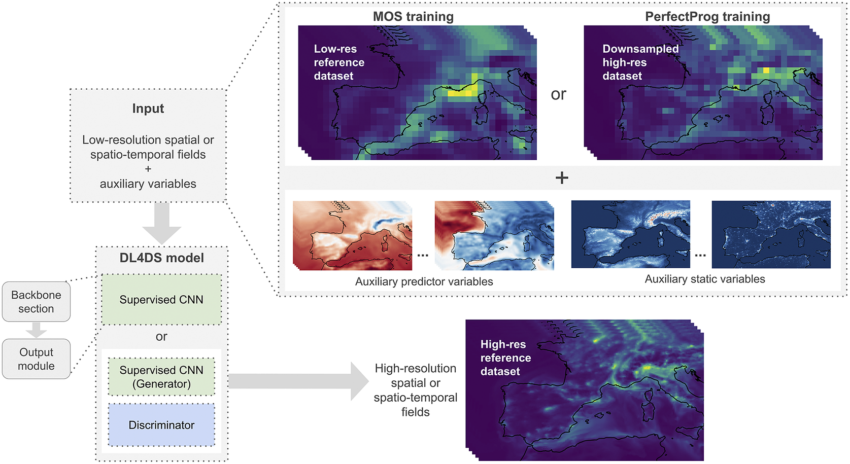
Figure 1. General architecture of DL4DS. A low-resolution gridded dataset can be downscaled, with the help of auxiliary predictor and static variables, and a high-resolution reference dataset. The mapping between the low- and high-resolution data is learned with either a supervised or a conditional generative adversarial DL model.
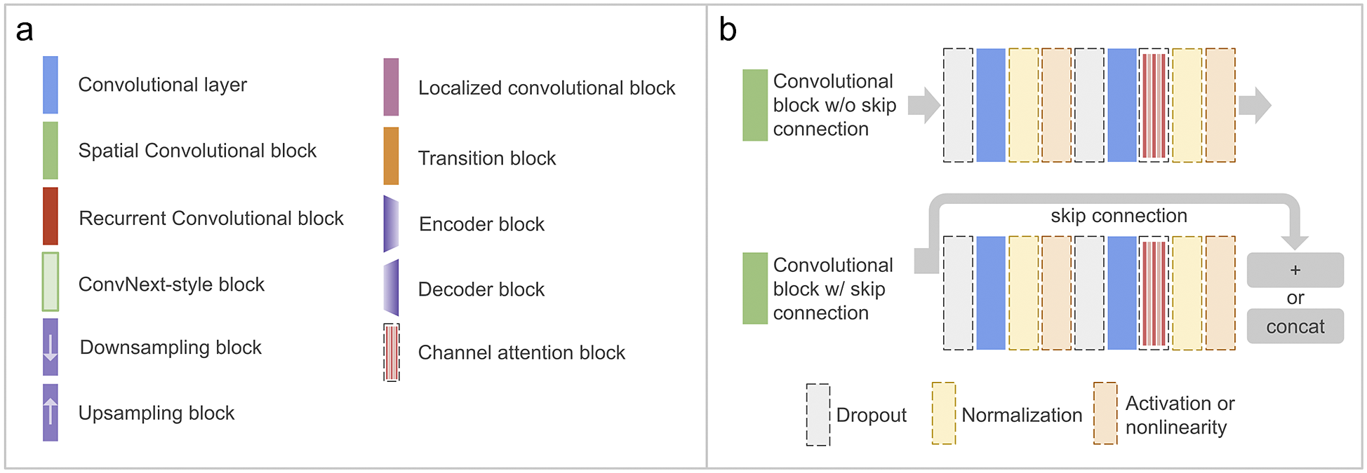
Figure 2. Panel (a) shows the main blocks and layers implemented in DL4DS. Panel (b) shows the structure of the main spatial convolutional block, a succession of two convolutional layers with interleaved regularization operations, such as dropout or normalization. Blocks and operations shown with dashed lines are optional.
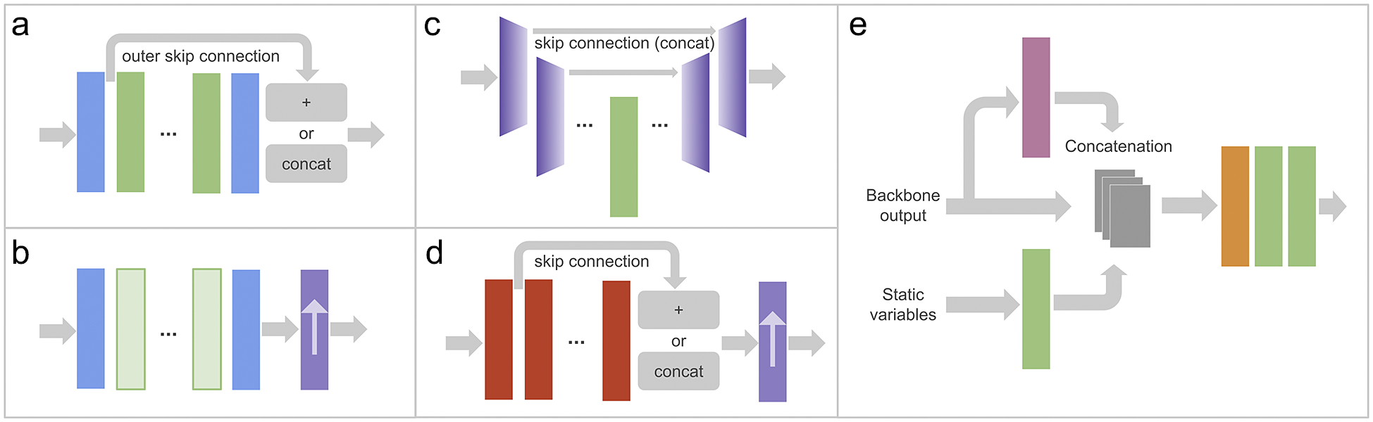
Figure 3. DL4DS supervised DL models, as well as generators, are composed of a backbone section (examples in panels [a–d]) and an output module (panel [e]). Panel (a) shows the backbone of models for downscaling pre-upsampled spatial samples using either residual or dense blocks. Panel (b) presents the backbone of a model for downscaling spatial samples using ConvNext-like blocks and one of the post-upsampling blocks described in Section 3.4.1. Panel (c) shows the backbone of a model for downscaling pre-upsampled spatial samples using an encoder-decoder structure. Panel (d) shows the backbone of a model for downscaling spatiotemporal samples using recurrent-convolutional blocks and a post-upsampling block. These backbones are followed by the output module (see Section 3.4.2) shown in panel (e). The color legend for the blocks used here is shown in Figure 2a.
3.1. Type of statistical downscaling
Statistical downscaling methods aim to derive empirical relationships between an observed high-resolution variable or predictand and low-resolution predictor variables (Maraun and Widmann, Reference Maraun and Widmann2017). Two main types of statistical downscaling can be defined depending on the origin of the predictors used for training; Model output statistics (MOS), where the predictors are taken directly from GCM outputs, and Perfect Prognosis (PerfectProg) methods, that relies on observational datasets for both predictand and predictors (see Figure 1). Most of the DL-based downscaling methods proposed to date, work in PerfectProg setup, where a high-resolution observational dataset is used to create paired training samples via a downsampling or coarsening operation (Vandal et al., Reference Vandal, Kodra, Ganguly, Michaelis, Nemani and Ganguly2017; Leinonen et al., Reference Leinonen, Nerini and Berne2020; Stengel et al., Reference Stengel, Glaws, Hettinger and King2020). The trained model is then applied to the desired, unseen during training, low-resolution data in a domain-transfer fashion. Other approaches such as those proposed by Höhlein et al. (Reference Höhlein, Kern, Hewson and Westermann2020) or Harilal et al. (Reference Harilal, Singh and Bhatia2021), model a cross-scale transfer function between explicit low-resolution and high-resolution datasets. DL4DS supports both training frameworks, with explicitly paired samples (in MOS fashion) or with paired samples simulated from high-resolution fields (in PerfectProg fashion).
3.2. Multivariate modeling and auxiliary variables
Using high-resolution static predictors fields, such as, topography, distance from the sea, and land-sea mask, as well as high- or intermediate-resolution essential climate variables, can help improve the inference capacity of empirical downscaling methods (Maraun and Widmann, Reference Maraun and Widmann2017; Vandal et al., Reference Vandal, Kodra, Ganguly, Michaelis, Nemani and Ganguly2017; Höhlein et al., Reference Höhlein, Kern, Hewson and Westermann2020). The most straightforward way to include these additional predictors and static variables is to merge (concatenate) them across the channel dimension with the input low-resolution fields. DL4DS can handle an arbitrary number of time-varying high- or intermediate-resolution predictors and high-resolution static variables. Additionally, static high-resolution fields are passed through a convolutional block in the output module as shown in Figure 3e in order to emphasize high-resolution topographic information.
3.3. Preprocessing and normalization
DL4DS implements a couple of preprocessing methods aimed at normalizing or standardizing multi-dimensional gridded datasets, a required step when splitting the data into train and validation/test sets used for training and testing DL models. These procedures, namely mix-max and standardization scalers, are implemented as classes (dl4ds.MinMaxScaler and dl4ds.StandardScaler) in the preprocessing module of DL4DS. These classes extend the functionality of methods from the Scikit-learn package (Pedregosa et al., Reference Pedregosa, Varoquaux, Gramfort, Michel, Thirion, Grisel, Blondel, Prettenhofer, Weiss, Dubourg, Vanderplas, Passos, Cournapeau, Brucher, Perrot and Duchesnay2011) aimed at scaling tabular or 2D data. DL4DS scalers can handle 3D and 4D datasets with NaN values in either numpy.ndarray or xarray.Dataarray formats.
3.4. Architecture of the super-resolution models in DL4DS
The super-resolution networks implemented in DL4DS aim at learning a mapping from low or coarse-resolution to high-resolution grids. The super-resolution networks in DL4DS are composed of two main parts, a backbone section, and an output module, as depicted in Figure 1.
3.4.1. Backbone section
We adopt several strategies for the design of the backbone sections, as shown in Figure 3a–d. The main difference is the particular arrangement of convolutional layers. In DL4DS, the backbone type can be set with the backbone parameter of the training classes mentioned in Section 3.4.1:
-
• Convnet backbone—Composed of standard convolutional blocks. As shown in Figure 2b, each spatial convolutional block is composed of two convolutional layers (using 3 × 3 kernels) with some interleaved optional operations, such as dropout (Srivastava et al., Reference Srivastava, Hinton, Krizhevsky, Sutskever and Salakhutdinov2014), batch/layer normalization or a channel attention block (discussed in Section 3.4.1).
-
• Resnet backbone—Composed of residual blocks or convolutional blocks with skip connectionsFootnote 1 that learn residual functions with reference to the layer inputs. Residual skip connections have been widely employed in super-resolution models (Wang et al., Reference Wang, Chen and Hoi2021) in the past. In DL4DS, we implemented cross-layer skip connections within each residual block and outer skip connections at the backbone section level (He et al., Reference He, Zhang, Ren and Sun2016).
-
• Densenet backbone—Composed of dense blocks (see Figure 2b). As in the case of the Resnet backbone, we implement cross-layer skip connections within each dense block and outer skip connections at the backbone section level (Huang et al., Reference Huang, Liu, Maaten and Weinberger2017).
-
• Unet backbone—Inspired by the structure of the U-Net DL model (Ronneberger et al., Reference Ronneberger, Fischer, Brox, Navab, Hornegger, Wells and Frangi2015), this backbone is composed of encoder and decoder blocks with skip connections, as depicted in Figure 3c. The encoder block consists of a convolutional block plus downsampling via max pooling,Footnote 2 while the decoder block consists of upsampling, concatenation with skip feature channelsFootnote 3 from the encoder section, followed by a convolutional block. This backbone is only implemented for pre-upsampled spatial samples.
-
• Convnext backbone—Based on the recently proposed ConvNext model (Liu et al., Reference Liu, Mao, Wu, Feichtenhofer, Darrell and Xie2022), we implemented a backbone with depth-wise convolutional layers and larger kernel sizes (7x7). To the best of our knowledge, this is the first time that a ConvNext-style block architecture has been applied to the task of statistical downscaling.
3.4.1.1. Spatial and spatiotemporal modeling
While CNNs excel at modelling spatial or gridded data, hybrid convolutional and recurrent architectures are designed to exploit spatiotemporal sequences. Convolutional Long Short-Term Memory (ConvLSTM, Shi et al., Reference Shi, Chen, Wang, Yeung, Wong and Woo2015) and convolutional Gated-Recurrent-Units (Ballas et al., Reference Ballas, Yao, Pal and Courville2015) are examples of models that have been used for downscaling time-evolving gridded data (Leinonen et al., Reference Leinonen, Nerini and Berne2020; Harilal et al., Reference Harilal, Singh and Bhatia2021). DL4DS can model either spatial or spatiotemporal data, by either using standard convolutional blocks or recurrent convolutional blocks. The spatiotemporal network in Figure 3d contains recurrent convolutional blocks to handle 4D training samples (with time dimension). The structure of these recurrent convolutional blocks is similar to that of the main convolutional block shown in Figure 2b but using convolutional LSTM layers instead of standard convolutional ones.
3.4.1.2. Channel attention
In DL4DS, we implement a channel attention mechanism based on those of the Squeeze-and-Excitation networks (Hu et al., Reference Hu, Shen and Sun2018) and the Convolutional Block Attention Module (Woo et al., Reference Woo, Park, Lee and Kweon2018). This attention mechanism exploits the inter-channel relationship of features by providing a weight for each channel in order to enhance those that contribute the most to the optimization and learning process. First, it aggregates spatial information of a feature map by using average pooling.Footnote 4 The resulting vector is then passed through two 1x1 convolutional blocks and a sigmoid activation to create the channel weights (attention maps) which are multiplied element-wise to each corresponding feature map. The channel attention mechanism is integrated as an optional step in DL4DS convolutional blocks to get refined feature maps throughout the network.
3.4.1.3. Upsampling techniques
The upsampling operation is a crucial step for DL-based empirical downscaling methods. In computer vision, upsampling refers to increasing the number of rows and columns, and therefore the number of pixels, of an image. Increasing the size of an image is also often called upscaling, which oddly enough carries the opposite meaning in the weather and climate jargon. When it comes to downscaling or super-resolving gridded data, it is of utmost importance to preserve fine-scale information, or to transfer it from the high-resolution to the low-resolution fields, while increasing the number or grid points in both horizontal and vertical directions. In DL4DS, we implement several well-established upsampling methods proposed in the super-resolution literature (Wang et al., Reference Wang, Chen and Hoi2021). These methods belong to two main upsampling strategies, depending on whether the upsampling happens before the network or inside of it: pre-upsampling and post-upsampling. In the former case, the models are fed with a pre-upsampled (via interpolation) low-resolution input and a reference high-resolution predictand. In the latter case, the low-resolution input is directly fed together with the high-resolution predictand. In this scenario, we learn a mapping from low-resolution to high-resolution fields in low-dimensional space with end-to-end learnable layers integrated at the end of the backbone section (see Figure 3b,d). This results in an increased number of learnable parameters, but an increased computational efficiency thanks to working on smaller grids. When working with DL4DS, the upsampling method can be set with the upsampling parameter of the training classes discussed in Section 3.5:
-
• PIN pre-upsampling—Models trained with interpolation-based pre-upsampled input.
-
• RC post-upsampling—Models including a resize convolution block (bilinear interpolation followed by a convolutional layer).
-
• DC post-upsampling—Models including a deconvolution (also called transposed convolution) block (Dong et al., Reference Dong, Loy, Tang, Leibe, Matas, Sebe and Welling2016). With a transposed convolution we perform a transformation opposite to that of a normal convolution. In practice, the image is expanded by inserting zeros and performing a convolution. This upsampling method can sometimes produce checkerboard-like patterns that hurt the quality of the downscaled or super-resolved products.
-
• SPC post-upsampling—Models including a subpixel convolution block (Lim et al., Reference Lim, Son, Kim, Nah and Lee2017). A subpixel convolution consists of a regular convolution with
 $ {s}^2 $
filters (where
$ s $
is the scaling factor) followed by an image-reshaping operation called a phase shift. Instead of putting zeros in between grid points as it is done in a deconvolution layer, we calculate more convolutional filters in lower resolution and reshape them into an upsampled grid.
$ {s}^2 $
filters (where
$ s $
is the scaling factor) followed by an image-reshaping operation called a phase shift. Instead of putting zeros in between grid points as it is done in a deconvolution layer, we calculate more convolutional filters in lower resolution and reshape them into an upsampled grid.


In the context of empirical downscaling, pre-upsampling has been used by Vandal et al. (Reference Vandal, Kodra, Ganguly, Michaelis, Nemani and Ganguly2017), Harilal et al. (Reference Harilal, Singh and Bhatia2021), resize convolution by Leinonen et al. (Reference Leinonen, Nerini and Berne2020), transposed convolution by Höhlein et al. (Reference Höhlein, Kern, Hewson and Westermann2020) and sub-pixel convolution by Liu et al. (Reference Liu, Ganguly and Dy2020). Choosing an upsampling method depends on the problem at hand (MOS or PerfectProg training) and the computational resources available.
3.4.2. Output module
The second part of every DL4DS network is the output module, as shown in Figure 3e. Here we concatenate the intermediate outputs of three branches: the backbone section feature channels, the backbone section output passed through a localized convolutional block, and a separate convolutional block over the input high-resolution static variables. These concatenated feature channels are in turn passed through a transition block, a 1x1 convolution used to control the number of channels, and two final convolutional blocks. The first of these two convolutional blocks in the output module applies a channel attention block by default.
3.4.2.1. Localized convolutional block
CNNs bring many positive qualities for the exploitation of spatial or gridded data. However, the property of translation invariance of CNNs is usually sub-optimal in geospatial applications where location-specific information and dynamics need to be taken into account. This has been addressed by Uselis et al. (Reference Uselis, Lukoševičius and Stasytis2020) for the task of weather forecasting. Within DL4DS, we implement a Localized Convolutional Block (LCB) located in the output module of our networks. This LCB consists of a bottleneck transition layer, via 1x1 convolutions to compress the number of incoming feature channels, followed by a locally connected layer with biases (similar to a convolutional one, except that the weights here are not shared). To the best of our knowledge, this is the first time the idea of LCBs has been applied to the task of statistical downscaling.
3.5. Loss functions
Loss functions are used to measure reconstruction error while guiding the optimization of neural networks during the training phase.
3.5.1. Supervised losses
DL4DS implements pixel-wise losses, such as the Mean Squared Error (MSE or L2 loss) or the Mean Absolute Error (MAE or L1 loss), as well as structural dissimilarity (DSSIM) and multi-scale structural dissimilarity losses (MS-DSSIM), which are derived from the Structural Similarity Index Measure (SSIM, Wang et al., Reference Wang, Bovik, Sheikh and Simoncelli2004). The SSIM is a computer vision metric used for measuring the similarity between two images, based on three comparison measurements: luminance, contrast, and structure. The MS-DSSIM loss has been used by Chaudhuri and Robertson (Reference Chaudhuri and Robertson2020) for the task of statistical downscaling.
3.5.2. Adversarial losses
Generative adversarial networks (GANs; Goodfellow et al., Reference Goodfellow, Pouget-Abadie, Mirza, Xu, Warde-Farley, Ozair, Courville, Bengio, Ghahramani, Welling, Cortes, Lawrence and Weinberger2014) are a class of ML models in which two neural networks contest with each other in a zero-sum game, where one agent’s gain is another agent’s loss. This adversarial training was extended for its use with images for image-to-image translation problems by Isola et al. (Reference Isola, Zhu, Zhou and Efros2017). Conditional GANs map input to output images while learning a loss function to train this mapping, usually allowing a better reconstruction of high-frequency fine details. DL4DS implements a conditional adversarial loss (Isola et al., Reference Isola, Zhu, Zhou and Efros2017) by training the two networks depicted in Figure 4. The role of the generator is to learn to generate high-resolution fields from their low-resolution counterparts while the discriminator learns to distinguish synthetic high-resolution fields from reference high-resolution ones. Through iterative adversarial training, the resulting generator can produce outputs consistent with the distribution of real data, while the discriminator cannot distinguish between the generated high-resolution data and the ground truth. Adversarial training has been used in DL-based downscaling approaches proposed by Chaudhuri and Robertson (Reference Chaudhuri and Robertson2020), Leinonen et al. (Reference Leinonen, Nerini and Berne2020) and Stengel et al. (Reference Stengel, Glaws, Hettinger and King2020). In out tests, the generated high-resolution fields produced by the CGAN generators exhibit moderate variance, even when using the Monte Carlo dropout technique (Gal and Ghahramani, Reference Gal and Ghahramani2016) which amounts to applying dropout at inference time.
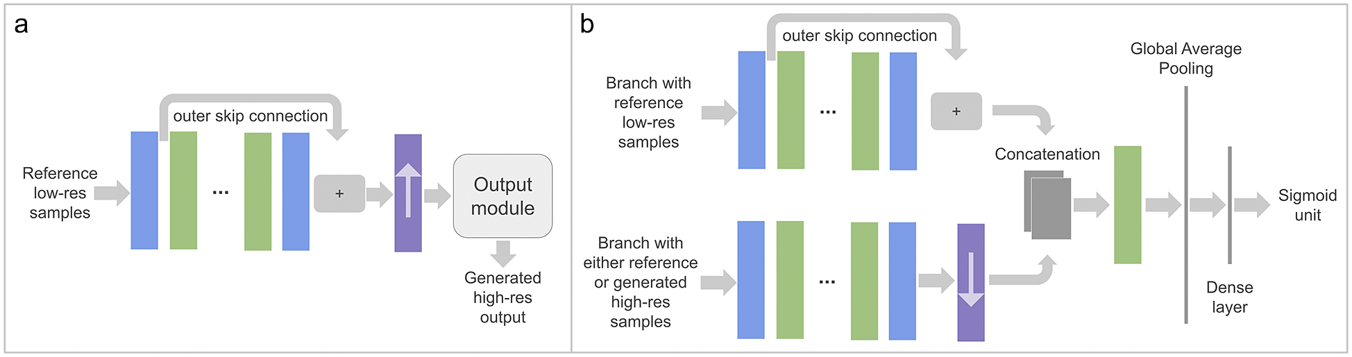
Figure 4. Example of a conditional generative adversarial model for spatiotemporal samples in post-upsampling mode (see Section 3.4.1). Two networks, the generator shown in panel (a), and discriminator shown in panel (b), are trained together optimizing an adversarial loss (see Section 3.5). The color legend for the blocks used here is shown in Figure 2a.
When working with DL4DS, the training strategy is controlled by choosing one of the training classes: dl4ds.SupervisedTrainer or dl4ds.CGANTrainer, for using supervised or adversarial losses accordingly.
4. Experimental Results
Downscaling applications are highly dependent on the target variable/dataset at hand, and therefore the optimal model architecture should be found in a case-by-case basis. In this section, we give a taste of the capabilities of DL4DS without conducting a rigorous comparison of model architectures and learning configurations. For our tests, we use data from the Copernicus Atmosphere Monitoring Service (CAMS) reanalysis (Inness et al., Reference Inness, Ades, Agust-Panareda, Barré, Benedictow, Blechschmidt, Dominguez, Engelen, Eskes, Flemming, Huijnen, Jones, Kipling, Massart, Parrington, Peuch, Razinger, Remy, Schulz and Suttie2019), the latest global reanalysis dataset of atmospheric composition produced by the European Centre for Medium-Range Weather Forecasts (ECMWF), which provides estimates of Nitrogen dioxide (NO2) surface concentration. We select NO2 data from the period between 2014 and 2018 at a 3-hourly temporal resolution which results in
 $ \sim $
14.6 k temporal samples. For our low-resolution dataset, we use the CAMS global reanalysis (CAMSRA) with a horizontal resolution of
$ \sim $
14.6 k temporal samples. For our low-resolution dataset, we use the CAMS global reanalysis (CAMSRA) with a horizontal resolution of
 $ \sim $
80 km. Our high-resolution target is the CAMS regional reanalysis produced for the European domain with a spatial resolution of
$ \sim $
80 km. Our high-resolution target is the CAMS regional reanalysis produced for the European domain with a spatial resolution of
 $ \sim $
10 km (0.1°). We also include predictor atmospheric variables from the ECMWF ERA5 reanalysis (Hersbach et al., Reference Hersbach, Bell, Berrisford, Hirahara, Horányi, Muñoz-Sabater, Nicolas, Peubey, Radu, Schepers, Simmons, Soci, Abdalla, Abellan, Balsamo, Bechtold, Biavati, Bidlot, Bonavita, De Chiara, Dahlgren, Dee, Diamantakis, Dragani, Flemming, Forbes, Fuentes, Geer, Haimberger, Healy, Hogan, Hólm, Janisková, Keeley, Laloyaux, Lopez, Lupu, Radnoti, de Rosnay, Rozum, Vamborg, Villaume and Thépaut2020), namely 2 m temperature and 10 m wind speed, with an intermediate resolution of
$ \sim $
10 km (0.1°). We also include predictor atmospheric variables from the ECMWF ERA5 reanalysis (Hersbach et al., Reference Hersbach, Bell, Berrisford, Hirahara, Horányi, Muñoz-Sabater, Nicolas, Peubey, Radu, Schepers, Simmons, Soci, Abdalla, Abellan, Balsamo, Bechtold, Biavati, Bidlot, Bonavita, De Chiara, Dahlgren, Dee, Diamantakis, Dragani, Flemming, Forbes, Fuentes, Geer, Haimberger, Healy, Hogan, Hólm, Janisková, Keeley, Laloyaux, Lopez, Lupu, Radnoti, de Rosnay, Rozum, Vamborg, Villaume and Thépaut2020), namely 2 m temperature and 10 m wind speed, with an intermediate resolution of
 $ \sim $
25 km (0.25°). Finally, we include as static variables: topography from the Global Land One-km Base Elevation Project and a land-ocean mask derived from it, and a layer with the urban area fraction derived from the land cover dataset produced by the European Space Agency. In order to make our test less heavy on memory requirements, we spatially subset the data and focus on the western Mediterranean region, as shown in Figure 5.
$ \sim $
25 km (0.25°). Finally, we include as static variables: topography from the Global Land One-km Base Elevation Project and a land-ocean mask derived from it, and a layer with the urban area fraction derived from the land cover dataset produced by the European Space Agency. In order to make our test less heavy on memory requirements, we spatially subset the data and focus on the western Mediterranean region, as shown in Figure 5.
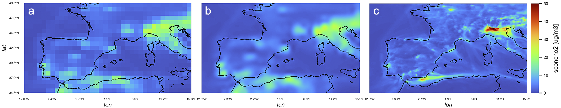
Figure 5. A reference NO2 surface concentration field from the low-resolution CAMS global reanalysis is shown in panel (a). In panel (b), we present a resampled version, via bicubic interpolation, of the low-resolution reference field. This interpolated field looks overly smoothed and showcases the inefficiency of simple resampling methods at restoring fine-scale information. Panel (c): the corresponding high-resolution field from the CAMS regional reanalysis. Both low- and high-resolution grids were taken from the holdout set for the same time step. The maximum value shown corresponds to the maximum value in the high-resolution grid.
We showcase eight models trained with DL4DS, without the intention of a full exploration of possible architectures and learning strategies. Different loss functions, backbones, learning strategies, and other parameters are combined in the model architectures detailed in Table 1. The training is carried out using a single cluster node with four NVIDIA V100 GPUs. The data is split into train and test sets by reserving the last year of data for test and validation. We fit the dl4ds.StandardScaler on the training set (getting the global mean and standard deviation) and applied it to both training and test sets (subtracting the global mean and dividing by the global standard deviation). All models are trained with the Adam optimizer (Kingma and Ba, Reference Kingma, Ba, Bengio and LeCun2015), for 100 epochs in the case of supervised CNNs and 18 epochs in the case of the conditional adversarial models.
Table 1. DL4DS models showcased in Section 4.

Figure 6 shows examples of predicted high-resolution fields produced by the models detailed in Table 1 and corresponding to the reference fields of Figure 5. These give a visual impression of the reconstruction ability of each model. Figures 7 and 8 show the Pearson correlation and Root Mean Square Error (RMSE) for each one of the aforementioned models. The metrics in these maps are computed for each grid point independently and for the whole year of 2018 (containing 2,920 holdout grids). Table 2 gives a more complete list of metrics (including the MAE, SSIM, and peak signal-to-noise ratio [PSNR]) computed for each grid pair separately (time step) and then summarized by taking the mean and standard deviation over the samples of the holdout year.


Figure 7. Pixel-wise Pearson correlation for each model, computed for the whole year of 2018.
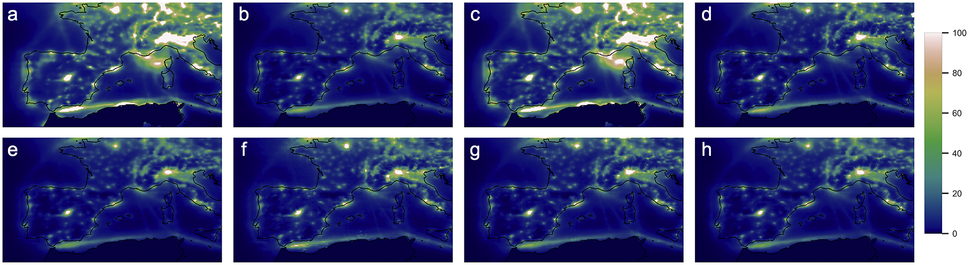
Figure 8. Pixel-wise RMSE for each model, computed for the whole year of 2018. The dynamic range is shared for all the panels, with a fixed maximum value to facilitate the visual comparison.
Table 2. Metrics computed for each time step, downscaled product with respect to the reference grid, of the holdout year for the models showcased in this section.
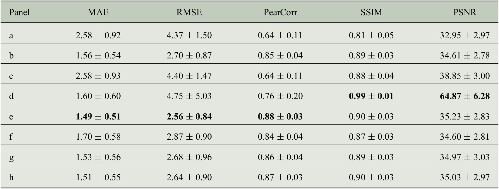
Note. Best models depending on the loss/metric used. Model d is the best for SSIM and PSNR (related) metrics. Model e for MAE-RMSE-PearCor.
Abbreviations: MAE, mean absolute error; PSNR, peak signal-to-noise ratio; RMSE, root-mean-square error; SSIM, structural similarity index measure.
For this particular task and datasets, and according to the metrics of Table 2, we find that models trained in MOS fashion perform better than those in PerfectProg and that a supervised model with residual blocks and subpixel convolution upsampling provides the best results. Also, we note that models trained with an LCB perform better than those without it, thanks to the fact that the LCB learns grid point- or location-specific weights. As expected, when the same network is optimized with respect to a DSSIM+MAE loss, it reaches higher scores in the SSIM and PSNR metrics. Training the CGAN model for more epochs could improve the results but would require longer runtimes and computational resources.
5. Summary and Future Directions
In this paper, we have presented DL4DS, a Python library implementing state-of-the-art and novel DL algorithms for empirical downscaling of gridded data. It is built on top of Tensorflow/Keras (Chollet et al., Reference Chollet2015), a modern and versatile DL framework. Among the key strengths of DL4DS are its simple API consisting of a few user-facing classes controlling the training procedure, its support for distributed GPU training (via data parallelism) powered by Horovod (Sergeev and Balso, Reference Sergeev and Balso2018), the generous number of customizable DL-based architectures included, the possibility of composing new architectures based on the general purpose building blocks offered, the option of saving and retraining models, and its support of different downscaling frameworks that learn either with explicit low-resolution and high-resolution data (MOS-like) or only with a high-resolution dataset (PerfectProg-like). DL4DS is a powerful tool for reproducible empirical downscaling experiments and for network architecture optimization. A thorough ablation study varying the depth and width of each backbone, in combination with other design choices, such as the upsampling method, and tested over several benchmark datasets, shall allow a complete comparison of CNN-based DL models for empirical downscaling.
DL has shown promise in post-processing and bias correction tasks (Rasp and Lerch, Reference Rasp and Lerch2018; Grönquist et al., Reference Grönquist, Yao, Ben-Nun, Dryden, Dueben, Li and Hoefler2020), so a natural research direction is to explore the application of DL4DS to related post-processing problems. Other interesting research directions are the implementation of uncertainty estimation techniques besides Monte Carlo dropout, the extension of DL4DS models to the case of non-gridded reference data (observational station data), the implementation of alternative adversarial losses such as the Earth mover’s distance (Wasserstein GAN), and the inclusion of alternative DL algorithms such as normalizing flows (Groenke et al., Reference Groenke, Madaus and Monteleoni2020).
Acknowledgments
We wish to acknowledge F. J. Doblas-Reyes, K. Serradell, H. Petetin, Ll. Lledó, and Ll. Palma for helpful discussions and comments, and P-A. Bretonnière and M. Samsó for assistance with data management.
Author Contributions
Formal analysis: C.A.G.G; Investigation: C.A.G.G; Methodology: C.A.G.G; Software: C.A.G.G; Visualization: C.A.G.G; Writing—original draft: C.A.G.G; Writing—review and editing: C.A.G.G.
Competing Interests
The author declares no competing interests exist.
Data Availability Statement
DL4DS code repository: https://github.com/carlos-gg/dl4ds.
Funding Statement
C.A.G.G. acknowledges funding from the European Union’s Horizon 2020 research and innovation program under the Marie SkÅ‚ odowska-Curie grant agreement H2020-MSCA-COFUND-2016-754,433.
Provenance
This article is part of the Climate Informatics 2022 proceedings and was accepted in Environmental Data Science on the basis of the Climate Informatics peer review process.


 Open access