


Impact Statement
This article contributed to the understanding of monthly rainfall forecasting in the Benin Republic. This was done through the development of a new monthly forecasting model using an artificial neural network approach. A large contribution of this work is the quantitative prediction of monthly rainfall 2 months in advance. This kind of forecasting allows policymakers and local populations to better plan their activities and to act appropriately ahead of time in order to mitigate the challenges of managing rainwater supplies, drought, and flooding.
1. Introduction
Rainfall is one of the weather parameters that mostly affect human life and livelihood around the world. In the current context of climate change and variability, accurate rainfall prediction is essential for mitigating floods, managing water resources, and safeguarding lives, property, and economic endeavors. Moreover, the capacity to predict rainfall several months ahead could improve water efficiency.
Forecasting the weather is a process of using the science and technology to make predictions about the state of the atmosphere at a specific location in the future. Soft computational methods and machine learning (ML) approaches have seen wide use in weather forecasting. ML algorithms are a promising alternative to numerical weather prediction methods because they can handle the complexity and volume of weather data with less computing power. ML, particularly neural networks, can detect complex patterns and nonlinear relationships in data. They have been used in predicting rainfall, predicting temperature, and modeling rainfall runoff. Artificial neural network (ANN) models are the most popular and widely used models for rainfall prediction because physical processes affecting rainfall occurrence are highly complex and nonlinear (Adamowski and Sun, Reference Adamowski and Sun2010). Recently, there has been a growing popularity in deep learning (DL) techniques due to recent technological advancements. Modeling sequential data using recurrent neural networks (RNNs) is a highly active field of research in DL (Xu et al., Reference Xu, Hu, Wu, Jian, Li, Chen, Zhang, Zhang and Wang2022). The long short-term memory (LSTM) technique is an innovative advancement in this domain that specifically targets the acquisition of long-term dependencies. It was created to tackle the issue of the vanishing gradient problem encountered in traditional RNNs (Hu et al., Reference Hu, Wu, Li, Jian, Li and Lou2018).
Many studies using ANNs to predict rainfall have been published. Ayodele and Precious (Reference Ayodele and Precious2019) used ANNs and the back propagation (BP) algorithm to forecast seasonal rainfall in Ikeja, Nigeria, using as input variables sea surface temperature (SST), U-wind at (surface, 700, 850, and 1000 hPa), air temperature, specific humidity, ITD, and relative humidity from year 1986 to 2017. Results of the proposed ANN show an accurate seasonal rainfall forecast for Ikeja with a limited error. Besides, Bello et al. (Reference Bello, Mamman, Zhang, Luo, Duan, Vishnoi, Kumar and Murugan2018) made an attempt at predicting rainfall over Kano in Nigeria using ANN and a linear model for a 3-month lead period. Comparing the results, ANN gave better accuracy. Abdulkadir et al. (Reference Abdulkadir, Salami, Aremu, Ayanshola and Oyejobi2017) used a similar approach to assess the efficacy of neural networks in predicting rainfall patterns in seven chosen stations in Nigeria using successive rainfall depth data as input. After the model validation, significant correlation coefficients were observed, indicating that ANN may be employed for quantitative rainfall prediction in these locations. Similarly, Ewona et al. (Reference Ewona, Osang, Uquetan, Inah and Udo2016) used ANNs to forecast rainfall across 23 sites in Nigeria using 30-year data. The predictability of rainfall was shown to be more accurate at higher latitudes across the country. Moreover, Folorrunsho (Reference Folorrunsho2014) also developed an ANN-based model for monthly rainfall forecasting in Zaria, Nigeria, using temperature, relative humidity, wind speed, and sunshine hours as input variables. The authors obtained a value of 81% as correlation coefficient (r) during the testing phase. Furthermore, Kashiwao et al. (Reference Kashiwao, Nakayama, Ando, Ikeda, Lee and Bahadori2017) compared multilayer perceptron (MLP) with a hybrid algorithm composed of BP and random optimization methods and radial basis function network (RBFN) for the purpose of forecasting short-term rainfall using data from the Japan Meteorological Agency. The authors demonstrated that MLP outperformed RBFN. Choubin et al. (Reference Choubin, Khalighi-Sigaroodi, Malekian and Kiis2016) compared multiple linear regression, MLP, and adaptive neuro-fuzzy inference system models for predicting precipitation in Iran. The metric results showed that the MLP network outperformed the other models in terms of performance. ANNs have been successfully used in conjunction with BP algorithm to forecast rainfall in Indonesia (Hardwinarto et al., Reference Hardwinarto and Aipassa2015). In Queensland, Australia, Abbot and Marohasy (Reference Abbot and Marohasy2014) used ANN and Predictive Ocean Atmosphere Model for Australia (POAMA) to forecast rainfall. Rainfall, minimum and maximum temperatures, the Inter-decadal Pacific Oscillation, the Dipole Mode Index, the Southern Oscillation Index, and El Nino 3.4 were used as input variables. In comparison to the POAMA model, the analysis discovered that the ANN model makes predictions that are more accurate. Three distinct models for monthly rainfall forecasting were developed by MuttalebAlhashimi (Reference MuttalebAlhashimi2014). From 1970 to 2008, the study collected monthly data on precipitation, mean temperature, wind speed, and relative humidity. The findings demonstrated the superiority of ANN models over other models. Pai et al. (Reference Pai, Pramod and Balchand2014) forecasted Southwest Indian Monsoon rainfall with ANN using SST, sea level pressure, humidity, and zonal (u) and meridional (v) winds. The findings demonstrate a fair degree of precision. In addition, Chen et al. (Reference Chen, Zhang, Kashani, Jun, Bateni, Band, Dash and Chau2022) evaluated the predictive accuracy of LSTM and random forest (RF) models for monthly rainfall prediction at two meteorological stations in Turkey, using rainfall as the input variable. The results demonstrated that the LSTM model exhibited superior performance compared to the RF model in terms of efficacy. Ni et al. (Reference Ni, Wang, Singh, Wu, Wang, Tao and Zhang2020) also created two hybrid models for predicting monthly streamflow and rainfall, using the conventional LSTM model as a basis. The findings showcased the aptness of LSTM for forecasting time series data. Kumar et al. (Reference Kumar, Singh, Samui and Jha2019) employed innovative DL models, specifically RNN and LSTM, to predict monthly rainfall in regions of India with consistent rainfall patterns. The findings demonstrate the successful application of DL networks in hydrological time series analysis. Additional applications using ML algorithms in the field of meteorology can be found in Demir and Citakoglu (Reference Demir and Citakoglu2023), Citakoglu (Reference Citakoglu2021), Lakshminarayana et al. (Reference Lakshminarayana, Singh, Mittal, Kothari, Yadav and Sharma2020), Fahimi et al. (Reference Fahimi, Yaseen and El-shafie2017), Yaseen et al. (Reference Yaseen, El-Shafie, Jaafar, Afan and Sayl2015), and Nourani et al. (Reference Nourani, Baghanam, Adamowski and Kisi2014).
Monthly rainfall plays a significant role in agricultural and hydrological endeavors (Omotosho et al., Reference Omotosho, Balogun and Ogunjobi2000). In the Republic of Benin, the majority of the population relies on agriculture that is dependent on rainfall. The study conducted by Amegnaglo et al. (Reference Amegnaglo, Anaman, Mensah-Bonsu, Onumah and Gero2017) examined the significance of seasonal climate forecasts for maize farmers in the Republic of Benin. The findings revealed that farmers highly value rainfall forecasts, particularly those that are accessible 1–2 months prior to the start of the rainy season. This variable provides information on water stress, deficits, and extreme climatic occurrences during the rainy season. Predicting rainfall accurately is a major challenge in operational water resource management in many countries, including the Republic of Benin.
Although much work has been done on rainfall prediction using ANNs, particularly MLP and LSTM approaches in different countries, so far, no study has established a rainfall-forecasting model for Benin Republic using those approaches. Our research focuses on accurately predicting monthly rainfall 2 months ahead in order to provide sufficient time for decision-making based on the predictions using ANNs. This study is unique in that it builds a new method for predicting models based on MLP network. To the best of our knowledge, this is the first time an MLP has been used to predict monthly rainfall for localized regions in the Benin Republic. Furthermore, this article examines and compares the performance of MLP against other techniques, such as LSTM and CF. The findings of this research will serve as a baseline for future researchers.
2. Materials and methods
2.1. Site description
Geographically located in West Africa at a latitude of 6°30′N to 12°30′N and a longitude of 1°E to 3°40′E, the Republic of Benin has 12 departments, of which six host main synoptic weather stations operated by the National Meteorological Agency of Benin, Agence Nationale de la Météorologie du Bénin (METEO-BENIN). Therefore, this study was focused on those six departments. Figure 1 shows the spatial location of selected synoptic weather stations in the study area. The geographical positions of selected stations are presented in Table 1. The purpose of selecting these places was to study the performance of the prediction models under diverse climatic and hydrological regimes. Benin’s climatic profile shows two contrasting climatic zones (Guinean vs. Sudanian) and a transitional zone (Sudano-Guinean). Figure 2 shows the rainfall patterns in different climate zones using rainfall data over a period from 1959 to 2021. The Guinean zone, located between 6°25′ and 7°30′N, has a subequatorial climate with four seasons (two rainy and two dry). The annual rainfall of approximately 1200 mm is bimodal, occurring mostly between March and July and September and November. The temperature ranges between 25 °C and 29 °C, and the relative humidity ranges between 69% and 97%. The Sudano-Guinean, located between 7°30′ and 9°45′N, is a transitional zone with two rainy seasons merging into a unimodal regime. Annual rainfall varies between 900 and 1110 mm, the temperature ranges between 25 °C and 29 °C, and the relative humidity ranges from 31% to 98%. The Sudanian region, which lies between 9°45′ and 12°25′N, has a tropical dry climate of two seasons of similar duration (rainy and dry). Annual mean rainfall in this region is often less than 1000 mm and occurs mostly between May and September. The temperature varies between 24 °C and 31 °C, and the relative humidity varies between 18% and 99% (Hounkpèvi et al., Reference Hounkpèvi, Tosso, Gbèmavo, Kouassi, Koné and Glèlè Kaka2016).

Figure 1. Study sites location: (a) Benin’s location in West Africa. (b) Synoptic stations’ location in Benin.
Table 1. Summary of the latitude and longitude coordinates for the chosen stations


Figure 2. Rainfall patterns in different climate zones in Benin Republic (period 1959–2021).
2.2. Data
Two climate datasets were used for this study:
-
• Monthly in situ rainfall (RR) data used as predictand was collected from the six weather stations for 63 years within the period from 1959 to 2021. The rainfall time series has been taken from METEO-BENIN.
-
• Monthly reanalysis atmospheric data for each station, collected as predictors of RR, comprises several key variables, including 10-meter wind speed, 2-meter temperature, evaporation, mean sea level pressure, surface pressure, relative humidity at 850 and 1000 millibars levels, zonal and meridional wind components at both 850 and 1000 millibars levels, and SST. These variables are monthly ERA5 data sourced from the Climate Data Store (CDS) (https://cds.climate.copernicus.eu), available for 1940–present (Hersbach et al., Reference Hersbach, Bell, Berrisford, Biavati, Horányi, Muñoz Sabater, Nicolas, Peubey, Radu and Rozum2023a,Reference Hersbach, Bell, Berrisford, Biavati, Horányi, Muñoz Sabater, Nicolas, Peubey, Radu and Rozumb). In this study, we considered the timeframe from January 1959 to December 2021. Table 2 presents the description of atmospheric data.
Table 2. Description of atmospheric data

2.3. Artificial neural networks
ANN is a soft computing method that mimics the behavior of biological neural processing (Graupe, Reference Graupe2013). ANN is a nonlinear statistical technique that has become popular among scientists as an alternative technique for predicting and modeling complicated time series, weather phenomena, and climate variables (Mekanik and Imteaz, Reference Mekanik and Imteaz2013). Various neural network architectures exist, but the prevalent design is the MLP neural network, developed in 1960 and, over time, becoming one of the most widely adopted methods for addressing a wide range of problems (Ren et al., Reference Ren, Li, Ren, Song, Xu, Deng and Wang2021). The MLP is characterized by an arrangement comprising an input layer, one or more hidden layers, and an output layer, which is trained using the backpropagation learning algorithm (Dawson and Wilby, Reference Dawson and Wilby1998). The input layer initially receives the data, the hidden layer processes them, and finally, the output layer displays the model’s output. Figure 3 presents an MLP with two hidden layers. The mathematical equation of an MLP with one hidden layer can be expressed as follows (Eq. 1).

Figure 3. A multilayer perceptron with two hidden layers. Source: Salaeh et al. (Reference Salaeh, Ditthakit, Pinthong, Hasan, Islam, Mohammadi and Linh2022).
 $$ {\hat{y}}_k={f}_2\left[\sum \limits_{h=1}^n{w}_{h\mathrm{o}}{f}_1\left(\sum \limits_{i=1}^m{w}_{i\mathrm{h}}{x}_i+{w}_{\mathrm{bh}}\right)+{w}_{\mathrm{bo}}\right] $$
where
 $ {\hat{y}}_k $
is the forecasted kth output value,
$ {\hat{y}}_k $
is the forecasted kth output value,
 $ {f}_2 $
is the activation function for the output neuron,
$ {f}_2 $
is the activation function for the output neuron,
 $ n $
is the number of hidden neurons,
$ n $
is the number of hidden neurons,
 $ {w}_{\mathrm{ho}} $
is the weight connecting the hth neuron in the hidden layer and neuron in the output layer,
$ {w}_{\mathrm{ho}} $
is the weight connecting the hth neuron in the hidden layer and neuron in the output layer,
 $ {f}_1 $
is the activation function for the hidden neuron,
$ {f}_1 $
is the activation function for the hidden neuron,
 $ m $
is the number of input neurons,
$ m $
is the number of input neurons,
 $ {w}_{i\mathrm{h}} $
is the weight connecting the ith neuron in the input layer and hth neuron in the hidden layer,
$ {w}_{i\mathrm{h}} $
is the weight connecting the ith neuron in the input layer and hth neuron in the hidden layer,
 $ {x}_i $
the ith input variable,
$ {x}_i $
the ith input variable,
 $ {w}_{\mathrm{b}h} $
is the bias for the hth hidden neuron, and
$ {w}_{\mathrm{b}h} $
is the bias for the hth hidden neuron, and
 $ {w}_{\mathrm{bo}} $
is the bias for output neuron.
$ {w}_{\mathrm{bo}} $
is the bias for output neuron.
In addition to their capacity to implicitly identify complex nonlinear relationships between variables, ANNs offer the advantage of requiring less formal statistical training for model development. ANNs are capable of revealing a wide range of interactions between predictor variables and can be trained using a variety of techniques. The primary disadvantages of ANN, however, are their “black box” nature and inability to discern causal relationships with clarity. Determining the optimal model structure prior to conducting studies is one of the methodological concerns that arise with the empirical construction of ANN models (Uncuoglu et al., Reference Uncuoglu, Citakoglu, Latifoglu, Bayram, Laman, Ilkentapar and Oner2022).
Since Hochreiter and Schmidhuber (Reference Hochreiter and Schmidhuber1997) proposed the LSTM neural network, it is widely used to accurately model short and long-term data. LSTMs are specifically designed to effectively capture and retain long-term dependencies. The differentiation between LSTM and conventional RNNs lies in their respective internal architectures. One of the most salient features of the LSTM model is its cell state, which facilitates the propagation of information across the entire sequence through a series of linear interactions (Pérez-Alarcón et al., Reference Pérez-Alarcón, Garcia-Cortes, Fernández-Alvarez and Martnez-González2022).
The LSTM architecture has an input gate, output gate, forget gate, and cell. The cell retains information for varying times. The forget gate is crucial in deciding what memory block information to discard. In contrast, the input gate receives new data and decides whether to update each node’s values, which the output gate then displays or discards. The structure of the LSTM unit is depicted in Figure 4, and the corresponding formula is presented in Eq. (2). To predict, a dense neural network layer connects the cell and hidden states to output (
 $ {y}_{out} $
, Eq. 3) after the input sequence (Mbuvha et al., Reference Mbuvha, Adounkpe, Houngnibo, Mongwe, Nikraftar, Marwala and Newlands2023).
$ {y}_{out} $
, Eq. 3) after the input sequence (Mbuvha et al., Reference Mbuvha, Adounkpe, Houngnibo, Mongwe, Nikraftar, Marwala and Newlands2023).
 $$ \left\{{c}_t,{h}_t\right\}={f}_{\mathrm{LSTM}}\left({x}_t,{c}_{t-1},{h}_{t-1},W\right) $$
 $$ {y}_{out}=\Phi \left({c}_t,{h}_t,{W}_d\right) $$
where
 $ W $
represents the weight matrices of the model,
$ W $
represents the weight matrices of the model,
 $ {x}_t $
is the input data,
$ {x}_t $
is the input data,
 $ {C}_{t-1} $
is the previous cell state,
$ {C}_{t-1} $
is the previous cell state,
 $ {h}_{t-1} $
is the previous hidden state,
$ {h}_{t-1} $
is the previous hidden state,
 $ {C}_t $
is the new cell state,
$ {C}_t $
is the new cell state,
 $ {h}_t $
is the new hidden state,
$ {h}_t $
is the new hidden state,
 $ \Phi $
and
$ \Phi $
and
 $ {W}_d $
represent the dense layer and its weight, respectively.
$ {W}_d $
represent the dense layer and its weight, respectively.

Figure 4. Structure of LSTM unit. Source: Nifa et al. (Reference Nifa, Boudhar, Ouatiki, Elyoussfi, Bargam and Chehbouni2023).
Long training times and memory demands are LSTM’s main drawbacks. Due of their sensitivity to random weight initializations, LSTM dropout implementation is difficult (Uncuoglu et al., Reference Uncuoglu, Citakoglu, Latifoglu, Bayram, Laman, Ilkentapar and Oner2022).
2.4. Climatology forecast
A climatology forecast (CF) is a prediction that relies exclusively on the mean or average value of the variable being studied, calculated using historical data over a specific time period. This historical average is then used as the forecast for future instances in the verification data. Thus, a climatology-based forecast suggests that the variable’s value at the forecast’s valid time will be equal to this average (Murphy, Reference Murphy1992). For instance, if the climatological average of monthly rainfall for June is 350 mm, then the CF forecast for June of the upcoming year would also be 350 mm.
The climatological average is determined by calculating the mean of the variable of interest over all historical data. Mathematically, this can be expressed as follows (Eq. 4):
 $$ \overline{x}=\frac{1}{n}\sum \limits_{i=1}^n{x}_i $$
where
 $ \overline{x} $
is the climatological average, n denotes the total number of observations in the historical data, and
$ \overline{x} $
is the climatological average, n denotes the total number of observations in the historical data, and
 $ {x}_i $
represents each observation.
$ {x}_i $
represents each observation.
The CF method provides a simple, interpretable forecast, but it has limitations. The method assumes past climate patterns will persist into the future, which may not be true due to climate change or other factors. In our study, the CF method is used as a fundamental baseline for comparison, and the CF period is 1991–2020, as recommended by the WMO (2021).
2.5. Methodology
The methodology is illustrated in Figure 5 and comprises five main stages: data acquisition and transformation (i), predictor selection (ii), data preprocessing (iii), model development (iv), and prediction and assessment (v). This study selected two ML methods, namely MLP and LSTM, to compare and evaluate their effectiveness in predicting monthly rainfall at six weather stations located in the Benin Republic. The MLP and LSTM models were implemented using Python code. The open-source software package Keras (Chollet, Reference Chollet2015) installed on top of the Tensorflow framework was utilized. The programming interface used for this purpose was Jupyter Notebook, and Python modules such as TensorFlow, Keras, Sklearn, Numpy, Pandas, Matplotlib, and others were utilized. We conducted all experiments in this study using a device running the Windows 10 operating system, a core i7 CPU, and 12 GB of RAM.

Figure 5. Summary of the main methodology.
2.5.1. Data transformation
With the exception of two missing rainfall values for Parakou station, there are no missing values in the data obtained. These two values occurred in March and April 1991 and were filled, respectively, by the median and mean of the rainfall records in March and April for other years.
Atmospheric data are released over grid areas of 0.25° (~27 km) and are saved in Network Common Data Form files. Using the Python programming language, the data for each weather station were extracted into csv files by considering the local grid cell where the station is located (see Table 1 for coordinates). In order to identify basins, which are regions in the ocean that have an influence (well-correlated) on the rainfall patterns, and get their time series for respective stations, the correlation between station rainfall and the SST (-40N_50N,-40E_80E) has been computed (Figure 6). This basin is found by first determining the grid box that shows the highest correlation and then selecting the basin by considering the neighboring grid boxes centered on that grid box with the highest correlation. Following the selection of all the best-correlated basins, we computed the mean over each basin to obtain a monthly SST time series for each station.

Figure 6. Correlation map between station rainfall and grid point SST (-40N_50N,-40E_80E).
2.5.2. Selecting of optimal lagged predictors
Meteorological variables are potentially useful predictors of precipitation. To select the predictor variables and identify the months that could be used as input to the ANNs, cross-correlation analyses were carried out for delayed atmospheric data. The correlation coefficients were calculated between each monthly atmospheric data with a lag time from 1 to 6 months and monthly rainfall (Figure 7). To avoid data leakage, the test data (2018–2021) was not included when calculating the correlation coefficients. The lagged atmospheric variables with significant correlations at lags ranging from 3 to 6 months were selected as rainfall predictors. The presence of robust correlations beyond a lag of 2 months suggests that these variables have the potential to serve as rainfall predictors. This extended lag period offers an opportunity to establish early warning systems for various socio-economic sectors and facilitate informed decision-making processes (Gado Djibo et al., Reference Gado Djibo, Karambiri, Seidou, Sittichok, Philippon, Paturel and Moussa Saley2015). The list of predictors variables, values of the correlation coefficients and times lags (in red color) that were used for the forecasting model are shown in Table 3. For different atmospheric variables, different months had a significant correlation with rainfall.

Figure 7. Correlations between rainfall and atmospheric variables.
Table 3. Selected meteorological variable, lagged months (in red color), and correlation coefficients of monthly rainfall

2.5.3. Data preprocessing
The objective of the data preprocessing phase was to ensure correct data type and format conversion for all parameters, as well as normalize the data in order to maintain feature values within a specified range.
The final data set of 750 rows (July 1959–December 2021), representing the number of months of observation, is the data obtained after including lagged values as possible predictors, even if the data was collected from January 1950. In other words, July 1959 is the first instance with completed lagged values. First, we divided the data into three sets: the training, validation, and testing sets. The training set is used to update the network weights and biases; the validation set is used to guarantee the generalization capability of the model; and the test set is used to check the generalization (Mahmood, Reference Mahmood2017). The first 702 rows (July 1959–December 2017) were used to train and validate MLP and LSTM models. Then, 80% (561 rows, July 1959–March 2006) were used for training, while 20% (141 rows, April 2006–December 2017) were used for model validation and overfitting prevention. Model testing used the remaining 4 years of unseen data (48 rows, January 2018–December 2021).
Training a neural network with unscaled data with a wide range of values can slow learning and convergence. It may even prevent the network from learning the underlying problem. In order to address this concern, it is highly recommended to implement the practice of data normalization. This process entails adjusting the scale of the data to fall within the range of 0 and 1, thereby optimizing the learning process. Hence, the MinMaxScaler function was employed to normalize the input and output data within the range of 0 to 1, as described by Eqs. (5) and (6), respectively.
 $$ {\displaystyle \begin{array}{l}{X}_{\mathrm{n}}=\frac{X-{X}_{\mathrm{min}}}{X_{\mathrm{max}}-{X}_{\mathrm{min}}}\end{array}} $$
 $$ {\displaystyle \begin{array}{l}{Y}_{\mathrm{n}}=\frac{\ln \left(1+Y\right)-\min \left(\ln \left(1+Y\right)\right)}{\max \left(\ln \left(1+Y\right)\right)-\min \left(\ln \left(1+Y\right)\right)}\end{array}} $$
where
 $ X $
,
$ X $
,
 $ {X}_{\mathrm{min}} $
, and
$ {X}_{\mathrm{min}} $
, and
 $ {X}_{\mathrm{max}} $
are the value to be scaled, the minimum and maximum values of all records, respectively, and
$ {X}_{\mathrm{max}} $
are the value to be scaled, the minimum and maximum values of all records, respectively, and
 $ {X}_n $
is the normalized input value.
$ {X}_n $
is the normalized input value.
 $ {Y}_n $
is the normalized monthly rainfall value, and
$ {Y}_n $
is the normalized monthly rainfall value, and
 $ Y $
is the monthly rainfall value to be scaled.
$ Y $
is the monthly rainfall value to be scaled.
 $ \ln $
denotes the natural logarithm. Log transformation is used for normalization to have a less skewed distribution of the rainfall parameter.
$ \ln $
denotes the natural logarithm. Log transformation is used for normalization to have a less skewed distribution of the rainfall parameter.
To finish, the LSTM model’s architecture is a 3D input (number of samples, time steps, features). The dataset was then reshaped to fit these needs (561, 1, 12); (141, 1, 12); and (48, 1, 12) for training, validating, and testing, respectively.
2.5.4. Model development
An effective ANN model requires identifying key input variables and optimizing network structure. Input variables were selected by analyzing correlations between lagged atmospheric variables and monthly rainfall (see Figure 7). The number of hidden layers and neurons depends on the task and available data (Mekanik et al., Reference Mekanik, Imteaz, Gato-Trinidad and Elmahdi2013; Ghamariadyan and Imteaz, Reference Ghamariadyan and Imteaz2021). This study used one hidden layer in MLP and LSTM models. Given our limited sample size (750) and large predictor pool (12), this choice reduces overfitting. More hidden layers in an ANN increase complexity and reduce system performance. Thus, most scientists recommend a single hidden layer (Arifin et al., Reference Arifin, Robbani, Annisa and Ma’Arof2019). Since there is no standard method for estimating the optimal number of hidden layer neurons, we used trial-and-error (Hossain et al., Reference Hossain, Rasel, Imteaz and Mekanik2020; Bai et al., Reference Bai, Liu and Xie2021; Ghamariadyan and Imteaz, Reference Ghamariadyan and Imteaz2021; Tareke and Awoke, Reference Tareke and Awoke2023; Nifa et al., Reference Nifa, Boudhar, Ouatiki, Elyoussfi, Bargam and Chehbouni2023). This was achieved by training the model with different numbers of hidden neurons, from 10 to 20, and making a decision based on the root mean square error (MSE) and coefficient of determination of the predicted and observed values in the training and validation datasets, as well as by analyzing the loss function curve over the number of epochs. Because the ANN sets the initial weight value at random at the start of training, a different neural network model is created for each training process, resulting in different performance. As a result, the best prediction model was chosen by repeating the ANN model generation process 50 times for each hidden neuron selected. Additionally, we used an early stopping technique (Prechelt, Reference Prechelt1998) to prevent overfitting, stopping training when validation errors began increasing, even if training errors were decreasing. The number of epochs was set to 200 to have the same scale of comparison between models, with an early stop of 20 epochs when the model performance stops improving on the validation set. The optimizer used was the Adam optimizer, with a learning rate set at 0.001 and batch sizes of 8, 16, 32, and 64. The chosen loss function was the MSE (Eq. 7). In this study, the rectified linear unit, which keeps positive input values while setting negative input values to zero, and linear functions were considered for the hidden and output layers, respectively, in all of the models that were implemented.
 $$ {\displaystyle \begin{array}{l}\mathrm{MSE}=\frac{1}{n}\sum \limits_{i=1}^n{\left({y}_i-{\hat{y}}_i\right)}^2\end{array}} $$
where
 $ {y}_i $
and
$ {y}_i $
and
 $ {\hat{y}}_i $
are the observed and predicted values for the ith data point respectively, and
$ {\hat{y}}_i $
are the observed and predicted values for the ith data point respectively, and
 $ n $
is the number of samples.
$ n $
is the number of samples.
2.5.5. Model evaluation
The prediction performance of the models was assessed by comparing observed and predicted rainfall using five performance measures: the root mean squared error (RMSE), the mean absolute error (MAE) (Legates and McCabe Jr, Reference Legates and McCabe1999), the mean absolute percentage error (MAPE) (Uncuoglu et al., Reference Uncuoglu, Citakoglu, Latifoglu, Bayram, Laman, Ilkentapar and Oner2022), the coefficient of determination (R
2) (Etemadi et al., Reference Etemadi, Samadi and Sharifikia2014), and the Nash-Sutcliffe efficiency (NSE) coefficient (Nash and Sutcliffe, Reference Nash and Sutcliffe1970) (Eqs. 8–12). The RMSE and MAE metrics are commonly used in statistical modeling due to their theoretical importance. The RMSE is used to evaluate how closely the predicted values match the observed values, based on the relative range of the data. The MAE measures the average magnitude of the errors in a set of predictions, without considering their direction. The MAE and RMSE values range between 0 and
 $ \infty $
. The lower the RMSE and MAE, the better a model fits a dataset. It is well known that the MAE is less sensitive to outliers than the RMSE (Hyndman and Koehler, Reference Hyndman and Koehler2006). The MAPE has the advantage of being independent of the dependent variable’s order of magnitude. According to Uncuoglu et al. (Reference Uncuoglu, Citakoglu, Latifoglu, Bayram, Laman, Ilkentapar and Oner2022), if the MAPE criterion is less than 10%, the estimations are excellent, between 10% and 20%, good, between 20% and 50%, acceptable, and larger than 50%, inaccurate. R
2 evaluates the degree of correlation between predicted and observed data, under the assumption of a linear relationship (Choubin et al., Reference Choubin, Malekian, Samadi, Khalighi-Sigaroodi and Sajedi-Hosseini2017). It ranges from 0 to 1, with higher values indicating lower error variance. The NSE values range between -
$ \infty $
. The lower the RMSE and MAE, the better a model fits a dataset. It is well known that the MAE is less sensitive to outliers than the RMSE (Hyndman and Koehler, Reference Hyndman and Koehler2006). The MAPE has the advantage of being independent of the dependent variable’s order of magnitude. According to Uncuoglu et al. (Reference Uncuoglu, Citakoglu, Latifoglu, Bayram, Laman, Ilkentapar and Oner2022), if the MAPE criterion is less than 10%, the estimations are excellent, between 10% and 20%, good, between 20% and 50%, acceptable, and larger than 50%, inaccurate. R
2 evaluates the degree of correlation between predicted and observed data, under the assumption of a linear relationship (Choubin et al., Reference Choubin, Malekian, Samadi, Khalighi-Sigaroodi and Sajedi-Hosseini2017). It ranges from 0 to 1, with higher values indicating lower error variance. The NSE values range between -
 $ \infty $
and 1, with 1 being the perfect model. Negative NSE values indicate that the prediction model does not forecast better than the mean of the actual data.
$ \infty $
and 1, with 1 being the perfect model. Negative NSE values indicate that the prediction model does not forecast better than the mean of the actual data.
 $$ {\displaystyle \begin{array}{l}\mathrm{RMSE}=\sqrt{\frac{1}{n}\sum \limits_{i=1}^n{\left({\hat{y}}_i-{y}_i\right)}^2}\end{array}} $$
 $$ \mathrm{MAE}=\frac{1}{n}\sum \limits_{i=1}^n\left|{\hat{y}}_i-{y}_i\right| $$
 $$ {\displaystyle \begin{array}{l}\mathrm{MAPE}=100\frac{1}{n}\sum \limits_{i=1}^n\left|\frac{{\hat{y}}_i-{y}_i}{\overline{\hat{y}}}\right|\end{array}} $$
 $$ R2=\frac{{\left({\sum}_{i=1}^n\left({y}_i-\overline{y}\right).\left({\hat{y}}_i-\overline{\hat{y}}\right)\right)}^2}{\sum_{i=1}^n{\left({y}_i-\overline{y}\right)}^2.{\sum}_{i=1}^n{\left({\hat{y}}_i-\overline{\hat{y}}\right)}^2} $$
 $$ {\displaystyle \begin{array}{l}\mathrm{NSE}=1-\frac{\sum_{i=1}^n{\left({y}_i-{\hat{y}}_i\right)}^2}{\sum_{i=1}^n{\left({y}_i-\overline{y}\right)}^2}\end{array}} $$
From the above,
 $ {\hat{y}}_i $
and
$ {\hat{y}}_i $
and
 $ {y}_i $
are the model predictions and observed values, respectively; n is the number of target values;
$ {y}_i $
are the model predictions and observed values, respectively; n is the number of target values;
 $ \overline{\hat{y}} $
is the mean of predicted values; and
$ \overline{\hat{y}} $
is the mean of predicted values; and
 $ \overline{y} $
is the mean of observed values.
$ \overline{y} $
is the mean of observed values.
In addition to this, a Taylor diagram, violin plots, and box error were used to evaluate model accuracy. These diagrams show how well models match observations (Taylor, Reference Taylor2001; Choubin et al., Reference Choubin, Malekian, Samadi, Khalighi-Sigaroodi and Sajedi-Hosseini2017; Demir and Citakoglu, Reference Demir and Citakoglu2023; Coşkun and Citakoglu, Reference Coşkun and Citakoglu2023). The Taylor diagram illustrates the geometric relationship between correlation, centered root mean square difference, and standard deviation amplitude. On the other hand, a violin plot shows the dataset’s probability distribution using a boxplot and kernel density graphs on each side. Finally, the Kruskal–Wallis test was used to determine whether the prediction results have similar distribution as the actual data (Coşkun and Citakoglu, Reference Coşkun and Citakoglu2023).
3. Results and discussion
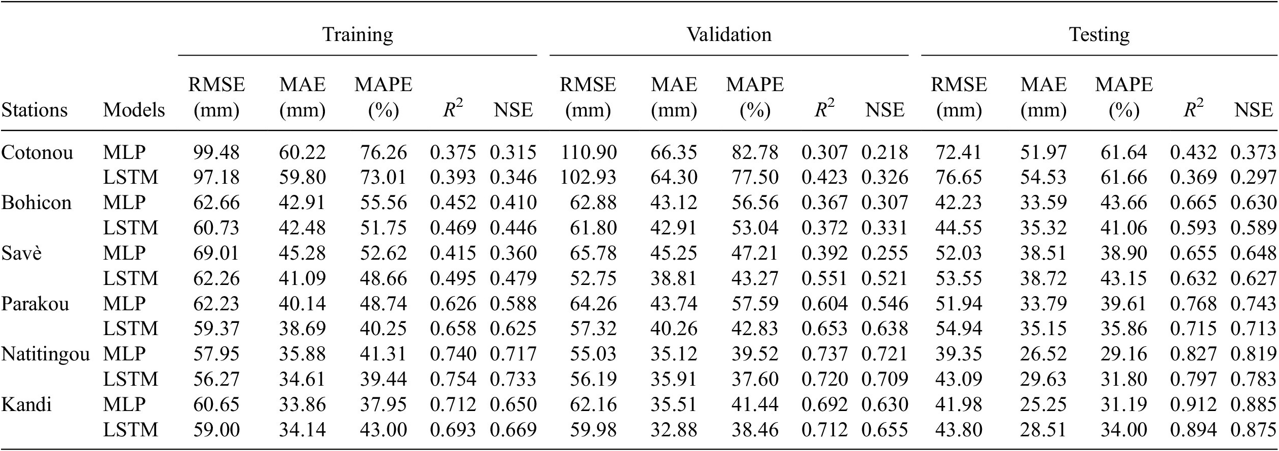
Table 4 presents the optimal values found for the number of hidden neurons and batch sizes for the models. The loss function during the training and validation phases of the selected network architecture is shown in Figure 8. As depicted in the figure, each model’s training and validation loss plots across all stations have been similar, with the same monotony. Hence, neither the models overfit nor underfit (Chollet, Reference Chollet2015). Table 5 shows the RMSE, MAE, MAPE, R 2, and NSE values obtained by the developed MLP and LSTM models over the training, validation, and testing datasets. During the test period, the metric for assessing performance RMSE values for MLP and LSTM models vary between 39.35 and 72.41 mm, and between 43.09 and 76.65 mm, respectively, depending on the weather station. Similarly, the MAE ranges from 25.25 to 51.97 mm for MLP and from 28.51 to 54.53 mm for LSTM. The MAPE values for MLP and LSTM models vary between 29.16% and 61.64%, and between 31.80% and 61.66%, respectively. The R 2 values range from 0.432 to 0.912 for MLP and from 0.369 to 0.894 for LSTM. Additionally, the NSE values vary between 0.373 and 0.885 for MLP and between 0.297 and 0.875 for LSTM, depending on the weather station. The MLP models exhibit superior accuracy compared to the LSTM models in monthly rainfall predictions across all locations, as evidenced by their lower RMSE, MAE and MAPE values, as well as higher R 2 and NSE values. The reason why LSTM did not perform better than MLP could be the limited size of the training dataset used. According to Cheng et al. (Reference Cheng, Fang, Kinouchi, Navon and Pain2020), the absence of a large monthly training dataset is what causes the LSTM model to perform less accurately on a monthly scale when compared to the ANN, but it performs better when it comes to making daily predictions.
Table 4. Optimal parameters used for training MLP and LSTM network

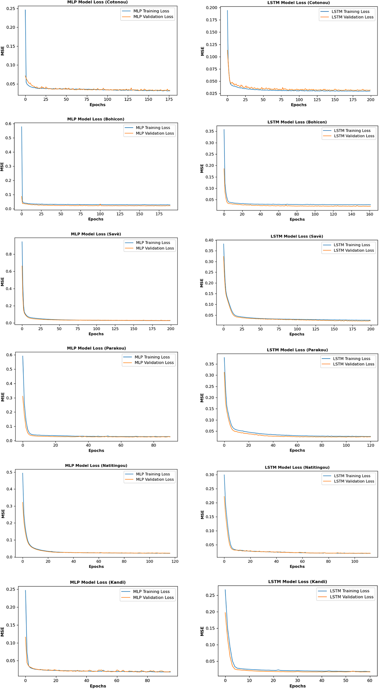
Figure 8. Loss function while training the MLP and LSTM models for all stations.
Table 5. RMSE, MAE, MAPE, R 2, and NSE values obtained over the training, validation, and testing datasets
In addition, we compared the results of the MLP model with those of the CF model to determine whether or not the MLP model actually performs significantly better than simply making the assumption that the climatologically typical amount of rainfall occurs each month. When it comes to medium- and long-term forecasting, CF is a better benchmark than persistence forecasts (Murphy,Reference Murphy1992). RMSE, MAE, R 2, and NSE for each model over the testing set are shown in Figure 9. During the test period, the CF achieved RMSE ranging from 40.43 to 74.54 mm, MAE from 27.90 to 54.30 mm, R 2 from 0.443 to 0.887, and NSE from 0.335 to 0.845, depending on the weather station. Similar to the MLP and LSTM, the best prediction with CF is also observed at Kandi, and the worst at Cotonou (see Figure 9). Based on NSE, the MLP model is the best compared to LSTM and CF in all stations except in Bohicon Station, where CF outperformed both MLP and LSTM. The NSE for the CF is 0.661 in this station, while the MLP and LSTM achieve 0.630 and 0.589, respectively. Also, aside from Bohicon, the LSTM model is unable to achieve higher accuracy than the CF for Cotonou in terms of NSE.

Figure 9. Prediction performance with the MLP, LSTM, and CF over the test period (2018–2021).
Hydrographs and scatterplots (Figures 10–15) were also used to compare observed and predicted monthly rainfall values during the test period (2018–2021).

Figure 10. Comparison between observed and predicted monthly rainfall using MLP, LSTM, and CF at Cotonou during the test period (2018–2021): (a) hydrograph and (b) scatterplot.
Figure 10 depicts the hydrographs of the MLP, LSTM, and CF model predictions versus observed monthly rainfall at Cotonou during the test period, as well as the scatterplots. The graphs show that the models do not have a high forecasting capability, with low NSE values (0.297, 0.335, and 0.373 for LSTM, CF, and MLP, respectively). Following the categorization of NSE values into four benchmark categories (Moriasi et al., Reference Moriasi, Arnold, Van Liew, Bingner, Harmel and Veith2007), all models’ performance could be classified as unsatisfactory (NSE ≤ 0.50). Furthermore, as shown in Figure 10(a), the actual and predicted time series are also not very close to each other, and high rainfall values are significantly underestimated at some peaks. The scatterplot in Figure 10(b) shows a good correlation for all low and medium data points.
Figure 11 shows the hydrographs of all of the models’ predictions in comparison to the observed monthly rainfall, as well as the scatterplots at Bohicon during the testing phase. The graphs demonstrate that the models have adequate forecasting capability, with relatively high NSE criteria (0.589, 0.630, and 0.661 for LSTM, MLP, and CF, respectively). According to Moriasi et al.’s (Reference Moriasi, Arnold, Van Liew, Bingner, Harmel and Veith2007) classification of NSE values into four benchmark categories, the performance of LSTM and MLP is deemed to be satisfactory (0.5 < NSE ≤ 0.65), whereas the performance of CF is deemed to be good (0.65 < NSE ≤ 0.75). The model predictions reasonably follow the series patterns. This can be seen in Figure 11(a). The scatterplot in Figure 11(b) shows that there is a good correlation for all data points across all ranges.

Figure 11. Comparison between observed and predicted monthly rainfall using MLP, LSTM, and CF at Bohicon during the test period (2018–2021): (a) hydrograph and (b) scatterplot.
Scatterplots and hydrographs of predicted versus observed monthly rainfall at Savè during the testing period are shown in Figure 12. NSE criterion values of 0.593 for CF, 0.627 for LSTM, and 0.648 for MLP are indicative of the models’ satisfactory forecasting ability. Based on the four benchmark categories of NSE values (Moriasi et al., Reference Moriasi, Arnold, Van Liew, Bingner, Harmel and Veith2007), all models demonstrate satisfactory performance (0.5 < NSE ≤ 0.65). Figure 12(a) shows that the actual and forecast time series are similar, with peak rainfall event captured by MLP model. The scatterplot in Figure 12(b) shows a good correlation for all data points in all ranges.

Figure 12. Comparison between observed and predicted monthly rainfall using MLP, LSTM, and CF at Savè during the test period (2018–2021): (a) hydrograph and (b) scatterplot.
The hydrographs of all model predictions versus observed monthly rainfall, as well as the scatterplots, at Parakou during the testing period, are displayed in Figure 13. The models’ good predictive ability is demonstrated by the graphs, which feature NSE criteria values of 0.704, 0.713, and 0.743 for CF, LSTM, and MLP, respectively. Following the breakdown of NSE values into four benchmark categories (Moriasi et al., Reference Moriasi, Arnold, Van Liew, Bingner, Harmel and Veith2007), all models exhibit good (0.65 < NSE ≤ 0.75) performance. The model predictions reasonably follow the series patterns, as seen in Figure 13(a), but high rainfall values are underestimated. In Figure 13(b), the scatterplot shows a good correlation between the displayed data points in all ranges.

Figure 13. Comparison between observed and predicted monthly rainfall using MLP, LSTM, and CF at Parakou during the test period (2018–2021): (a) hydrograph and (b) scatterplot.
Figure 14 depicts the hydrographs and scatterplots of all model predictions versus observed monthly rainfall at Natitingou during the testing period. The graphs show that the models can forecast well, with NSE criteria of 0.772, 0.783, and 0.819 for CF, LSTM, and MLP, respectively. All models exhibit very good (0.75 < NSE ≤ 1) performance, according to the classification of NSE values into four benchmark categories (Moriasi et al., Reference Moriasi, Arnold, Van Liew, Bingner, Harmel and Veith2007). As shown in Figure 14(a), the actual and forecast time series are nearly identical, with peak rainfall events almost captured. The scatterplot in Figure 14(b) shows a very good correlation for all data points in all ranges.

Figure 14. Comparison between observed and predicted monthly rainfall using MLP, LSTM, and CF at Natitingou during the test period (2018–2021): (a) hydrograph and (b) scatterplot.
Hydrographs and scatterplots of the monthly rainfall observed and predicted by each model during the testing period are displayed in Figure 15 for Kandi. The graphs present a very good capacity for forecasting on the part of the models, as evidenced by the high values of NSE criteria (0.845, 0.875, and 0.885 for CF, LSTM, and MLP, respectively). According to the classification of NSE values into four benchmark categories (Moriasi et al., Reference Moriasi, Arnold, Van Liew, Bingner, Harmel and Veith2007), all models exhibit very good (0.75 < NSE ≤ 1) performance. According to Figure 15(a), the actual and forecast time series are, for the most part, identical to one another, with peak rainfall events almost captured by MLP and LSTM models. The scatterplot that can be seen in Figure 15(b) demonstrates that there is a very good correlation between all of the data points across all of the ranges.

Figure 15. Comparison between observed and predicted monthly rainfall using MLP, LSTM, and CF at Kandi during the test period (2018–2021): (a) hydrograph and (b) scatterplot.
These results are confirmed in Figure 16, which depicts the evaluation metrics (correlation, RMSE, and standard deviation) for the MLP, LSTM, and CF models during the testing period as a Taylor diagram. This graphical summary of the agreement between model predictions and observations is quite helpful. It can be seen that the MLP model’s point (in red) is closer to the observed point (red star dot) than the LSTM and CF models in all stations, except in Bohicon, where the CF model is slightly closer than the MLP.

Figure 16. Taylor diagrams of MLP, LSTM, and CF for all stations.
Violin plot (Figure 17) and error boxplot (Figure 18) of the models were also used for comparison. According to Figure 17, the MLP model’s violin plots at all stations are more similar to the actual data sets than the LSTM and CF models. This suggests that MLP model estimated rainfall values are more statistically similar to actual data. Thus, the MLP model simulates rainfall better than the MLP and CF models at all stations. This is confirmed by the error boxplot diagram results. The observed values were subtracted from the predicted values to create the errors diagrams. Both violin and error boxplot results coincide with the Taylor diagram results, as can be seen from these results.

Figure 17. Violin plots of MLP, LSTM, and CF for all stations over the test period (2018–2021). Thin black lines represent the 5th and 95th percentile ranges of rainfall values, while thick black lines and white dots represent the 25th and 75th percentile ranges and median, respectively.

Figure 18. Errors boxplots of MLP, LSTM, and CF for all stations over the test period (2018–2021).
Finally, the Kruskal–Wallis test was employed to see if the predicted and observed data distributions matched. As seen in Table 6, all models’ rainfall data estimations reject the Ho hypothesis. The Kruskal–Wallis test results indicate that there was no significant difference between the means of the predicted and observed rainfall values. The predicted rainfall by MLP, LSTM, and CF is consistent with the observed rainfall, but the MLP model performs better. Although they could fairly accurately simulate monthly rainfall, the models were unable to replicate some of the highest monthly rainfall values. The size of the training data and the small number of heavy rainfall events may have made it difficult for models to learn such features (Pérez-Alarcón et al., Reference Pérez-Alarcón, Garcia-Cortes, Fernández-Alvarez and Martnez-González2022). Furthermore, the performance of all models’ predictions varies significantly, both within and between climate zones, with more accurate performance in the Sudanian climate zone having a unimodal rainfall regime and less accurate performance in the Guinean zone having a bimodal rainfall regime. This may be due to the increased instability and extreme rainfall in the Guinean zone of the study site. Additionally, the results demonstrate that variations in each region’s geographical characteristics have an impact on rainfall predictions, with better accuracy at higher latitudes. Ewona et al. (Reference Ewona, Osang, Uquetan, Inah and Udo2016) reported similar results by applying ANN to predict rainfall over 23 stations in Nigeria with more accurate rainfall predictability at higher latitudes over Nigeria. The correlation coefficients were in ascending order from south to north. When using ANN to predict rainfall at seven locations in Nigeria, Abdulkadir et al. (Reference Abdulkadir, Salami, Aremu, Ayanshola and Oyejobi2017) also reported similar results.
Table 6. P-values of Kruskal–Wallis test at 95% significance level

Ho: There are differences between mean predicted and observed values.
4. Conclusion and future work
Accurate rainfall prediction has always been a significant challenge since so many lives depend on it. Monthly rainfall forecasting has a number of advantages. Taking agriculture, water resource management, risk management, and disaster mitigation as examples, it helps decision-makers and stakeholders in these sectors. The aim of this study is to develop an ANN model to forecast monthly rainfall 2 months in advance for selected locations in the Benin Republic. This study also examined how geographical regions affected the model’s effectiveness in predicting monthly rainfall in Benin. To achieve this, an MLP approach has been proposed to predict monthly rainfall using 12 lagged atmospheric variables as predictors. When comparing the developed model to the LSTM and CF, the proposed MLP model was found to perform better, demonstrating the efficacy of MLP in a rainfall prediction task. We also found that rainfall predictability was more accurate at higher latitudes across the country.
According to the findings of this study, the MLP prediction model can be employed independently as a reliable model for rainfall predictions.
The study has six primary limitations: utilizing MLP and LSTM ML methods along with CF; employing six weather stations to depict Benin; utilizing reanalysis atmospheric data from 1959 to 2021 as predictors; employing cross-correlation analysis to select input features at different time lags; incorporating visual comparison criteria such as Taylor, violin, and error box plots alongside performance metrics; and utilizing the Kruskal–Wallis test to assess result accuracy.
Predicting rainfall is a complex process that requires continual improvement. Future work will be necessary to improve the performance of ANN models in predicting extreme rainfall events. This can be achieved by incorporating additional climate variables, employing ensemble techniques and specific training techniques, and further investigating the architecture of the network model in order to improve prediction accuracy.
In conclusion, this study demonstrated the feasibility of predicting monthly rainfall 2 months in advance for the study locations using ANNs and lagged atmospheric variables.
Acknowledgments
The authors are grateful to the National Meteorological Agency of Benin, Agence Nationale de la Météorologie du Bénin (METEO-BENIN), and ECMWF for providing in situ rainfall and reanalysis atmospheric data, respectively, for this work. The authors also thank the anonymous reviewers and editor for their valuable contributions to the manuscript.
Author contribution
Conceptualization: A.N.A. and K.O.O. Methodology: A.N.A., K.O.O., and F.K.O. Supervision: K.O.O. and F.K.O. Data curation: A.N.A. Data visualization: A.N.A. Writing original draft: A.N.A. and F.K.O. All authors approved the final submitted draft.
Competing interest
The authors declare that they have no conflict of interest.
Data availability statement
ERA5 reanalysis atmospheric data were retrieved online from the Climate Data Store (https://cds.climate.copernicus.eu), paying no fees. Data obtained from METEO-BENIN are available from Arsene A. with the permission of METEO-BENIN. Source codes, models, and data supporting the study’s findings will be made available through a GitHub repository upon reasonable request.
Ethics statement
The research meets all ethical guidelines, including adherence to the legal requirements of the study country.
Funding statement
The authors thank the West African Science Service Centre on Climate Change and Adapted Land Use (WASCAL) and the German Government, particularly the Federal Ministry of Education and Research (BMBF), for the financial support provided to Arsene A. through a Master’s scholarship and a research budget allocation.


 Open access