


Impact Statement
To achieve better climate predictions, we need to model aerosols with reduced computational effort. We accomplish this by using a neural network that accurately learns the input–output mapping from a traditional aerosol microphysics model, while being significantly faster. Physical constraints are added to make the emulator feasible for a stable long-term global climate model run.
1. Introduction
Aerosol forcing remains the largest source of uncertainty in the anthropogenic effect on the current climate (Bellouin et al., Reference Bellouin, Quaas, Gryspeerdt, Kinne, Stier, Watson-Parris, Boucher, Carslaw, Christensen, Daniau, Dufresne, Feingold, Fiedler, Forster, Gettelman, Haywood, Lohmann, Malavelle, Mauritsen, DT, Myhre, Mülmenstädt, Neubauer, Possner, Rugenstein, Sato, Schulz, Schwartz, Sourdeval, Storelvmo, Toll, Winker and Stevens2020). The aerosol cooling effect hides some of the positive radiative forcing caused by greenhouse gas emissions and future restrictions to lower air pollution might result in stronger observed warming. Aerosols impact climate change through aerosol–radiation interactions and aerosol–cloud interactions (IPCC, 2013). They can either scatter or absorb radiation, which depends on the particles’ compounds. Black carbon (BC) aerosols from fossil fuel burning, for example, have a warming effect by strongly absorbing radiation, whereas sulfate (SO4) from volcanic eruptions has a cooling effect by being less absorbing and primarily scattering radiation. Clouds influence the Earth’s radiation budget by reflecting sunlight and aerosols can change cloud properties significantly by acting as cloud condensation nuclei (CCN). A higher concentration of aerosols leads to more CCN which, for a fixed amount of water, results in more but smaller cloud droplets. Smaller droplets increase the clouds’ albedo (Twomey, Reference Twomey1974) and can enhance the clouds’ lifetime (Albrecht, Reference Albrecht1989).
Many climate models consider aerosols only as external parameters, they are read once by the model, but then kept constant throughout the whole model run. In the case where some aerosol properties are modeled, there might be no distinction between aerosol types, and just an overall mass is considered. To incorporate a more accurate description of aerosols, aerosol-climate modeling systems like ECHAM-HAM (European Center for Medium-Range Weather Forecast-Hamburg-Hamburg) (Stier et al., Reference Stier, Feichter, Kinne, Kloster, Vignati, Wilson, Ganzeveld, Tegen, Werner, Balkanski, Schulz, Boucher, Minikin and Petzold2005) have been introduced. It couples the ECHAM General Circulation Model (GCM) with a complex aerosol model called HAM. The microphysical core of HAM is either Sectional Aerosol module for Large Scale Applications (SALSA) (Kokkola et al., Reference Kokkola, Korhonen, Lehtinen, Makkonen, Asmi, Järvenoja, Anttila, Partanen, Kulmala, Järvinen, Laaksonen and Kerminen2008) or the M7 model (Vignati et al., Reference Vignati, Wilson and Stier2004). We consider the latter here. M7 uses seven log-normal modes to describe aerosol properties, the particle sizes are represented by four size modes, nucleation, Aitken, accumulation, and coarse, of which the Aitken, accumulation, and coarse can be either soluble or insoluble.Footnote 1 It includes processes like nucleation, coagulation, condensation, and water uptake, which lead to the redistribution of particle numbers and mass among the different modes. In addition, M7 considers five different components: sea salt (SS), SO4, BC, primary organic carbon (OC), and dust (DU). M7 is applied to each grid box independently, it does not model any spatial relations.
More detailed models come with the cost of increased computational time: ECHAM-HAM can be run at 150 km resolution for multiple decades. But to run storm-resolving models, for example, the goal is ideally a 1 km horizontal grid resolution and still be able to produce forecasts up to a few decades. If we want to keep detailed aerosol descriptions for this a significant speed-up of the aerosol model is needed.
Replacing climate model components with machine learning approaches and therefore decreasing a model’s computing time has shown promising results in the past. There are several works on emulating convection, both random forest approaches (O’Gorman and Dwyer, Reference O’Gorman and Dwyer2018) and deep learning models (Gentine et al., Reference Gentine, Pritchard, Rasp, Reinaudi and Yacalis2018; Rasp et al., Reference Rasp, Pritchard and Gentine2018; Beucler et al., Reference Beucler, Pritchard, Gentine and Rasp2020) have been explored. Recently, multiple consecutive neural networks (NNs) have been used to emulate a bin microphysical model for warm rain processes (Gettelman et al., Reference Gettelman, Gagne, Chen, Christensen, Lebo, Morrison and Gantos2021). Silva et al. (Reference Silva, Ma, Hardin and Rothenberg2020) compare several methods, including deep NNs, XGBoost, and ridge regression as physically regularized emulators for aerosol activation. In addition to the aforementioned approaches, random forest approaches have been used to successfully derive the CCN from atmospheric measurements (Nair and Yu, Reference Nair and Yu2020). Next to many application cases, there now exist two benchmark datasets for climate model emulation (Cachay et al., Reference Cachay, Ramesh, Cole, Barker, Rolnick, Vanschoren and Yeung2021; Watson-Parris et al., Reference Watson-Parris, Rao, Olivié, Seland, Nowack, Camps-Valls, Stier, Bouabid, Dewey, Fons, Gonzalez, Harder, Jeggle, Lenhardt, Manshausen, Novitasari, Ricard and Roesch2021).
Physics-informed machine learning recently gained attention in machine learning research, including machine learning for weather and climate modeling (Kashinath et al., Reference Kashinath, Mustafa, Albert, Wu, Jiang, Esmaeilzadeh, Azizzadenesheli, Wang, Chattopadhyay, Singh, Manepalli, Chirila, Yu, Walters, White, Xiao, Tchelepi, Marcus, Anandkumar and Hassanzadeh2021). Whereas a large amount of work focuses on soft-constraining NNs by adding equations to the loss term, there was also the framework DC3 (Donti et al., Reference Donti, Rolnick and Kolter2021) developed, that incorporates hard constraints. Using emulators in climate model runs can require certain physical constraints to be met, that are usually not automatically learned by a NN. For convection emulation there has been work on both hard and soft constraints to enforce conversation laws, adding a loss term or an additional network layer (Beucler et al., Reference Beucler, Pritchard, Rasp, Ott, Baldi and Gentine2021).
Building on our previous work (Harder et al., Reference Harder, Watson-Parris, Strassel, Gauger, Stier and Keuper2021), we demonstrate a machine-learning approach to emulate the M7 microphysics module. We investigated different approaches, NNs as well as ensemble models like random forest and gradient boosting, with the aim of achieving the desired accuracy and computational efficiency, finding the NN appeared to be the most successful. We use data generated from a realistic ECHAM-HAM simulation and train a model offline to predict one-time step of the aerosol microphysics. The underlying data distribution is challenging, as the changes in the variables are often zero or very close to zero. We do not predict the full values, but the tendencies. An example of our global prediction is shown in Figure 1. To incorporate physics into our network, we explore both soft constraints for our emulator by adding regularization terms to the loss function and hard constraints by adding completion and correction layers. Our code can be found at https://github.com/paulaharder/aerosol-microphysics-emulation.
The change in concentration modeled by the M7 module for the first time step of the test data is plotted on the left. The predicted change is plotted on the right. Both plots show the change in concentration on a logarithmic scale.

2. Methodology
2.1. Data
2.1.1. Data generation
To easily generate the data, we extract the aerosol microphysics model from the global climate model ECHAM-HAM and develop a stand-alone version. To obtain input data ECHAM-HAM is run for 4 days within a year. We use a horizontal resolution of 150 km at the equator, overall 31 vertical levels, 96 latitudes, and 192 longitudes. A time step length of 450 s is chosen. This yields a data set of over 100 M points for each day. We only use a subset of five times a day, resulting in about 2.85 M points per day. To test if our emulator generalizes well in an unknown setting, we use the days in January and April for training, a day in July for validation, and the October data for testing. Because the two SS variables only change in 0.2% of the time as they undergo little microphysical changes we do not model them here. The masses and particle concentrations for different aerosol types and different modes are both inputs and outputs, the output being the value one-time step later. Atmospheric state variables like pressure, temperature, and relative humidity are used as inputs only. The dataset is available from Harder and Watson-Parris (Reference Harder and Watson-Parris2022). A full list of input and output values can be found in the Supplementary Material.
2.1.2. Data distribution and transformation
Compared to the full values the tendencies (changes) are very small, therefore we aim to predict the tendencies, not the full values, where it is possible. Depending on the variable we have very different size scales, but also a tendency for a specific variable may span several orders of magnitude. In some modes, variables can only grow, in some only decrease, and in others do both. Often the majority of tendencies are either zero or very close to zero, but a few values might be very high. The absolute tendencies are roughly log-normal distributed. A logarithmic transformation has been used by Gettelman et al. (Reference Gettelman, Gagne, Chen, Christensen, Lebo, Morrison and Gantos2021) to give more weight to the prominent case, the smaller changes. This then transforms our inputs close to a normal distribution, which is favorable for the NN to be trained on. On the other hand, a linear scale might be more representative, as it gives more weight to values with the largest actual physical impact. Results and a discussion for training with logarithmically transformed variables can be found in the Supplementary material.
2.2. General network architecture
For emulating the M7 microphysics model, we explored different machine learning approaches, including random forest regression, gradient boosting, and a simple NN (see Supplementary Material). Providing more expressivity, the NN approach appears to be the most successful for this application and will be shown here. We do not only present one neural model here, but different versions building on the same base architecture and discuss the advantages and disadvantages of these different designs.
We employ a fully connected NN, where the values are propagated from the input layer through multiple hidden to the output layer, using a combination of linear operations and nonlinear activations. We use a ReLU activation function (a comparison of scores for different activation functions can be found in the Supplementary Material) and three hidden layers, each hidden layer containing 128 nodes. Using zero hidden layers results in linear regression and does not have the required expressivity for our task, one hidden layer already achieves a good performance, after two layers of the model we could not see any significant further improvements.
2.2.1. Training
We train all our NNs using the Adam optimizer with a learning rate of
 $ {10}^{-3} $
, a weight decay of
$ {10}^{-3} $
, a weight decay of
 $ {10}^{-9} $
, and a batch size of 256. Our objective to optimize during the training of the NNs is specified in Equation 1, using an Mean-squared error (MSE) loss in every version and activating the additional loss terms depending on the version. We train our model for 100 epochs. The training on a single NVIDIA Titan V GPU takes about 2 hr.
$ {10}^{-9} $
, and a batch size of 256. Our objective to optimize during the training of the NNs is specified in Equation 1, using an Mean-squared error (MSE) loss in every version and activating the additional loss terms depending on the version. We train our model for 100 epochs. The training on a single NVIDIA Titan V GPU takes about 2 hr.
For the classification network, we use a similar setup as described above. As a loss function, we use the Binary-Cross-Entropy loss, the training takes about 30 min.
2.3. Physics-constrained learning
In this work, we explore two different ways of physics-informing similar to Beucler et al. (Reference Beucler, Pritchard, Rasp, Ott, Baldi and Gentine2021): Adding regularizer terms to the loss function and adding hard constraints as an additional network layer. The physical constraints that naturally come up for our setting are mass conservation, the mass of one aerosol species has to stay constant, and mass or concentration positivity, a mass or concentration resulting from our predicted tendencies has to be positive.
2.3.1. Soft constraining
To encourage the NN to decrease mass violation or negative mass/concentration values we add additional loss terms to the objective:
 $$ \underset{\theta }{\min}\mathrm{\mathcal{L}}\left(\tilde{y},{y}_{\theta}\right)+\lambda {\mathrm{\mathcal{L}}}^{\left(\mathrm{mass}\right)}\left({y}_{\theta}\right)+\mu {\mathrm{\mathcal{L}}}^{\left(\mathrm{pos}\right)}\left({y}_{\theta}\right). $$
Where
 $ {y}_{\theta}\hskip0.35em =\hskip0.35em {f}_{\theta }(x) $
is the network output for an input
$ {y}_{\theta}\hskip0.35em =\hskip0.35em {f}_{\theta }(x) $
is the network output for an input
 $ x\in {\mathrm{\mathbb{R}}}^{32} $
, parameterized by the network’s weights
$ x\in {\mathrm{\mathbb{R}}}^{32} $
, parameterized by the network’s weights
 $ \theta $
. In our case
$ \theta $
. In our case
 $ \mathrm{\mathcal{L}} $
is an MSE error,
$ \mathrm{\mathcal{L}} $
is an MSE error,
 $ \mu, \hskip0.5em \lambda \in \left\{0,1\right\} $
depending if a regularizer is activated or not. The term
$ \mu, \hskip0.5em \lambda \in \left\{0,1\right\} $
depending if a regularizer is activated or not. The term
 $ {\mathrm{\mathcal{L}}}^{\left(\mathrm{mass}\right)} $
penalizes mass violation:
$ {\mathrm{\mathcal{L}}}^{\left(\mathrm{mass}\right)} $
penalizes mass violation:
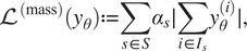 $$ {\mathrm{\mathcal{L}}}^{\left(\mathrm{mass}\right)}\left({y}_{\theta}\right):= \sum \limits_{s\in S}{\alpha}_s\mid \sum \limits_{i\in {I}_s}{y}_{\theta}^{(i)}\mid, $$
where
 $ S $
is the set of different species and
$ S $
is the set of different species and
 $ {I}_s $
is the indices for a specific species
$ {I}_s $
is the indices for a specific species
 $ s $
. The parameters
$ s $
. The parameters
 $ {\alpha}_i $
need to be tuned, chosen too small the mass violation will not be decreased, if a factor is too large, the network can find the local optimum that is constantly zero, the values can be found in the Supplementary Material. The other term penalizes negative mass values and is given byFootnote
2
$ {\alpha}_i $
need to be tuned, chosen too small the mass violation will not be decreased, if a factor is too large, the network can find the local optimum that is constantly zero, the values can be found in the Supplementary Material. The other term penalizes negative mass values and is given byFootnote
2
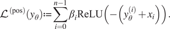 $$ {\mathrm{\mathcal{L}}}^{\left(\mathrm{pos}\right)}\left({y}_{\theta}\right):= \sum \limits_{i=0}^{n-1}{\beta}_i\mathrm{ReLU}{\left(-\left({y}_{\theta}^{(i)}+{x}_i\right)\right)}. $$
Using a ReLU function, all negative values are getting penalized. In our case
 $ n\hskip0.35em =\hskip0.35em 28 $
,
$ n\hskip0.35em =\hskip0.35em 28 $
,
 $ {x}_i $
is the corresponding full input variable to predicted tendency
$ {x}_i $
is the corresponding full input variable to predicted tendency
 $ {y}_{\theta}^{(i)} $
. The factors
$ {y}_{\theta}^{(i)} $
. The factors
 $ {\beta}_i $
need to be tuned, similar to
$ {\beta}_i $
need to be tuned, similar to
 $ {\alpha}_i $
.
$ {\alpha}_i $
.
2.3.2. Hard constraining
In order to have a guarantee for mass conservation or positive masses, we implement a correction and a completion method. This is done at test time as an additional network layer, a version where this is implemented within the training of the NN did not improve the performance.
Inequality correction. For the correction method, predicted values that result in an overall negative mass or number are set to a value such that the full value is zero. For the NNs intermediate output
 $ {\tilde{y}}_{\theta } $
, the final output is given by:
$ {\tilde{y}}_{\theta } $
, the final output is given by:
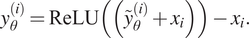 $$ {y}_{\theta}^{(i)}=\mathrm{ReLU}\left(\left({\tilde{y}}_{\theta}^{(i)}+{x}_i\right)\right)-{x}_i. $$
Equality completion. The completion method addresses mass violation, for each species one variable’s prediction is replaced by the negative sum of the other same species’ tendencies. We obtained the best results by replacing the worst-performing variable. This completion results in exact mass conservation. For a species
 $ S $
, we choose index
$ S $
, we choose index
 $ j\in {I}_S $
, the completion layer is defined as follows:
$ j\in {I}_S $
, the completion layer is defined as follows:
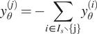 $$ {y}_{\theta}^{(j)}=-\sum \limits_{i\in {I}_s\backslash \left\{j\right\}}{y}_{\theta}^{(i)} $$
3. Results
3.1. Predictive performance
3.1.1. Metrics
We consider multiple metrics to get an insight into the performance of the different emulator designs, covering overall predictive accuracy, mass violation, and predicting nonphysical values. We look at the
 $ {R}^2 $
score and the MSE. To understand mass violation, we look at the mass biases for the different species and the overall mass violation, where all scores are normalized by the mean over the respective species. The metrics are completed with two scores about negative value predictions: An overall fraction of negative and therefore nonphysical predictions and the average negative extend per predicted value. For all the different scores and architectures, we take the mean over five different random initializations of the underlying NN.
$ {R}^2 $
score and the MSE. To understand mass violation, we look at the mass biases for the different species and the overall mass violation, where all scores are normalized by the mean over the respective species. The metrics are completed with two scores about negative value predictions: An overall fraction of negative and therefore nonphysical predictions and the average negative extend per predicted value. For all the different scores and architectures, we take the mean over five different random initializations of the underlying NN.
3.1.2. Evaluation and comparison
In Table 1, we display the scores for our emulator variants. We achieve good performance with a 77.1%
 $ {R}^2 $
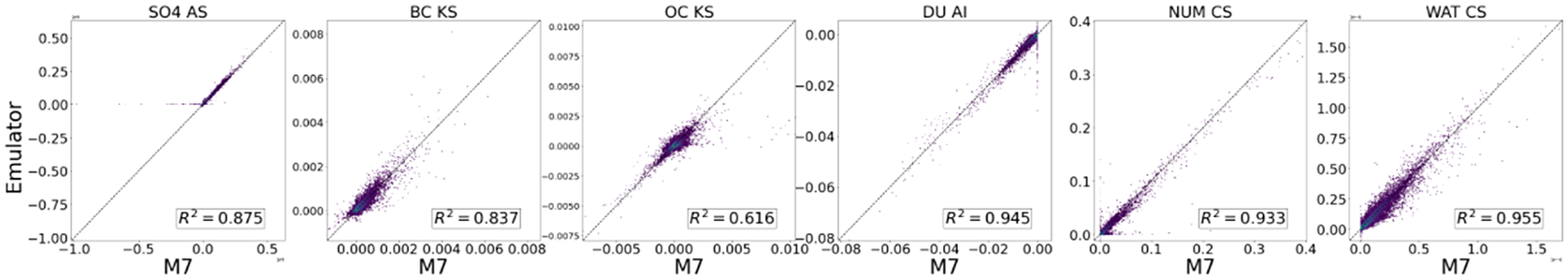
score and an MSE of 0.16. Using the correction method results per construction in no negative predictions, but increases the mass violation. The accuracy scores are not negatively affected by the correction operation. With the completion method, we achieve perfect mass conservation and a very slight worsening of the other metrics. The mass regularization decreases the overall mass violation and decreases the mass biases for most cases. The positivity loss term decreases the negative fraction and negative mean by a large amount. A few examples are plotted in Figure 2. In overall, the architecture with an additional correction procedure could be a good choice to use in a GCM run, having the guarantee of no negative masses and good accuracy in the original units. The mass violation is relatively low for all cases.
$ {R}^2 $
score and an MSE of 0.16. Using the correction method results per construction in no negative predictions, but increases the mass violation. The accuracy scores are not negatively affected by the correction operation. With the completion method, we achieve perfect mass conservation and a very slight worsening of the other metrics. The mass regularization decreases the overall mass violation and decreases the mass biases for most cases. The positivity loss term decreases the negative fraction and negative mean by a large amount. A few examples are plotted in Figure 2. In overall, the architecture with an additional correction procedure could be a good choice to use in a GCM run, having the guarantee of no negative masses and good accuracy in the original units. The mass violation is relatively low for all cases.
Test metrics for different architectures and transformations.
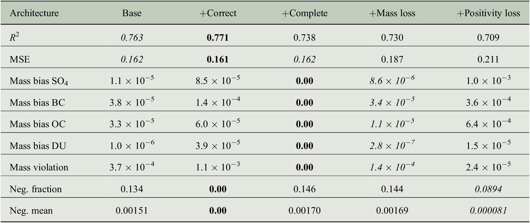
Note. Base means the usage of only the base NN, correct adds the correction procedure and complete the completion procedure. Mass reg. and positivity reg. include the regularization terms. Best scores are in bold and second-best scores are in italics.
Abbreviations: BC, black carbon; DU, dust; OC, primary organic carbon; SO4, sulfate.
This figure shows the test prediction of our emulators against the true M7 values. For each type (species, number particles, and water), we plot the performance of one variable (using the median or worse performing, see all in Supplementary Material).
Although the emulator performs well in an offline evaluation, it still remains to be shown how it performs when implemented in the GCM and runs for multiple time steps. Good offline performance is not necessarily a guarantee for good online performance (Rasp, Reference Rasp2020) in the case of convection parameterization, where a model crash could occur. In our case, it is likely that offline performance is a good indicator of online performance, as a global climate model crash is not expected because aerosols do not strongly affect large-scale dynamics.
3.2. Runtime
We conduct a preliminary runtime analysis by comparing the Python runtime for the emulator with the Fortran runtime of the original aerosol model. We take the time for one global time step, which is about 570,392 data points to predict. For the M7 model, the 31 vertical levels are calculated simultaneously and for the emulator, we predict the one-time step at once, using a batch size of 571,392 and taking into account the time for transforming variables and moving them on and off the GPU. We use a single NVIDIA Titan V GPU and a single Intel Xeon 4108 Central processing unit (CPU). As shown in Table 2, we can achieve a large speed-up of over 11,000× in a pure GPU setting. Including the time it takes to move the data from the CPU onto the GPU and back the acceleration is 64 times faster compared to the original model. In case of no available GPU, the NN emulator is still 2.8 times faster. Here, further speed-ups will be achieved by using multiple CPUs, a smaller network architecture, and efficient implementation in Fortran.
Runtime comparison for the original M7 model and the NN emulator.
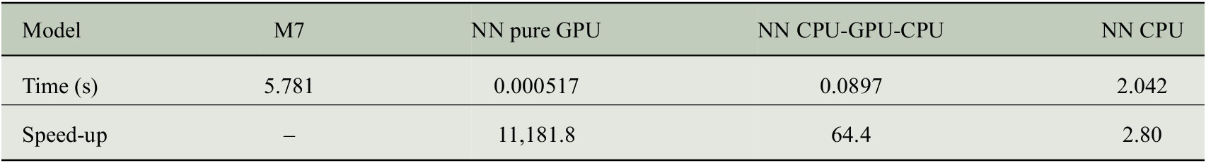
Note. NN pure GPU includes only the transformation of the variables and the prediction, whereas NN CPU-GPU-CPU also includes the time to transfer the data from the CPU to the GPU and back to the CPU.
Abbreviation: NN, neural network.
4. Conclusion and Future Work
To enable accurate climate forecasts aerosols need to be modeled with lower computational costs. This work shows how NNs can be used to learn the mapping of an aerosol microphysics model and how simple the physical constraints can be included in the model. Our neural models approximate the log-transformed tendencies excellently and the original units’ tendencies well. On the test set, an overall regression coefficient of 77.1% as well as an MSE of 16.1% is achieved. Using a GPU, we accomplish a large speed-up of 11,181 times faster compared to the original M7 model in a pure GPU setting, with the time to move from and to the CPU we are still significantly faster having a speed-up factor of 64. On a single CPUm, the speed-up is 2.8 times faster. By adding completion and correction mechanisms, we can remove mass violation or negative predictions completely and make our emulator feasible for stable a GCM run.
How much of a speed-up can be achieved in the end remains to be shown, when the machine learning model is used in a GCM run. Different versions of our emulator need to be run within the global climate model to show which setup performs the best online. A further step would be the combination of the different methods for physics constraining, to achieve both mass conservation and mass positivity at the same time.
Author Contributions
Conceptualization: P.H., P.S., J.K., D.W.-P., N.R.G.; Data curation: D.W.-P., P.H., D.S.; Data visualization: P.H.; Methodology: P.H.; Writing original draft: P.H. All authors approved the final submitted draft.
Competing Interests
The authors declare no competing interests exist.
Data Availability Statement
The code for this neural network emulator can be found at https://github.com/paulaharder/aerosol-microphysics-emulation. The data used for this work is available at https://zenodo.org/record/5837936.
Ethics Statement
The research meets all ethical guidelines, including adherence to the legal requirements of the study country.
Funding Statement
D.W.-P. and P.S. acknowledge funding from NERC projects NE/P013406/1 (A-CURE) and NE/S005390/1 (ACRUISE). D.W.-P. and P.S. also acknowledge funding from the European Union’s Horizon 2020 research and innovation program iMIRACLI under Marie Skłodowska-Curie grant agreement no. 860100. P.S. additionally acknowledges support from the ERC project RECAP and the FORCeS project under the European Union’s Horizon 2020 research program with grant agreements 724,602 and 821,205.
Provenance
This article is part of the Climate Informatics 2022 proceedings and was accepted in Environmental Data Science on the basis of the Climate Informatics peer review process.
Supplementary Materials
To view supplementary material for this article, please visit http://doi.org/10.1017/eds.2022.22.


 Open access