


Impact Statement
Extreme rainfall events significantly impact society, ecosystems, and the economy. Developing reliable, locally-relevant information about extremes is critical for building actionable adaptation and mitigation strategies. Statistical downscaling using machine learning algorithms has attracted the attention of researchers for its ability to provide downscaled high-resolution precipitation data at a much lower computational cost than dynamical downscaling. The present study applies a set of deep learning models to rapidly perform 8× downscaling of hourly precipitation data. Our best model outperforms existing deep learning models in reproducing the localised spatial variability of mean and extreme precipitation. Our model can rapidly produce multiple ensemble members of high-resolution precipitation data with reasonable accuracy and with less computational cost, allowing us to better characterise precipitation extremes.
1. Introduction
Spatially downscaling precipitation from coarse resolution datasets and model outputs (~100’s of kms) to local scale resolution (~10’s of kms or less) allows for a more accurate representation of the spatial variability at fine scales. For climate projections, this will be useful for developing region-specific climate adaptation strategies. For these purposes, recent deep learning methods, especially, the super-resolution approaches, are being widely used for empirical precipitation downscaling (Vandal et al., Reference Vandal, Kodra, Ganguly, Michaelis, Nemani and Ganguly2017; Harilal et al., Reference Harilal, Singh and Bhatia2021; Kumar et al., Reference Kumar, Chattopadhyay, Singh, Chaudhari, Kodari and Barve2021; Chandra et al., Reference Chandra, Sharma and Mitra2022; Wang et al., Reference Wang, Tian and Carroll2023). In precipitation downscaling, super-resolution models are trained to learn the relationship between the coarse-scale precipitation data and the fine-scale precipitation data, and then apply this relationship to generate high-resolution precipitation maps. These super-resolution deep learning models are computationally efficient and relatively fast compared to traditional dynamical downscaling.
Previous studies have developed super-resolution-based deep learning models for precipitation downscaling using a convolutional neural network (CNN) (Vandal et al., Reference Vandal, Kodra, Ganguly, Michaelis, Nemani and Ganguly2017; Chandra et al., Reference Chandra, Sharma and Mitra2022; Wang et al., Reference Wang, Tian and Carroll2023). For example, Vandal et al. (Reference Vandal, Kodra, Ganguly, Michaelis, Nemani and Ganguly2017) used the super-resolution CNN (SRCNN) model architecture (Dong et al., Reference Dong, Loy, He and Tang2014) and applied it to the precipitation downscaling by introducing orography as an auxiliary input to the model and named it DeepSD. They showed that DeepSD outperformed the commonly used empirical downscaling techniques like bias correction spatial disaggregation (BCSD) for precipitation downscaling (for a downscale factor of 8) across the United States for grid point-based metrics such as mean bias, root mean square error, and correlation coefficient. Work with DeepSD showed that providing orography as an additional input enhances the accuracy of model output based on grid point metrics (Vandal et al., Reference Vandal, Kodra, Ganguly, Michaelis, Nemani and Ganguly2017; Kumar et al., Reference Kumar, Chattopadhyay, Singh, Chaudhari, Kodari and Barve2021). However, it is not clearly shown that adding orography improves the fine-scale spatial variability of downscaled precipitation products from coarse to a fine grid. Recently, Wang et al. (Reference Wang, Tian and Carroll2023) developed super-resolution deep residual network models with customised loss functions to downscale the hourly precipitation data (for a downscale factor of 12) over the northern region of the Gulf of Mexico and showed their model performs better than the quantile mapping based empirical downscaling technique. In these previous studies, super-resolution deep learning models are mostly based on CNNs. CNNs are mainly used for feature extraction and in these CNN-based models, upscaling is performed using interpolation techniques (with fixed parameters). Unlike CNNs, deconvolution (or transposed convolution) neural networks (DNs) are used for reconstruction purposes and upscaling is done with learnable parameters. In this study, we develop DN-based model architecture for the downscaling of hourly precipitation data over the Australian region. Further, we provided the orographic information at various steps (2, 4, and 8×) of resolution improvement in the DN model to systematically assess the influence of the additional orographic information on the precipitation downscaling. We compare our DN models with the baseline DeepSD model and evaluate the ability of deep learning models to reconstruct the fine spatial scale structure of hourly precipitation from its coarse resolution product.
2. Data
For this study, we use high-quality modern reanalysis output dynamically downscaled to fine resolution using the Conformal Cubic Atmospheric Model (CCAM) (McGregor and Dix, Reference McGregor and Dix2008). This creates a “model as truth” or “perfect model” exercise to rigorously assess the deep learning models. Output is high-resolution (at 12.5 km) hourly precipitation data and static orography data over the Australian region from 1980 to 2020. The ERA5 reanalysis data (Hersbach et al., Reference Hersbach, Bell, Berrisford, Hirahara, Horányi, Muñoz-Sabater, Nicolas, Peubey, Radu, Schepers, Simmons, Soci, Abdalla, Abellan, Balsamo, Bechtold, Biavati, Bidlot, Bonavita, de Chiara, Dahlgren, Dee, Diamantakis, Dragani, Flemming, Forbes, Fuentes, Geer, Haimberger, Healy, Hogan, Hólm, Janisková, Keeley, Laloyaux, Lopez, Lupu, Radnoti, de Rosnay, Rozum, Vamborg, Villaume and Thépaut2020) drives the CCAM model. These high-resolution data are conservatively averaged by a scale factor of 8 to 100 km coarse resolution. Deep learning models are trained using data from 1980 to 2012 (until September 15, 2012) and tested on data from 2012 (from September 16, 2012) to 2020. This data split between training and test sets is based on the commonly used 80–20 split rule and allows us to effectively scale over multiple nodes with proper load balance. We have normalized precipitation and orography input data using the training period’s maximum and minimum values. For the SRDN models, the normalization is scaled to 100 so that all the values are in the range of 0 to 100. We have adopted this normalization scheme because most of the hourly precipitation values are small and normalizing them to 0–1 produces a training dataset of nearly all zero values. For the DeepSD model, precipitation is scaled from 0 to 100 and orography from 0 to 1 because our solutions with scaling orography from 0 to 100 produce noisy results (not shown).
3. Methods
3.1. DeepSD
DeepSD is built by stacking the three separate SRCNN models (SRCNN1, SRCNN2, and SRCNN3) with orography as an additional input at every step of the resolution enhancement (Vandal et al., Reference Vandal, Kodra, Ganguly, Michaelis, Nemani and Ganguly2017). Each SRCNN model performs 2× resolution enhancement. For example, the SRCNN1 model takes in low-resolution precipitation input at 100 km, interpolates (bicubic) to 50 km, and uses orography at 50 km as a secondary input and then performs convolution operations and outputs the precipitation at 50 km. Both the 100 km input and 50 km target precipitation data for training the SRCNN1 model are produced by conservatively averaging the 12.5 km precipitation data. SRCNN1 has three convolution layers, layer-1 has 64 9 × 9 filters with a rectified linear unit (ReLU) non-linear activation, layer-2 has 32 1 × 1 filters with ReLU activation, and the last convolution layer has a 5 × 5 filter that linearly maps the previous layers 32 feature maps to the output.
The model architecture is the same for all three SRCNN models. Only the resolution of the input and target data differs between the three SRCNN models. SRCNN2 model is trained with 50 km precipitation and 25 km orography as inputs to output 25 km precipitation data. Similarly, SRCNN3 model is trained with 25 km precipitation and 12.5 km orography as inputs and outputs 12.5 km. For training purposes of SRCNN2 and SRCNN3, both the input and target precipitation data used for each model come from conservatively averaging the 12.5 km high-resolution CCAM data to the appropriate resolution.
In DeepSD, each SRCNN model is trained separately for 100 epochs with mean square error (MSE) as a loss function using the Adam optimizer (Kingma and Ba, Reference Kingma and Ba2015) with a learning rate of 1 × 10⁻⁴. The learning rate is further reduced by a factor of 0.1 to a minimum of 1 × 10⁻⁵ when the model stopped improving for at least 10 epochs. During prediction, all three SRCNN trained models are stacked together, that is, the SRCNN1 model output precipitation and associated high-resolution orography flow in as an input for the SRCNN2 and similarly SRCNN2 output with respective high-resolution orography is input for SRCNN3. We monitored the loss curve of training and testing data to ensure the model is not overfitting/underfitting the data. The loss curve of these models represents a good fit with no evidence we are overfitting the data (Figure 1).
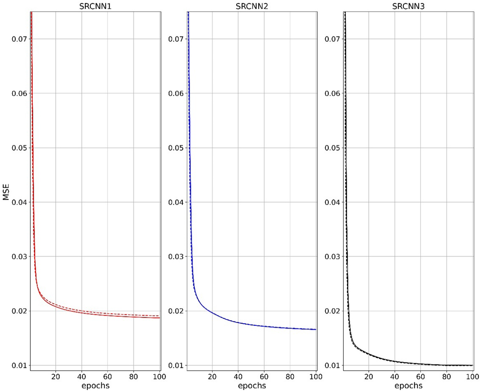
Figure 1. The DeepSD models’ (SRCNN1, SRCNN2, and SRCNN3) MSE computed from training (solid line) and test (dashed line) normalized datasets during the model training process over 100 epochs. The MSE values shown are calculated using the normalized data. To estimate the MSE of DeepSD, we need to stack the three models together. Hence the errors in panel (a) flow to panel (b), and the errors in panel (b) flow to panel (c), which leads to model prediction with greater MSE than what is shown in panel (c). The MSE of DeepSD is summarized in Table 1.
3.2. SRDN
Our super-resolution DN (SRDN) model is primarily built on deconvolution layers. It has three main deconvolution layers; each consists of 64 7 × 7 filters with ReLU non-linear activation and a convolution layer at the end to linearly map the last deconvolution layer feature maps to the output. Each deconvolution layer does a 2× resolution enhancement. This model does a straight 8× resolution enhancement, which means it takes 100 km of precipitation as an input and outputs 12.5 km of precipitation. Guided by studies with DeepSD, we explored including orography as an additional input to the model in several ways.
We develop two models by providing orography at different stages of the model architecture. Version 1 adds to the SRDN by concatenating high-resolution (12.5 km) orography as a channel to the SRDN output high-resolution precipitation (12.5 km) and passing it through a convolution layer of 64 7 × 7 filters with ReLU activation and one other convolution layer at the end to linearly map previous layer 64 feature maps to the output. This model is named SRDN-O. Version two, called SRDN-SO, is built on the SRDN-O model by providing orography at multiple steps as feature maps (i.e., 50 km resolution orography is appended to the first deconvolution layer and 25 km resolution orography to the second deconvolution layer, respectively). All three models are trained with MSE as a loss function for 30 epochs using the Adam optimizer with a learning rate of 3 × 10⁻³. The learning rate is further reduced by a factor of 0.1 to a minimum of 1 × 10⁻⁵ when the model stopped improving for at least 10 epochs. The loss curve of these models represents a good fit with no evidence of overfitting the data (see Figure 2).
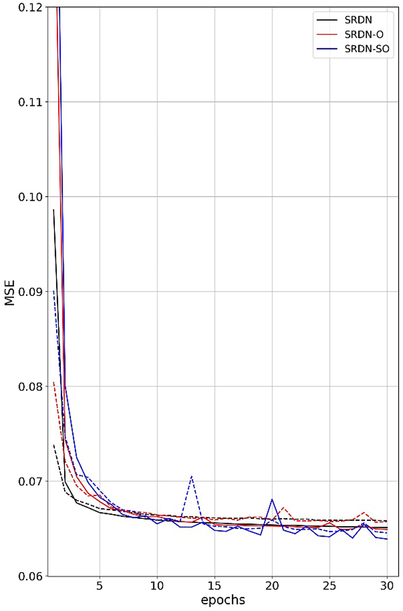
Figure 2. The SRDN models’ MSE error computed from training (solid line) and test (dashed line) normalized datasets during the model training process over 30 epochs. The MSE values shown are calculated using the normalized data.
All the models considered in this study are developed using the TensorFlow (Abadi et al., Reference Abadi, Agarwal, Barham, Brevdo, Chen, Citro, Corrado, Davis, Dean, Devin, Ghemawat, Goodfellow, Harp, Irving, Isard, Jia, Jozefowicz, Kaiser, Kudlur, Levenberg, Mane, Monga, Moore, Murray, Olah, Schuster, Shlens, Steiner, Sutskever, Talwar, Tucker, Vanhoucke, Vasudevan, Viegas, Vinyals, Warden, Wattenberg, Wicke, Yu and Zheng2015) and Keras (Chollet et al., Reference Chollet2015) application programming interfaces and trained in a distributed training framework using the Horovod package (Sergeev and Del Balso, Reference Sergeev and Del Balso2018). These models are trained on 80 Nvidia V100 GPUs with 32 GB memory at the National Computational Infrastructure in Canberra on the Gadi supercomputer.
4. Results
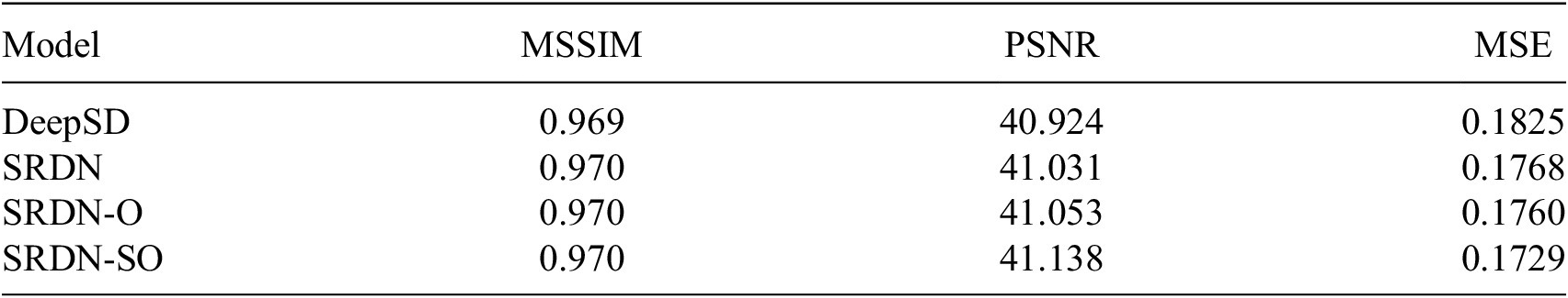
First, we compare the model’s performance based on standard metrics (peak signal-to-noise ratio [PSNR] and mean structural similarity index measure [MSSIM]) of image resolution enhancement models in computer vision applications. The PSNR and MSSIM are calculated for each predicted precipitation map and are averaged over all test data samples to compute their mean (shown in Table 1). The MSSIM results suggest that all the models perform similarly. The mean PSNR suggests that the SRDN-SO model performs slightly better than the other models in this study in enhancing the resolution of the hourly precipitation field at a downscale factor of 8 (100 to 12.5 km). However, these standard metrics are similar across the models used and are insufficient to identify the best deep-learning model. To quantitatively assess the ability of the deep learning models to reconstruct the 12.5 km from the 100 km precipitation data, we used 2D spatial Fourier Transforms analysis. We compute the predicted precipitation map’s power spectral density (PSD) and compare it with PSD of the target precipitation (Manepalli et al., Reference Manepalli, Singh, Mudigonda, White and Albert2020; Kashinath et al., Reference Kashinath, Mustafa, Albert, Wu, Jiang, Esmaeilzadeh, Azizzadenesheli, Wang, Chattopadhyay, Singh, Manepalli, Chirila, Yu, Walters, White, Xiao, Tchelepi, Marcus, Anandkumar, Hassanzadeh and Prabhat2021). Looking at only PSD may provide misleading conclusions when the predicted data are noisy. Hence, we also examine the spatial maps qualitatively to gauge how well the model predictions are representing the precipitation data.
Table 1. Comparison of mean peak signal-to-noise ratio (PSNR), mean structural similarity index measure (MSSIM), and mean square error (MSE) of predicted precipitation during test period between different models
First, the PSD is calculated for each of the predicted precipitation maps and averaged over all time samples to get the mean PSD. The diagonal of one quadrant (symmetrical across quadrants) of the mean PSD is shown in Figure 3. All the considered models show less power than the target data at short wavelengths. The DeepSD model’s PSD drops substantially more at the short wavelength (around 50 km) than the SRDN models. SRDN-SO model shows slightly more power in both mid-range and short wavelengths than the other models. The additional use of the orography at each step of resolution enhancement appears to improve the model representation of the spatial variability. However, the effect is likely to be even more notable over mountain ranges than minor orographic regions, and this effect may be washed out in this domain statistic, so next, we examine spatial maps.
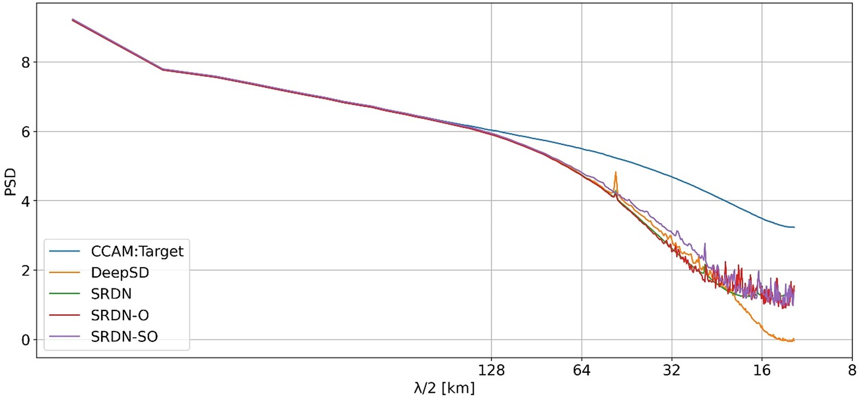
Figure 3. The diagonal of one of the quadrants (all quadrants are symmetrical) of mean spatial PSD of the hourly precipitation field versus wavelength (λ) using the target data and the models’ predicted output during the test period.
Figure 4 shows the climatology rainfall with zoomed-in plots in two regions with complex orography (i.e., Papua New Guinea [PNG] and Southeast Australia [SEA]). On average, SRDN-SO captures the mean well (Figure 4a vs. b). At large scale, all deep learning models are quite effective in representing the mean rainfall (figure not shown). If we zoom in on the two regions (PNG and SEA), we start to see the differences between the models and the benefit of orography. It can be visually seen that the SRDN-SO model performs well in reconstructing the spatial structure over complex orographic regions of PNG (Figure 4c–g) and SEA (Figure 4h–l) compared to other models. To quantify the subtle spatial differences between the deep learning models, we show the PSD of climatology rainfall (Figure 4m). The PSDs of SRDN-O and SRDN-SO models closely match the target PSD at mid-range wavelengths; however, they slightly overestimated at short wavelength space.
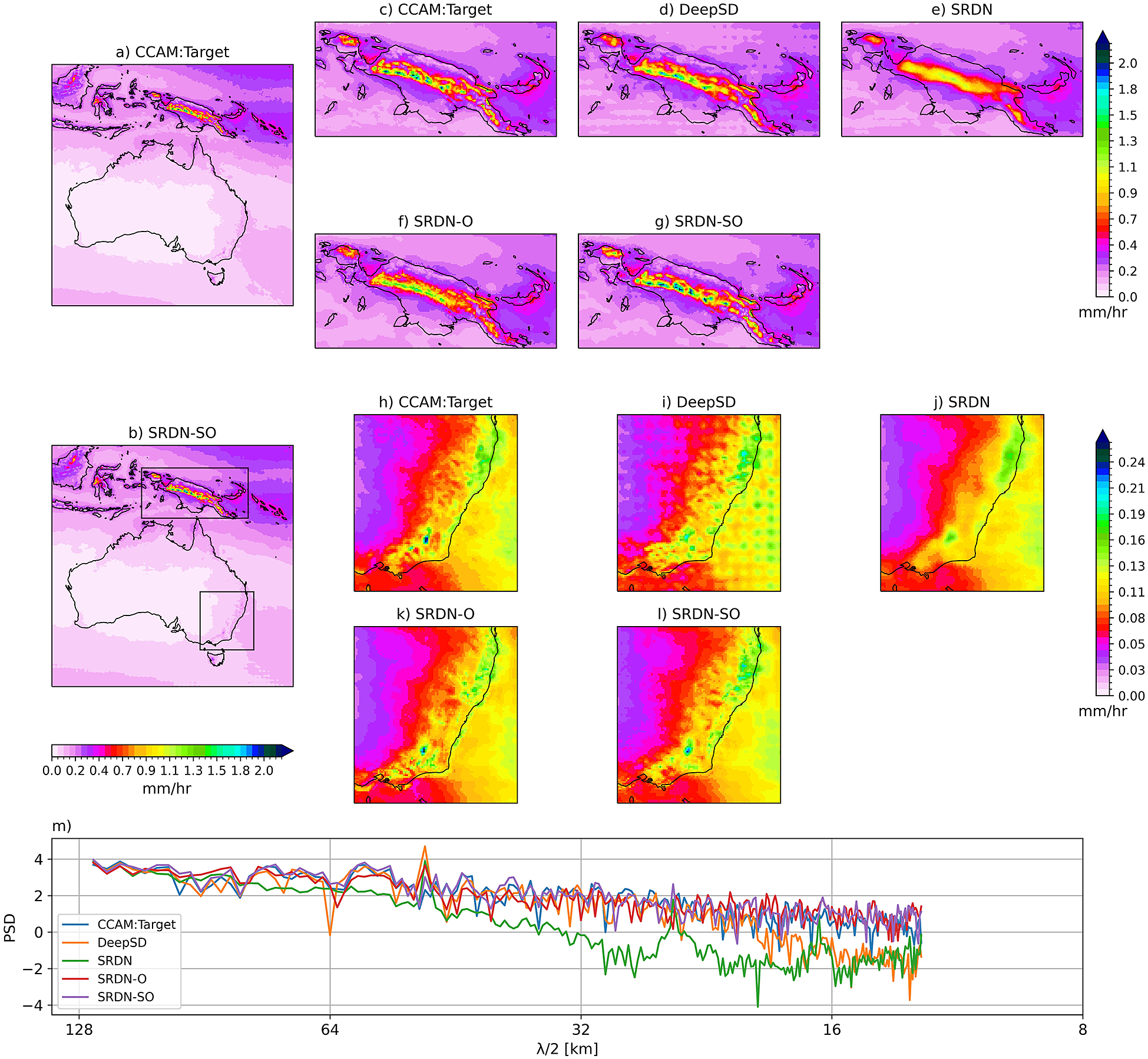
Figure 4. Hourly precipitation climatology over the study region of target (a) and SRDN-SO model (b) predictions during the test period. The top panels (c–g) and middle panels (h–l) show climatology over zoomed-in regions of Papua New Guinea and southeast Australia, respectively. The bottom panel (m) line plot shows the PSD (shown only for mid-range and short wavelengths) of the climatology of the whole domain for different considered models and the target.
Figure 5 shows the 95th percentile plot and the respective PSD of the models and target data. On a domain scale, SRDN-SO predicts the 95th percentile well (Figure 5a vs. b). Further, SRDN-SO model extracts the fine-scale spatial structure and magnitude of the 95th percentile precipitation field much better than other models, particularly over the PNG (Figure 5c–g) and SEA (Figure 5h–l) regions. However, the SRDN-SO model underestimates the PSD of the 95th percentile precipitation compared to the target data (Figure 5m). An important note on these results is that all the deep learning models underestimate the target 99th percentile extreme value (not shown). This may be due to the lower sampling size at the extremes of the distribution and structural model features of CCAM that cannot be replicated by deep learning models. We plan to investigate this further.
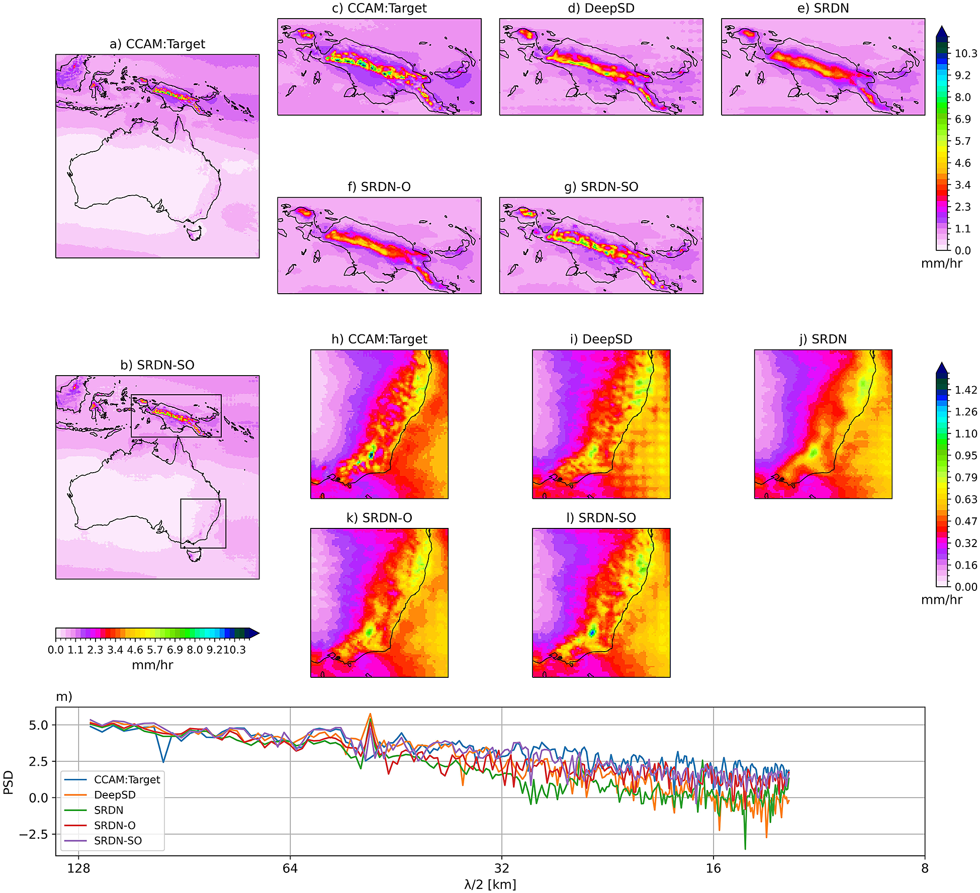
Figure 5. The 95th percentile hourly precipitation for the target (a) and SRDN-SO model (b) predictions during the test period. The top panels (c–g) and middle panels (h–l) show Papua New Guinea and southeast Australia, respectively. The bottom panel (m) line plot shows the corresponding PSD of the target and the deep-learning models.
5. Conclusion
In this study, we have developed an SRDN model architecture for rapidly downscaling the hourly precipitation by a scale factor of 8 (100 to 12.5 km) over the Australian region that successfully downscales precipitation to accurately reproduces the mean and extreme (95th percentile). We systematically evaluated the use of orography to generate the downscaled precipitation. By utilizing orography at multiple resolution steps, we improved the model’s ability to reconstruct the fine-scale spatial variability of precipitation of both the mean and extreme (95th percentile). Our SRDN-SO model outperforms a previously used deep-learning model (DeepSD) with better skill in reproducing the fine-scale spatial structure of both the climatology and the extremes. This model architecture can be applied to different regions for downscaling hourly precipitation.
The proposed SRDN-SO model has huge potential to rapidly downscale hourly precipitation products from various global climate models ensemble members dynamically downscaled by a coarse resolution CCAM to high resolution with less computational cost than straight dynamical downscaling to the desired resolution. This can help produce large ensembles of high-resolution precipitation data needed to characterizing extreme rainfall events. The results here also illustrate the benefits of systematic assessment and evaluation of the results of deep learning models, and we suggest that this should become a more routine part of analysis using deep learning models for downscaling. However, there are a few limitations to our proposed SRDN-SO model. The model cannot accurately represent the PSD at short wavelengths compared to the target data. Several recent studies show models based on Generative Adversarial Networks (GANs), particularly Enhanced Super-Resolution GAN (ESRGAN; Wang et al., Reference Wang, Yu, Wu, Gu, Liu, Dong, Loy, Qiao, Tang, Leal-Taixé and Roth2019) models can accurately represent the PSD even at short wavelengths in wind field for downscaling by a factor of 2 and 4 (Singh et al., Reference Singh, White and Albert2019; Manepalli et al., Reference Manepalli, Singh, Mudigonda, White and Albert2020; Kashinath et al., Reference Kashinath, Mustafa, Albert, Wu, Jiang, Esmaeilzadeh, Azizzadenesheli, Wang, Chattopadhyay, Singh, Manepalli, Chirila, Yu, Walters, White, Xiao, Tchelepi, Marcus, Anandkumar, Hassanzadeh and Prabhat2021). However, these previous studies are based on downscaling winds by a factor of 2 and 4, and not precipitation downscaling by a factor 8. The power spectrum of wind maps is expected to differ from precipitation maps because of the more sporadic and chaotic nature of the precipitation (particularly, convective precipitation), making precipitation downscaling to finer spatial scales more challenging. Hence, based on the previous studies, we cannot be definite that ESRGAN could accurately represent the PSD for precipitation downscaling of a downscale factor of 8 (100 to 12.5 km). This needs to be further examined in future work. Following the RainNet initiative of providing the precipitation dataset for deep learning-based downscaling (Chen et al., Reference Chen, Feng, Liu, Ni, Lu, Tong and Liu2022), we will make the data set available as a precipitation downscaling benchmark for the Oceania region and encourage downscaling practitioners to apply their models to this data. In future precipitation downscaling we will assess the benefit of additional input variables such as geopotential height, wind speed, and direction, and explore the inclusion of temporal dependency in the model based on the Chen et al. (Reference Chen, Feng, Liu, Ni, Lu, Tong and Liu2022) approach.
Acknowledgments
We would like to thank National Computing Infrastructure (NCI) Australia for providing computational resources. We also thank TensorFlow, Keras, and Horovod teams for openly providing their APIs.
Author contribution
Conceptualization: P.J.R., R.M., J.T.; Formal analysis: P.J.R; Methodology: P.J.R., R.M., J.T., M.T., M.G.; Writing–original draft: P.J.R; Writing–review & editing: R.M., J.T., M.T., M.G.
Competing interest
The authors declare no competing interests exist.
Data availability statement
ERA5 data used to drive the CCAM downscaling is freely available at: https://doi.org/10.24381/cds.bd0915c6. The high-resolution CCAM data can be made available upon request to the corresponding author.
Funding statement
The authors would like to acknowledge the funding support of the CSIRO and Australian Climate Service.
Provenance statement
This article is part of the Climate Informatics 2023 proceedings and was accepted in Environmental Data Science on the basis of the Climate Informatics peer review process.


 Open access