


Impact Statement
The dynamics of the oceans are a key issue to understand the climate system, as they transport heat from equatorial areas to colder ones. Ocean currents are therefore an important variable, and their estimation requires to measure the sea surface height (SSH). This altimetry map is hard to acquire in practice and thus has a low effective resolution compared to other physical data such as the sea surface temperature (SST). In this work, we propose a deep learning algorithm that takes advantage of the high-resolution information of the SST to enhance the resolution of the SSH.
1. Introduction
The oceans, with their massive heat storage capacity and conveyor belt circulation, are the prime drivers of climate regulation. Better understanding and monitoring their response to climate change requires high-resolution data sets. Such data sets are usually obtained by satellite imaging, numerical modeling, or by a combination of the two through data assimilation (Bertino et al., Reference Bertino, Evensen and Wackernagel2003). Satellite remote sensing provides a multitude of geophysical data fields with various sampling in space and in time. For instance, sea surface temperature (SST) can be obtained at a very high resolution (1.1 and 4.4 km) from the AVHRR instruments (Emery et al., Reference Emery, Brown and Nowak1989). On the other hand, sea surface height (SSH) can be retrieved at a coarser resolution (around 25 km) from different satellites. SSH and SST variables are linked by a hidden physical relation (Leuliette and Wahr, Reference Leuliette and Wahr1999) that we aim to use by combining these multiresolution data to downscale the coarse SSH. This could lead to estimate ocean currents as they are formed by geostrophy from SSH gradient (Doglioni et al., Reference Doglioni, Ricker, Rabe and Kanzow2021). This is a super resolution (SR) problem applied to oceanography.
Since 2014 and the super resolution convolutional neural network (SRCNN) introduced by Dong et al. (Reference Dong, Loy, He, Tang, Fleet, Pajdla, Schiele and Tuytelaars2014), neural networks have been used to perform super resolution tasks, and often achieve state-of-the-art performances (Wang et al., Reference Wang, Chen and Hoi2021). A wide range of deep neural network architectures has been explored such as the residual networks (ResNet). ResNets allow the use of deeper architectures and bigger learning rates (Kim et al., Reference Kim, Lee and Lee2016; Lim et al., Reference Lim, Son, Kim, Nah and Lee2017). Various up-sampling strategies have also been tested such as the subpixel convolution method introduced by Shi et al. (Reference Shi, Caballero, Huszar, Totz, Aitken, Bishop, Rueckert and Wang2016a). However, the literature on super-resolution with deep learning networks focuses on lower upsampling factors, without multiresolution data. Therefore these methods should be adapted to the SSH downscaling problem because the network must be able to extract information from the high-resolution SST. This problem has been tackled by the RESAC neural network architecture (Thiria et al., Reference Thiria, Sorror, Mejia, Molines and Crepon2022), which is a proof-of-concept super-resolution architecture. Its main features are downscaling through consecutive resolutions, and using a cost function that monitors the correct downscaling in each of these resolutions. We propose a subpixel convolutional residual network, called RESACsub, a modified version of the RESAC network. As the RESAC network, RESACsub aims to downscale a low-resolution SSH using information from a higher-resolution SST. We achieve the SSH downscaling with a higher upsampling factor than in the RESAC proof of concept, but we only focused on the SSH, while RESAC also recovers the longitudinal and latitudinal velocities. In the following, we will present RESACsub, as well as its main differences from RESAC, briefly detail the data set used by both models, present the results obtained and discuss further potential developments.
2. Data
In order to train a supervised neural network as RESACsub, we need the data fields at every resolution. As SSH cannot be retrieved from a satellite at the resolution we want to downscale, we use simulated grided SSH and SST from an ocean physics-based model: NATL60 (Ajayi et al., Reference Ajayi, Le Sommer, Chassignet, Molines, Xu, Albert and Cosme2020). This model is based on the NEMO 3.6 (Madec et al., Reference Madec, Bourdallé-Badie, Bouttier, Bricaud, Bruciaferri, Calvert, Chanut, Clementi, Coward, Delrosso, Ethé, Flavoni, Graham, Harle, Iovino, Lea, Lévy, Lovato, Martin, Masson, Mocavero, Paul, Rousset, Storkey, Storto and Vancoppenolle2017) code, with atmospheric forcing, and initial conditions taken from MERCATOR (Lellouche et al., Reference Lellouche, Greiner, Le Galloudec, Regnier, Benkiran, Testut, Bourdalle-Badie, Drevillon, Garric, Drillet, Chassignet, Pascual, Tintoré and Verron2018). We use the SSH and SST state variables of this model at a very high resolution denoted R01 (for a resolution of 1/60° at the equator). At this resolution, the model has a very high running cost; therefore, we were only able to retrieve 1 year of training data (366 days starting from October 1, 2012), and 4 months of validation in 2008 (March, June, September, and December). We are well aware that we should use different test/validation dataset, but considering the importance of the annual cycle and that the main objective is to compare two models, we decided not to separate the four validation months. Compared to RESAC, our validation method is more rigorous as there cannot be data leakage from sampling the validation data from the training year.
We simulate the various resolutions by recursively averaging the pixels in a
 $ 3\times 3 $
mask. We then call, hereafter R01, R03, R09, R27, and R81, the five resolutions that we study with respective sizes at the grid center of (
$ 3\times 3 $
mask. We then call, hereafter R01, R03, R09, R27, and R81, the five resolutions that we study with respective sizes at the grid center of (
 $ 1.5\times 1.5 $
,
$ 1.5\times 1.5 $
,
 $ 4.5\times 4.5 $
,
$ 4.5\times 4.5 $
,
 $ 13\times 14 $
,
$ 13\times 14 $
,
 $ 40\times 41 $
, and
$ 40\times 41 $
, and
 $ 120\times 122\hskip0.24em {\mathrm{km}}^2 $
). We renormalize the data set between 0 and 1 to both stabilize the numerical calculations and equalize the importance of SST and SSH. In order to compare our models, we perform 10 rounds of training of each architecture, with different weight initialization on each training.
$ 120\times 122\hskip0.24em {\mathrm{km}}^2 $
). We renormalize the data set between 0 and 1 to both stabilize the numerical calculations and equalize the importance of SST and SSH. In order to compare our models, we perform 10 rounds of training of each architecture, with different weight initialization on each training.
3. Method
3.1. RESAC super-resolution method
In this paper, we compare two CNN architectures that use the same downscaling RESAC method. This method aims to learn the hidden link between a high-resolution SST and a low-resolution SSH. To that end, we progressively increase the resolution of our coarse SSH_R81 in three up-sampling steps each one with an up-sampling factor of 3 for a total up-sampling factor of 27. To perform each resolution increase we use a CNN block as shown in the RESAC method in Figure 1.
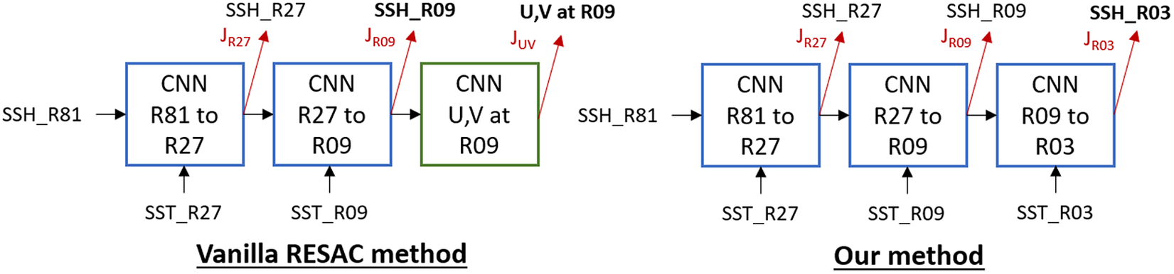
Figure 1. Comparison between the vanilla downscaling method used in Thiria et al. (Reference Thiria, Sorror, Mejia, Molines and Crepon2022) and this paper. The main two differences are that we increase the SSH resolution one step further but we do not retrieve the ocean circulation.
The Vanilla RESAC method as proposed by Thiria et al. (Reference Thiria, Sorror, Mejia, Molines and Crepon2022) performed only two downscaling CNNs starting from SSH_R81 (
 $ 120\times 122\hskip0.2em {\mathrm{km}}^2 $
) and retrieving SSH_R09 (
$ 120\times 122\hskip0.2em {\mathrm{km}}^2 $
) and retrieving SSH_R09 (
 $ 13\times 14\;{\mathrm{km}}^2 $
) for a total up-sampling factor of 9. But the original method also used another CNN block at the end of the network to compute the circulation (U and V currents) from the estimate SSH_R09. Our downscaling method upscales the SSH from
$ 13\times 14\;{\mathrm{km}}^2 $
) for a total up-sampling factor of 9. But the original method also used another CNN block at the end of the network to compute the circulation (U and V currents) from the estimate SSH_R09. Our downscaling method upscales the SSH from
 $ 120\times 122\;{\mathrm{km}}^2 $
down to
$ 120\times 122\;{\mathrm{km}}^2 $
down to
 $ 4.5\times 4.5\;{\mathrm{km}}^2 $
(upsampling factor of 27) without retrieving ocean currents. Both methods use cost functions that force the model to correctly downscale through the intermediary resolution. Therefore we use three loss functions at R27, R09, and R03 and the global loss of the model is their sum. The use of three separate loss functions guides the model to correctly reconstruct the intermediary resolutions, which depend on different physical phenomena given their scales. For each of these loss functions, we use mean squared error (MSE) between the estimated SSH and the target.
$ 4.5\times 4.5\;{\mathrm{km}}^2 $
(upsampling factor of 27) without retrieving ocean currents. Both methods use cost functions that force the model to correctly downscale through the intermediary resolution. Therefore we use three loss functions at R27, R09, and R03 and the global loss of the model is their sum. The use of three separate loss functions guides the model to correctly reconstruct the intermediary resolutions, which depend on different physical phenomena given their scales. For each of these loss functions, we use mean squared error (MSE) between the estimated SSH and the target.
In this work, every architecture uses the same downscaling method: a slightly different method than the one used by Thiria et al. (Reference Thiria, Sorror, Mejia, Molines and Crepon2022), which downscale SSH_R81 to SSH_R03 using every intermediate resolution SST without retrieving ocean currents. We denote this downscaling method as the RESAC method hereafter.
3.2. Network architecture
3.2.1. RESAC network
The original RESAC architecture upsamples the SSH with a bilinear upsampling and then applies
 $ Nloop $
times two convolution layers followed by a batch normalization (BN) layer as shown in Figure 2. In the following work, we set
$ Nloop $
times two convolution layers followed by a batch normalization (BN) layer as shown in Figure 2. In the following work, we set
 $ Nloop=5 $
, therefore, each downscaling CNN block has 10 convolution layers, each one with
$ Nloop=5 $
, therefore, each downscaling CNN block has 10 convolution layers, each one with
 $ 37 $
filters. We use the swish activation function for every convolution layer, except for the last one that uses a linear activation function.
$ 37 $
filters. We use the swish activation function for every convolution layer, except for the last one that uses a linear activation function.
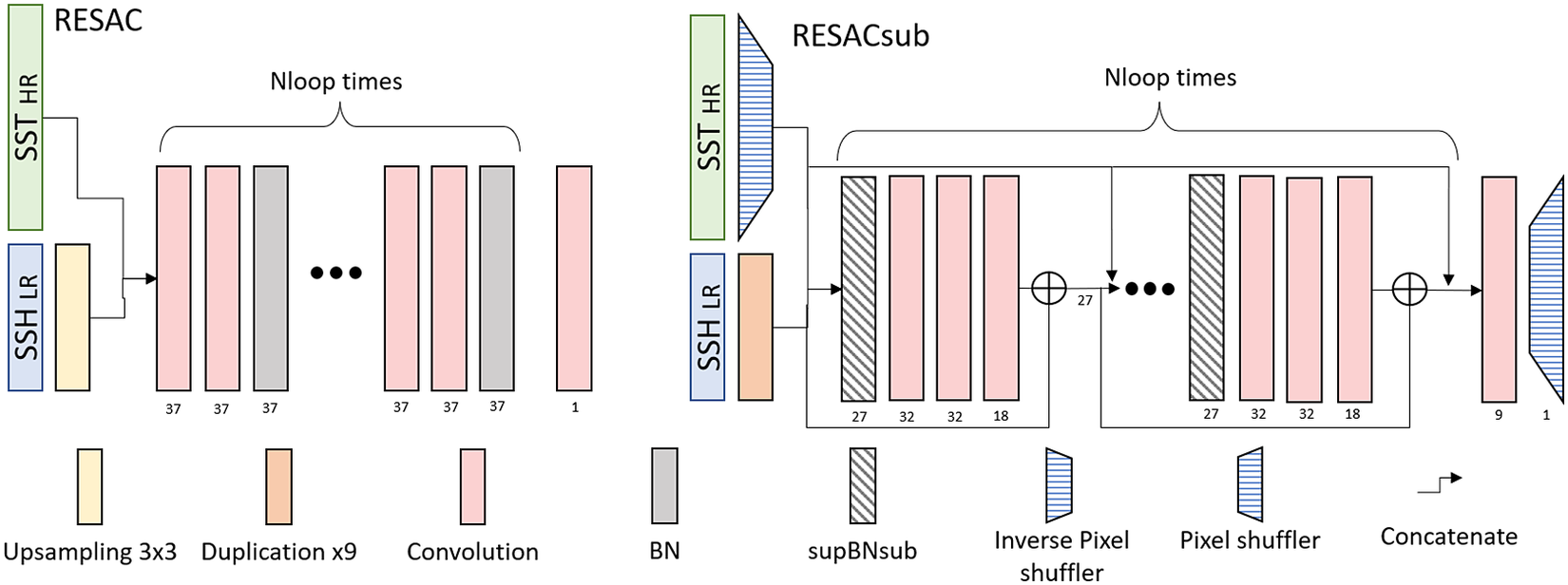
Figure 2. Comparison of the architectures of one downscaling step for RESAC and RESACsub. For each layer, the output number of channels is given below it.
3.2.2. RESACsub network
RESACsub is a Subpixel Convolutional Residual Network. It is a post-network upsampling strategy shown in Figure 2. The principle of a subpixel convolutional layer is to perform the convolution, not in the original image space (that we call supspace hereafter), but in a deeper and smaller space (that we call subspace hereafter). This method has been introduced by Shi et al. (Reference Shi, Caballero, Huszar, Totz, Aitken, Bishop, Rueckert and Wang2016a, Reference Shi, Caballero, Theis, Huszar, Aitken, Tejani, Totz, Ledig and Wang2016b): the upsampling is therefore performed at the end of the network by getting back to the supspace. The supspace is obtained from the subpsace by applying a pixel shuffler operation as shown in Figure 3. Two pixels that are spatial neighbors in the supspace are channel neighbors in the subspace. We call hereafter
 $ P $
the operation that transforms a subspace image into a supspace image and
$ P $
the operation that transforms a subspace image into a supspace image and
 $ {P}^{-1} $
the inverse operation, see equation (1):
$ {P}^{-1} $
the inverse operation, see equation (1):
 $$ {I}_{n,n,{R}^2c}^{sub}\underset{P^{-1}}{\overset{P}{\rightleftarrows }}{I}_{Rn, Rn,c}^{sup}, $$
where
 $ R $
is the upsampling factor (3 in our work),
$ R $
is the upsampling factor (3 in our work),
 $ n $
is the spatial dimension of the low-resolution image, and
$ n $
is the spatial dimension of the low-resolution image, and
 $ c $
is the number of channels. Therefore,
$ c $
is the number of channels. Therefore,
 $ {I}_{n,n,{R}^2c}^{sub} $
is the image in the subspace and
$ {I}_{n,n,{R}^2c}^{sub} $
is the image in the subspace and
 $ {I}_{Rn, Rn,c}^{sup} $
is the same image shifted in the supspace.
$ {I}_{Rn, Rn,c}^{sup} $
is the same image shifted in the supspace.
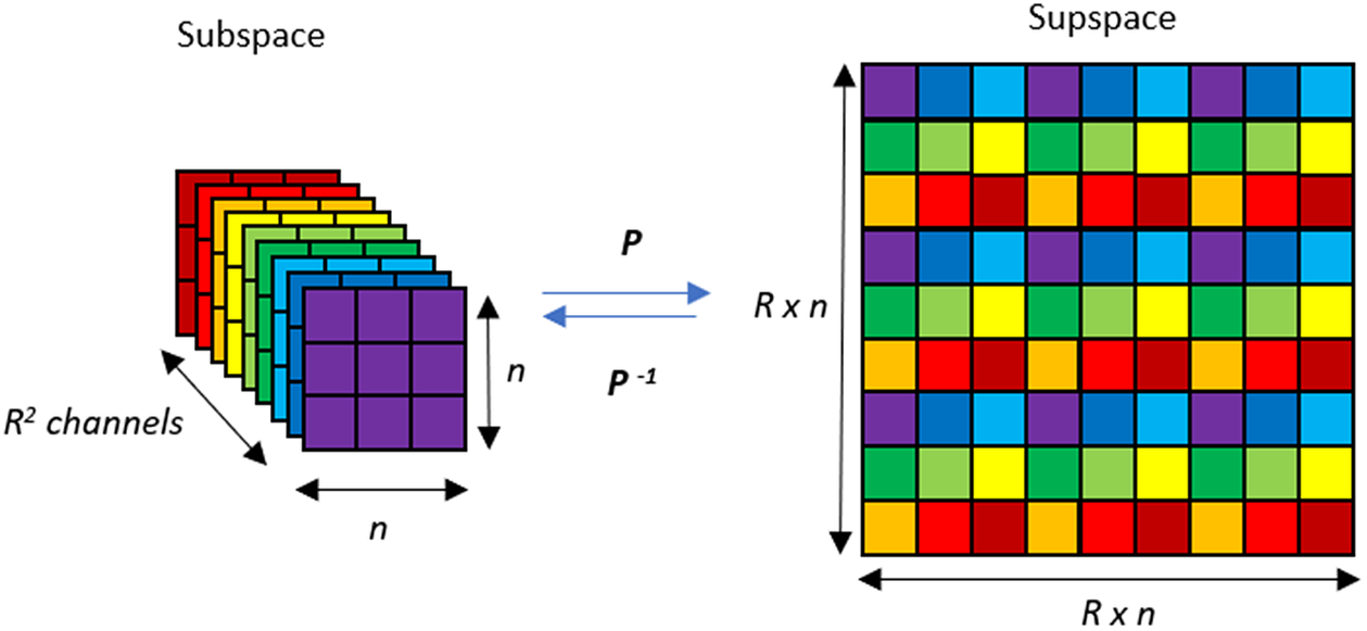
Figure 3. Pixel shuffler and inverse pixel shuffler.
In RESACsub we first concatenate the SST and the SSH in the subspace. As the SST is wider than the SSH, we first shift it to the subspace with an inverse pixel shuffling layer. To keep the same weight between SST and SSH images we duplicate nine times the low-resolution SSH image and concatenate the two images after doing so. We then use a Residual Network to downscale the SSH, with five residual loops (
 $ Nloop=5 $
). Each residual loop starts with an adapted form of BN that we detail in Section 3.2.3, followed by 3 convolution layers with respectively 32, 32, and 18 filters and the swish activation function. We then add the SSH and concatenate the SST. The final output layer is a convolution layer with nine filters and a linear activation function followed by a pixel shuffling.
$ Nloop=5 $
). Each residual loop starts with an adapted form of BN that we detail in Section 3.2.3, followed by 3 convolution layers with respectively 32, 32, and 18 filters and the swish activation function. We then add the SSH and concatenate the SST. The final output layer is a convolution layer with nine filters and a linear activation function followed by a pixel shuffling.
3.2.3. Batch normalization
With this subpixel convolution method, we use the channel dimension to store neighbors pixels and then perform a convolution layer. This implies that using BN will create strong checkerboard artifacts as each channel is normalized with a different mean and variance. The tests we performed confirmed this. To explain the impact of BN on the checkerboard artifacts, we must get back to the following equation:
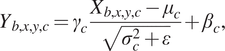 $$ {Y}_{b,x,y,c}={\gamma}_c\frac{X_{b,x,y,c}-{\mu}_c}{\sqrt{\sigma_c^2+\varepsilon }}+{\beta}_c, $$
where
 $ X $
and
$ X $
and
 $ Y $
are, respectively, the input and the output of the BN layer. They are four-dimensional tensors with
$ Y $
are, respectively, the input and the output of the BN layer. They are four-dimensional tensors with
 $ b $
as the batch coordinate,
$ b $
as the batch coordinate,
 $ x $
and
$ x $
and
 $ y $
as the two spatial coordinates of the image, and
$ y $
as the two spatial coordinates of the image, and
 $ c $
as the channel index. Parameters
$ c $
as the channel index. Parameters
 $ {\mu}_c $
and
$ {\mu}_c $
and
 $ {\sigma}_c $
are, respectively, the mean and the standard deviation of the image across the two space dimensions and the batch dimension for the channel
$ {\sigma}_c $
are, respectively, the mean and the standard deviation of the image across the two space dimensions and the batch dimension for the channel
 $ c $
. Finally,
$ c $
. Finally,
 $ \varepsilon $
is a small positive constant that we add for numerical stability,
$ \varepsilon $
is a small positive constant that we add for numerical stability,
 $ {\beta}_c $
and
$ {\beta}_c $
and
 $ {\gamma}_c $
are, respectively, the output mean and the output standard deviation that are learned during the training.
$ {\gamma}_c $
are, respectively, the output mean and the output standard deviation that are learned during the training.
The BN method thus learns the bias and the standard deviation of each channel independently during the training phase. This is inconsistent with the subpixel convolutional method because the channels do not represent different data or images, but neighbors pixels that have similar distributions and should be normalized the same way.
To fix this issue we use an adapted form of BN that we call
 $ \mathrm{supBNsub} $
as illustrated in Figure 4. Operator
$ \mathrm{supBNsub} $
as illustrated in Figure 4. Operator
 $ \mathrm{supBNsub} $
gets back to the supspace, applies a BN layer, and then returns to the subspace. If we call
$ \mathrm{supBNsub} $
gets back to the supspace, applies a BN layer, and then returns to the subspace. If we call
 $ BN $
the batch normalization operation described in Eq. (2), we can write the
$ BN $
the batch normalization operation described in Eq. (2), we can write the
 $ \mathrm{supBNsub} $
operator as
$ \mathrm{supBNsub} $
operator as
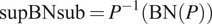 $$ \mathrm{supBNsub}={P}^{-1}\left(\mathrm{BN}(P)\right) $$
and SupBNsub method produces better results in RMSE sense.
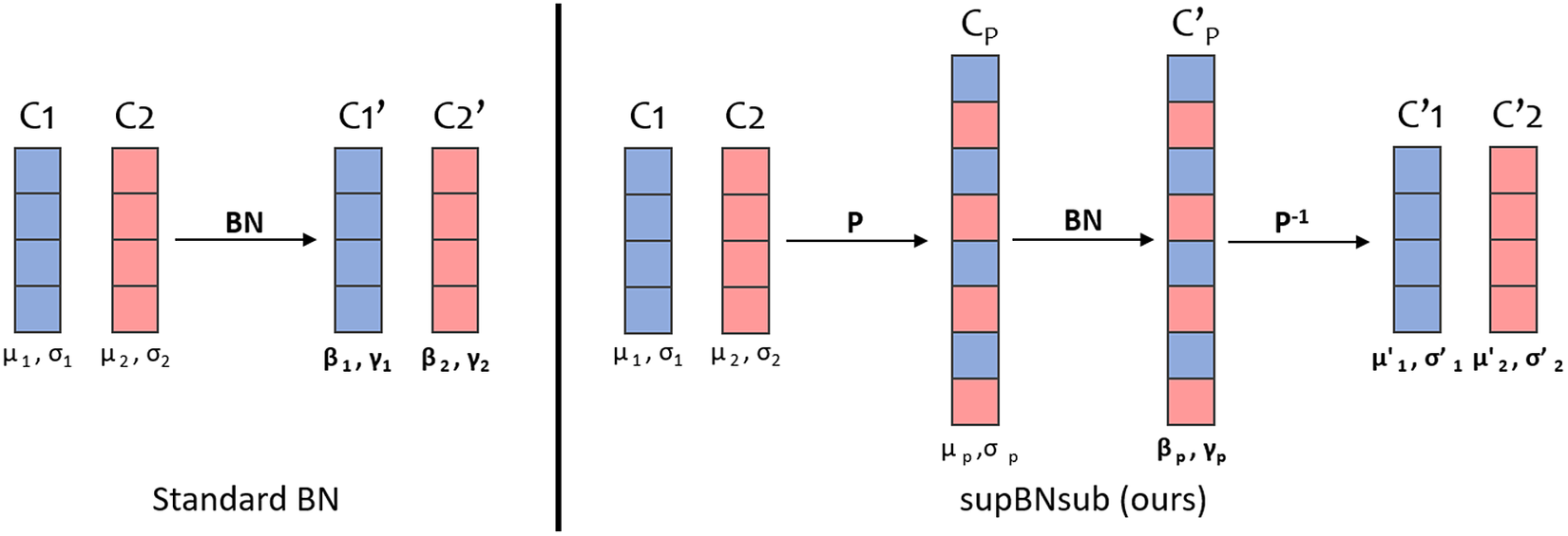
Figure 4. Comparison of the two BN methods for a one-dimensional example. For each channel, we write the mean and standard deviation below it and the learned parameters are in bold.
To explain why BN creates checkerboard artifacts, we must write the mean and standard deviation of both methods. It is trivial that in the case of the standard BN, the
 $ {C}_1^{\prime } $
channel has a mean of
$ {C}_1^{\prime } $
channel has a mean of
 $ {\beta}_1 $
and a standard deviation of
$ {\beta}_1 $
and a standard deviation of
 $ {\gamma}_1 $
(respectively,
$ {\gamma}_1 $
(respectively,
 $ {\beta}_2 $
and
$ {\beta}_2 $
and
 $ {\gamma}_2 $
for the
$ {\gamma}_2 $
for the
 $ {C}_2^{\prime } $
channel). According to notations in Figure 4, in the supBNsub case we have (see Appendix A for details)
$ {C}_2^{\prime } $
channel). According to notations in Figure 4, in the supBNsub case we have (see Appendix A for details)
 $$ {\mu}_p=\frac{\mu_1+{\mu}_2}{2}{\sigma}_p^2=\frac{\sigma_1^2+{\sigma}_2^2}{2}+{\left(\frac{\mu_1-{\mu}_2}{2}\right)}^2\hskip2em {\mu}_1^{\prime }={\gamma}_p\frac{\mu_1-{\mu}_p}{\sigma_p}+{\beta}_p{\sigma_1^{\prime}}^2=\frac{\gamma_p^2{\sigma}_1^2}{\sigma_p^2}. $$
In both cases, the output mean and standard deviation of the
 $ {C}_1^{\prime } $
and the
$ {C}_1^{\prime } $
and the
 $ {C}_2^{\prime } $
channels are not equal (Figure 4). During the upsampling operation to get back to the supspace, neighbors pixels will have slightly different values due to their different means, therefore some checkerboard artifacts will appear as shown in Figure 6. However, the supBNsub layer performs better than the standard BN because it has a higher regularization effect as all the channels are normalized the same way. The supBNsub layer has less degrees-of-freedom where the standard BN bias and standard deviation are completely unrelated between two different channels.
$ {C}_2^{\prime } $
channels are not equal (Figure 4). During the upsampling operation to get back to the supspace, neighbors pixels will have slightly different values due to their different means, therefore some checkerboard artifacts will appear as shown in Figure 6. However, the supBNsub layer performs better than the standard BN because it has a higher regularization effect as all the channels are normalized the same way. The supBNsub layer has less degrees-of-freedom where the standard BN bias and standard deviation are completely unrelated between two different channels.
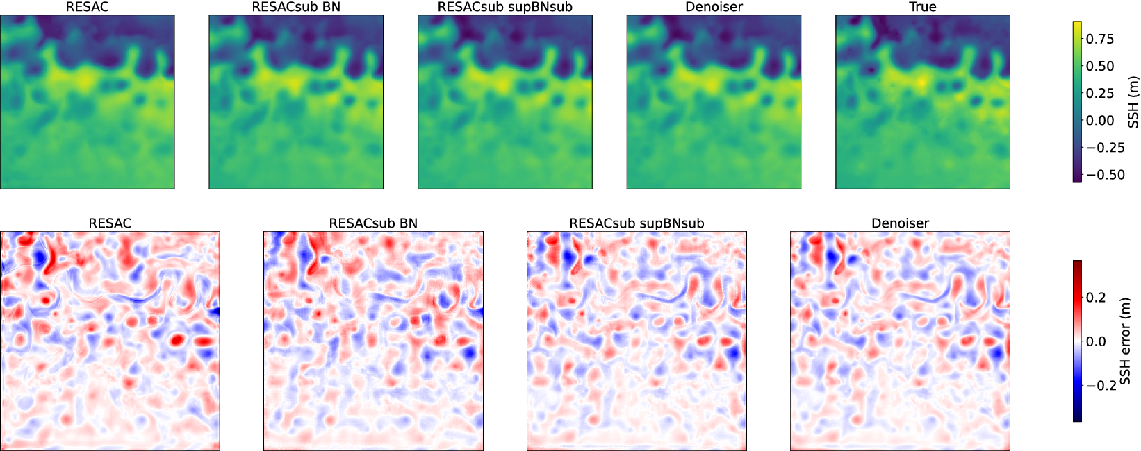
Figure 5. Network output for SSH at R03. The first line is the estimated SSH of the same day (March 10) and the second line is the error map associated.
Figure 6. Zoom on the error map of the two subpixel models RESACsub BN and RESACsub supBNsub, and the denoising network applied on RESACsub supBNsub. We can clearly see the
 $ 3\times 3 $
pattern on the two subpixel models, where the denoiser removes it.
$ 3\times 3 $
pattern on the two subpixel models, where the denoiser removes it.
The checkerboard artifacts are intrinsically linked to the subpixel convolutional layers, as different filter weights are applied to neighbor pixels. To get rid of this problem we use a post-trained denoising filter: at the end of RESACsub, we apply two convolution layers with 32 filters with a
 $ 7\times 7 $
kernel size and a ReLu activation function. This convolution operation is wide enough to perceive a
$ 7\times 7 $
kernel size and a ReLu activation function. This convolution operation is wide enough to perceive a
 $ 12\times 12 $
area where several checkerboard patterns should be repeated. After these two layers, we perform a last convolution layer with one filter
$ 12\times 12 $
area where several checkerboard patterns should be repeated. After these two layers, we perform a last convolution layer with one filter
 $ 1\times 1 $
and no activation to get back to the image dimension.
$ 1\times 1 $
and no activation to get back to the image dimension.
4. Results
We compare the results of four models on the validation data set. We call hereafter RESAC the network presented in Thiria et al. (Reference Thiria, Sorror, Mejia, Molines and Crepon2022), RESACsub supBNsub the proposed network with the supBNsub BN layer, RESACsub BN the same network but with the standard BN, and Denoiser stands for the denoising filter applied after the RESACsub supBNsub network. We also provide a bicubic interpolation as a baseline. For each upsampling architecture (a CNN block in Figure 1), both models have five loops (
 $ Nloop=5 $
), see Figure 2. For RESAC, that corresponds to 10 convolution layers with
$ Nloop=5 $
), see Figure 2. For RESAC, that corresponds to 10 convolution layers with
 $ 37 $
filters, and for RESACsub it corresponds to
$ 37 $
filters, and for RESACsub it corresponds to
 $ 10 $
convolution layers with
$ 10 $
convolution layers with
 $ 32 $
filters and
$ 32 $
filters and
 $ 5 $
with
$ 5 $
with
 $ 18 $
filters. We adjusted the number of filters in RESAC up to
$ 18 $
filters. We adjusted the number of filters in RESAC up to
 $ 37 $
so that the two models are comparable in terms of weight number. However, RESACsub is still around 5 times faster to compute. We train each network 10 times with different initialization, so the scores presented in Table 1 are the mean ± standard deviation on the different training. The RESAC, RESACsub supBNsub, and RESACsub BN networks are trained with a batch size of 32 and an adaptive learning rate. On the other hand, the Denoiser is trained with a batch of a single image. In Appendix C, we provide some implementation details and an ablation study of the BN layer.
$ 37 $
so that the two models are comparable in terms of weight number. However, RESACsub is still around 5 times faster to compute. We train each network 10 times with different initialization, so the scores presented in Table 1 are the mean ± standard deviation on the different training. The RESAC, RESACsub supBNsub, and RESACsub BN networks are trained with a batch size of 32 and an adaptive learning rate. On the other hand, the Denoiser is trained with a batch of a single image. In Appendix C, we provide some implementation details and an ablation study of the BN layer.
Table 1. Mean and standard deviation scores on 10 rounds of training of each architecture with different weight initializations.
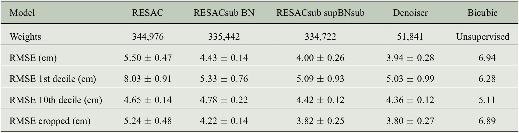
Note. The scores are given on the validation data set. We compare the models in RMSE (root mean squared error): the global RMSE is given, along with the RMSE on the first and the last decile of the target image. We also give a cropped RMSE (the RMSE of a smaller interior image to avoid border effects).
Table 2. Ablation study of the BN network.
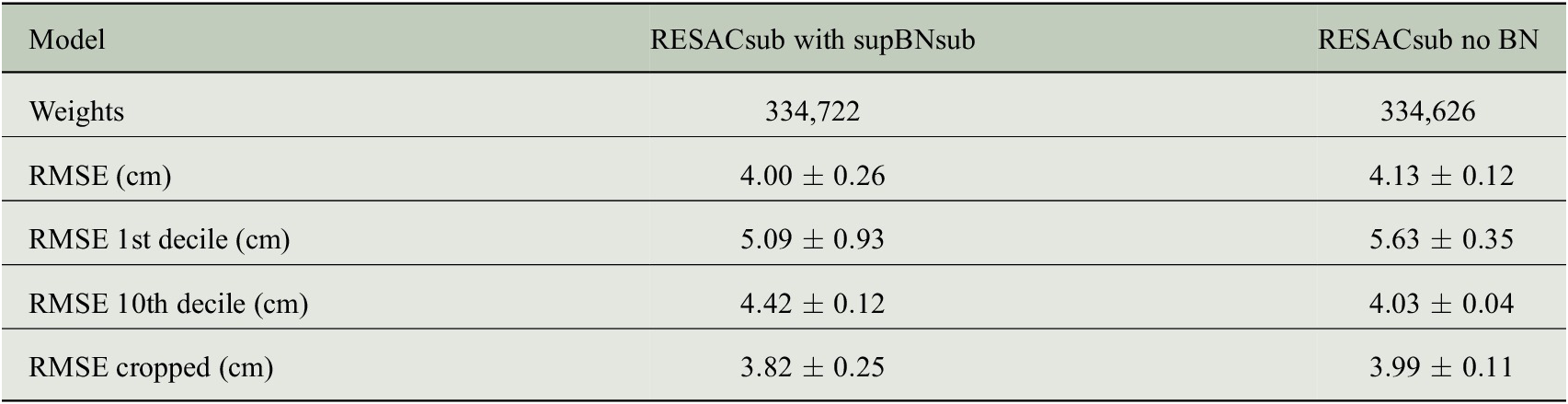
Note. Mean and standard deviation scores on 10 rounds of training of each architecture with different weight initializations.
The proposed model RESACsub with the supBNsup layer outperforms both RESAC and RESACsub with a standard BN. The denoising network improves the performances of RESACsub supBNsub on RMSE but also on the visual aspect by removing the checkerboard artifacts as shown in Figure 6.
On each image, we also identify the locations of the 10% highest and 10% lowest ground truth values and compute the RMSE of our downscaling at those locations (see Appendix B). As expected all the networks have a higher RMSE on the first decile (10% lowest values) than on the global image. This is because the North zone that has a low SSH is very energetic with very strong currents. Therefore the SSH variations are more important and less predictable. In Table 1, it is clear that most of the error is made in the north zone (corresponding to the lowest values).
5. Conclusion
We have proposed RESACsub, a subpixel convolutional residual network that outperforms RESAC in the Super Resolution task of downscaling SSH with high-resolution SST. Our method (RESACsub + denoising network) achieves a downscaling of 27 upsampling factor (from a resolution of
 $ 120\times 122\;{\mathrm{km}}^2 $
up to
$ 120\times 122\;{\mathrm{km}}^2 $
up to
 $ 4.5\times 4.5\;{\mathrm{km}}^2 $
) with an RMSE of 3.94 cm. We have compared two forms of BN: supBNsub, a subpixel adapted form of BN, and the standard BN. We show that the supBNsub method has higher regularizing power than the standard one which results in a performance improvement. However, the subpixel convolutional method has some drawbacks: it creates strong checkerboard artifacts on the output image. We were able to get rid of most of the checkerboard artifacts with a two layers-denoizing network that learns the
$ 4.5\times 4.5\;{\mathrm{km}}^2 $
) with an RMSE of 3.94 cm. We have compared two forms of BN: supBNsub, a subpixel adapted form of BN, and the standard BN. We show that the supBNsub method has higher regularizing power than the standard one which results in a performance improvement. However, the subpixel convolutional method has some drawbacks: it creates strong checkerboard artifacts on the output image. We were able to get rid of most of the checkerboard artifacts with a two layers-denoizing network that learns the
 $ 3\times 3 $
pattern and successfully denoises the SSH with a 0.06 cm RMSE improvement.
$ 3\times 3 $
pattern and successfully denoises the SSH with a 0.06 cm RMSE improvement.
To continue this work, we will push our approach further by not limiting it to a number of parameters similar to the ones in RESAC, which we suspect will yield even better results. This method could be declined to other bio-geophysical fields such as CHLA concentration if a learnable link exists between multiresolution data. We also intend to test and adapt our approach with other state-of-the-art architectures. Using the RESACsub network as a generator for a conditional generative adversarial neural (GAN) network similar to the SRGAN model introduced by Ledig et al. (Reference Ledig, Theis, Huszár, Caballero, Cunningham, Acosta, Aitken, Tejani, Totz and Wang2016) could improve its performance, given the advantages of using a discriminator network as a cost function for image reconstruction tasks. Further work also includes adapting this method to real-world satellite data using transfer learning to retain the skill obtained over the numerical model’s data set.
Acknowledgments
We are grateful for the technical assistance of Dr. M.Crépon.
Author Contributions
Conceptualization: T.A., A.C., D.B., S.T.; Data curation: C.M.; Data visualization: T.A.; Methodology: T.A., A.C.; Project administration: D.B., S.T.; Writing—original draft: T.A.; Writing—review & editing: T.A., A.C., D.B., S.T. All authors approved the final submitted draft.
Competing Interests
The authors declare no competing interests exist.
Data Availability Statement
The SARGAS60 data sets we used (extraction of the CJM155 and MJM155 NATL60 model experiments over the Gulf steam area, in the North Atlantic Ocean) are already available in the IPSL Thredds catalog at the address: https://doi.org/10.14768/c3c33afe-2a37-42e1-bb29-21428387f658.
Ethics Statement
The research meets all ethical guidelines, including adherence to the legal requirements of the study country.
Funding Statement
This research was supported by a grant for T. Archambault Ph.D. student from Sorbonne Université.
Provenance
This article is part of the Climate Informatics 2022 proceedings and was accepted in Environmental Data Science on the basis of the Climate Informatics peer review process.
A. Appendix: Proof of the Mean and Variance of the supBNsub Layer
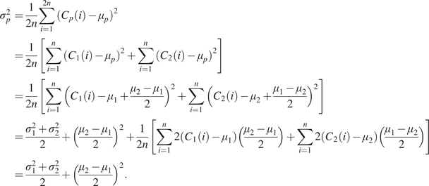 $$ {\displaystyle \begin{array}{ll}{\sigma}_p^2& =\frac{1}{2n}\sum \limits_{i=1}^{2n}{({C}_p(i)-{\mu}_p)}^2\\ {}& =\frac{1}{2n}\left[\sum \limits_{i=1}^n{({C}_1(i)-{\mu}_p)}^2+\sum \limits_{i=1}^n{({C}_2(i)-{\mu}_p)}^2\right]\\ {}& =\frac{1}{2n}\left[\sum \limits_{i=1}^n{\left({C}_1(i)-{\mu}_1+\frac{\mu_2-{\mu}_1}{2}\right)}^2+\sum \limits_{i=1}^n{\left({C}_2(i)-{\mu}_2+\frac{\mu_1-{\mu}_2}{2}\right)}^2\right]\\ {}& =\frac{\sigma_1^2+{\sigma}_2^2}{2}+{\left(\frac{\mu_2-{\mu}_1}{2}\right)}^2+\frac{1}{2n}\left[\sum \limits_{i=1}^n2\left({C}_1(i)-{\mu}_1\right)\left(\frac{\mu_2-{\mu}_1}{2}\right)+\sum \limits_{i=1}^n2\left({C}_2(i)-{\mu}_2\right)\left(\frac{\mu_1-{\mu}_2}{2}\right)\right]\\ {}& =\frac{\sigma_1^2+{\sigma}_2^2}{2}+{\left(\frac{\mu_2-{\mu}_1}{2}\right)}^2.\end{array}} $$
Because the BN do not changes the order of the pixels, we can see that
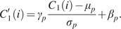 $$ {C}_1^{\prime }(i)={\gamma}_p\frac{C_1(i)-{\mu}_p}{\sigma_p}+{\beta}_p. $$
Then we can write
 $ {\mu}_1^{\prime } $
and
$ {\mu}_1^{\prime } $
and
 $ {\sigma}_1^{\prime } $
as
$ {\sigma}_1^{\prime } $
as
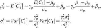 $$ {\displaystyle \begin{array}{l}{\mu}_1^{\prime }=E\left[{C}_1^{\prime}\right]={\gamma}_p\frac{E\left[{C}_1\right]-{\mu}_p}{\sigma_p}+{\beta}_p={\gamma}_p\frac{\mu_1-{\mu}_p}{\sigma_p}+{\beta}_p,\\ {}{\sigma}_1^{\prime }= Var\left[{C}_1^{\prime}\right]=\frac{\gamma_p^2}{\sigma_p^2} Var\left[{C}_1\right]=\frac{\gamma_p^2{\sigma}_1^2}{\sigma_p^2}.\end{array}} $$
B. Appendix: Metrics
In Table 1 we used several metrics that we detail hereafter.
 $$ \mathrm{RMSE}\left(\hat{y},y\right)=\sqrt{\frac{1}{n}\sum \limits_{\left(i,j\right)\in S}{\left({\hat{y}}_{ij}-{y}_{ij}\right)}^2}, $$
where
 $ \hat{y} $
and
$ \hat{y} $
and
 $ y $
are respectively the estimation and the truth at an instant,
$ y $
are respectively the estimation and the truth at an instant,
 $ S $
is the summation domain, and
$ S $
is the summation domain, and
 $ n $
is the cardinality of
$ n $
is the cardinality of
 $ S $
. All RMSEs of Table 1 are computed the same way but with various
$ S $
. All RMSEs of Table 1 are computed the same way but with various
 $ S $
. We consider
$ S $
. We consider
 $ y\in {\mathrm{IR}}^{HxH} $
, the summation domains are
$ y\in {\mathrm{IR}}^{HxH} $
, the summation domains are
-
• RMSE:
 $ S=\left\{\left(i,j\right)\hskip1em /\hskip1em 1\le i,j\le H\right\} $
,
$ S=\left\{\left(i,j\right)\hskip1em /\hskip1em 1\le i,j\le H\right\} $
, -
• RMSE cropped:
$ S=\left\{\left(i,j\right)\hskip1em /\hskip1em 6\le i,j\le H-6\right\} $
, -
• RMSE 1st decile:
$ S=\left\{\left(i,j\right)\hskip1em /\hskip1em {y}_{ij}\le {d}_1\right\} $
, where
$ {d}_1 $
is the first decile, -
• RMSE 10th decile:
$ S=\left\{\left(i,j\right)\hskip1em /\hskip1em {y}_{ij}\ge {d}_9\right\} $
, where
$ {d}_9 $
is the last decile.


C. Appendix: Implementation Details and Ablation Study
In this appendix, we give some implementation details.
-
• Optimizer: We use the ADAM optimizer with
$ {\beta}_1=0.9 $
,
$ {\beta}_2=0.999 $
and an initial learning rate of
$ 0.002 $
. -
• Learning Rate Scheduler: The learning rate scheduler is defined as follows. During the first 20 epochs, the learning rate stays constant, then from epoch 20 to epoch 60, the learning rate is multiplied at each epoch by
$ {e}^{-0.02} $
. Finally, after epoch 60 the learning rate is multiplied by
$ {e}^{-0.05} $
at each epoch until the end of the training. All the networks are trained during 150 epochs. -
• Weights Initialization Method: The weight initialization used for all convolutional layers is the “He normal” kernel initialization. The weights are taken from a truncated normal distribution centered on 0 with a standard deviation of
$ \hskip2.3em \sqrt{2/ in} $
where
$ in $
is the number of input units in the weight tensor. -
• BN Ablation Study: We performed an ablation study of the BN. After an extensive search of learning rate schedulers and of the number of epochs to train the network we found a combination that converged to similar results. We used a constant learning rate for 50 epochs and then multiplied it by
$ {e}^{-0.004} $
for each epoch. With no BN, the convergence is slower so we had to train the networks for 1,500 epochs: it is the main drawback of the lack of BN. RESACsub without BN is outperformed by the RESACsub supBNsub but the two models are close in terms of RMSE (see Table 2).


 Open access