


1. Introduction
Amid rising public awareness of environmental issues, eco-friendly technologies are gradually being adopted worldwide. Examples of such technologies include energy-efficient devices such as solar photo-voltaic cells, light-emitting diodes, and water-efficient washing machines and toilets. In this study, we focus on low-input turfgrass, a type of lawn grass that requires less water and fertilizer than conventional turfgrass and thus reduces environmental footprints. Sheffield and Wood (Reference Sheffield and Wood2008) predicted increasing global temperature will result in more droughts, and thus the environmental contribution of turfgrass that reduce water usage will become more crucial in the future. In addition, Gu et al. (Reference Gu, Crane, Hornberger and Carrico2015) examined the long-term impact of turfgrass management practice on global warming. They concluded that turfgrass acts as a net carbon emitter and recommended reduction of fertilization as the most effective carbon mitigation approach. Given the eco-friendly features of low-input turfgrass, this study investigates the factors that impact the adoption of this relatively new technology. Previous studies that examined household’s willingness to adopt eco-friendly technologies predominantly focused on the energy consumption. The adoption of turfgrass resembles energy-efficient technology adoption in the sense that consumers need to rationalize an upfront investment with delayed return under uncertainty. Despite eco-friendly technologies being seen as a “win-win” for adopters and the environment because the technologies can reduce both adopter expenditures and negative environmental impacts, the rate of adoption of such technologies has not been as high as expected (Greene et al., Reference Greene, German, Delucchi, Greene, German and Delucchi2009).
Previous studies of adoption of consumer technologies have primarily focused on two aspects: (1) evaluating the long-term benefit of adoption and (2) investigating consumers’ decision-making processes when considering adopting a new technology. Studies of the long-term benefits of adoption have predominantly addressed energy use and examined how much people benefit from technology adoption and whether there has been underinvestment in energy-saving technologies. For instance, Granade et al. (Reference Granade, Creyts, Derkach, Farese, Nyquist and Ostrowski2009) conducted a cost–benefit analysis of adopting an energy-efficient technology for end-users.Footnote 1 They concluded that the potential savings in terms of energy costs ($1.2 trillion) were much larger than the required investment ($520 million). Other studies compared energy use before and after adopting an energy-saving technology to evaluate potential cost savings. Schweitzer (Reference Schweitzer2005), for example, conducted a meta-analysis of studies of weatherization assistance programs and estimated that weatherization that cost about $2,600 could reduce natural gas use by 20%–25%, about $260 annually. However, Allcott and Greenstone (Reference Allcott and Greenstone2012) reviewed studies related to energy efficiency gaps, which refer to differences between actual and optimal levels of adoption of an energy-efficient technology. They argued that prior studies had underestimated the cost of technology adoption and, therefore, had overstated the magnitude of energy efficiency gaps.
Another body of literature has examined major factors affecting decisions about adoption of technology using behavioral economic frameworks. Technology adoption usually requires an upfront investment that only later generates returns, so understanding how households perceive the technology’s future value is crucial. Several studies examined consumer perceptions of future value using the exponential discounting framework. Busse, Knittel, and Zettelmeyer (Reference Busse, Knittel and Zettelmeyer2013) found that a $1 increase in the price of gasoline was associated with a significant increase in the market share and equilibrium price of highly fuel-efficient cars. Their estimates of implicit discount rates were low, suggesting that consumers were not myopic.
Other studies have estimated discounting factors using the exponential discounting framework and arrived at different conclusions. Allcott and Wozny (Reference Allcott and Wozny2014), for example, found that consumers equally valued a $1 discount in future gas costs and an immediate $0.76 discount in a vehicle purchase price. They concluded that vehicle consumers were significantly more myopic than financial market investors. Gillingham, Houde, and Van Benthem (Reference Gillingham, Houde and Van Benthem2019) found that consumers were indifferent between a $1 discounted future fuel cost and $0.15–$0.38 discounts in vehicle prices, resulting in a 4% discount rate. Their results suggest that consumers are even more myopic than identified by Allcott and Wozny (Reference Allcott and Wozny2014). Cohen, Glachant, and Söderberg (Reference Cohen, Glachant and Söderberg2017) also found that consumers in the United Kingdom heavily discounted future energy costs, estimating an implicit discount rate of 11%. De Groote and Verboven (Reference De Groote and Verboven2019) identified household discount factors using a program involving tradeoffs between a future household subsidy and an immediate upfront payment. They found that households heavily discounted future benefits from a new technology. For example, households were willing to pay approximately €0.5 upfront for every €1.0 of future benefit.
In addition to analyses using the exponential discounting framework, many studies have documented “present” bias in which individuals undervalue future gains or losses relative to present ones (Laibson, Reference Laibson1997; O’Donoghue and Rabin, Reference O’Donoghue and Rabin1999). Unlike exponential discounting, which analyzes discount values in two consecutive periods, models of present bias (e.g., hyperbolic discounting and quasi-hyperbolic discounting) predict how people further discount values in future periods relative to the discount value in the present period. Therefore, present bias models generalize the exponential discounting model.
Lastly, failure to adopt a new technology could be due to consumers’ uncertainty regarding its effectiveness and potential downsides. Several recent studies have emphasized the importance of including consumer uncertainty perception in analyses of new technology adoption (Greene, Reference Greene2011; Heutel, Reference Heutel2019; Schleich et al., Reference Schleich, Gassmann, Meissner and Faure2019). For instance, Greene (Reference Greene2011), using the expected utility framework, demonstrated that the investment required to increase car fuel economy from 28 to 35 miles per gallon should have a positive expected net present value (NPV) but also found that the investment was uninteresting to loss-averse consumers. These results potentially explain at least some underuse of energy-efficient technologies.
Tversky and Kahneman (Reference Tversky and Kahneman1992) found that individual perceptions of uncertainty do not follow the expected utility framework. Prospect theory (Kahneman and Tversky, Reference Kahneman and Tversky1979) proposes that individual perceptions of uncertainty consist of four elements: (1) reference dependence, (2) loss aversion, (3) diminishing sensitivity, and (4) probability weighting (Barberis, Reference Barberis2013). Thus, prospect theory enhanced expected utility specifications by adding several behavior parameters and is a generalization of the expected utility model. Barberis (Reference Barberis2013) reviewed developments in prospect theory and results of empirical studies and found that prospect theory characterizes individual uncertainty perceptions more accurately than the expected utility framework.
Our study builds on prior ones by analyzing behavior associated with adoption of a new technology by capturing consumers’ degree of risk aversion associated with present bias, weighting of probabilities, and aversion to loss using prospect theory in a choice experiment. This study is most related to Heutel (Reference Heutel2019) and Schleich et al. (Reference Schleich, Gassmann, Meissner and Faure2019) in the sense that it considers the effects of a comprehensive set of behavior parameters. Schleich et al. (Reference Schleich, Gassmann, Meissner and Faure2019) used multiple price lists with delayed returns to capture discount factors and present bias, lotteries to capture risk aversion and loss aversion, and a stated-decision survey to measure technology adoption preferences. They established a correlation between the behavioral parameters and stated decisions. Similarly, Heutel (Reference Heutel2019) conducted multiple experiments to capture participants’ behavior parameters and then analyzed correlation between those parameters and adoption of various types of energy-efficient technologies.
Our experimental design explicitly considers individuals’ tradeoffs between an upfront investment and its delayed benefits under uncertainty using a choice experiment, which is different from Heutel (Reference Heutel2019) and Schleich et al. (Reference Schleich, Gassmann, Meissner and Faure2019). The advantage of Heutel (Reference Heutel2019) and Schleich et al. (Reference Schleich, Gassmann, Meissner and Faure2019) approach is that price lists and lotteries can be incentivized to capture participants’ behavior parameters more accurately. However, their willingness to adopt technology is self-stated and thus hypothetical. In addition, these two studies intended to estimate the association between behavior parameters and consumers’ willingness to adopt new technology, while the role of upfront cost was not considered. The approach in this study aimed to capture the substitution patterns between upfront costs and uncertain future returns using a choice experiment.
In addition to capturing cost–benefit tradeoffs, choice experiment allows one to investigate the relative importance of various factors in shaping consumers’ technology adoption decisions. When making technology adoption decisions, consumers do not necessarily behave “rationally.” Besedeš et al. (Reference Besedeš, Deck, Sarangi and Shor2012), for example, showed that people use mental shortcuts (heuristics) to make complex decisions and that the heuristics shift their choices away from the “optimal rational decision.” Given that technology adoption is a complex decision that involves delayed benefit with uncertainty, participants may use mental shortcuts to simplify the complex decision. We explicitly explained to participants that the purpose of the seemingly complex choice experiment in this study is not to ask them to calculate the optimal decision; instead, we intend to characterize how consumers weigh the importance of factors with their decision heuristics. Furthermore, studies demonstrated that decision heuristics, for example, preference and risk perception, could vary by decision context (Siegrist and Árvai, Reference Siegrist and Árvai2020; Trueblood et al., Reference Trueblood, Brown, Heathcote and Busemeyer2013). Thus, choice experiment that simulates consumers’ turfgrass adoption with a clearly defined decision context is more appropriate.
The present study makes several valuable contributions. In terms of theory, we incorporate parameters associated with prospect theory (reference dependence, probability weighting, risk aversion, and diminishing sensitivity) and parameters that account for quasi-hyperbolic discounting (exponential discounting and present bias) into a choice experiment to identify how those factors affect decisions about adopting the technology. To our knowledge, our study is the first to apply such a comprehensive behavioral framework to capture household tradeoffs between the required investment and uncertain future returns in the context of technology adoption. Empirically, we develop a framework that can be easily adapted to other decisions that involve upfront investments and delayed returns under uncertainty. We also compare the results from our model to estimates from an expected utility specification with exponential discounting. We find that, as a generalization of the expected utility framework, the proposed model more accurately captures individuals’ intertemporal decisions under uncertainty. Lastly, our study of adoption of low-input turfgrass sheds light on households’ reasons for not adopting the technology and understanding the reasons that can improve adoption of it in the future. We present policy and marketing implications of our findings that apply to adoption of low-input turfgrass and to other new products and technologies. The objective of this study is not to prove our approach is better than the ones used in the previous studies because what model fits a data the best is often an empirical question. Rather, we propose an alternative comprehensive way to investigate people’s new technology adoption behavior and shed light on how marketing and policy could encourage new technology adoption.
2. Background
The choice experiment in our study presents participants with an opportunity to adopt turfgrass that require less water and fertilizer than traditional turfgrass. Hard fescue (Festuca brevipila Tracey), chewings fescue (Festuca rubra L. ssp. commutata Gaudin), and other similar fine fescues are alternatives to conventional species such as Kentucky bluegrass (Poa pratensis L.) and perennial ryegrass (Lolium perenne L.) for temperate climates commonly found in the northern United States, where lawns typically are an important part of urban landscapes and cover large areas (Milesi et al., Reference Milesi, Elvidge, Dietz, Tuttle, Nemani and Running2005). Kentucky bluegrass (Poa pratensis L.) is a winter-hardy turfgrass that requires relatively large amounts of water, fertilizer, and pesticides to meet consumers’ esthetic and functional requirements.
Public pressure to reduce the amount of water and chemicals required for lawns in the United States is increasing. Previous studies have examined the factors and interventions that may impact household water conservation behavior (Addo, Thoms, and Parsons, Reference Addo, Thoms and Parsons2018; Fielding et al., Reference Fielding, Russell, Spinks and Mankad2012; Goette, Leong, and Qian, Reference Goette, Leong and Qian2019; Qaiser et al., Reference Qaiser, Ahmad, Johnson and Batista2011; Willis et al., Reference Willis, Stewart, Panuwatwanich, Williams and Hollingsworth2011). Many states, including Minnesota, have recently imposed restrictions on phosphorus fertilizer (Lee and McCann, Reference Lee and McCann2018), and outdoor watering restrictions are common throughout the country (Milman and Polsky, Reference Milman and Polsky2016). As concern about droughts associated with climate change (Sheffield and Wood, Reference Sheffield and Wood2008) intensifies, pressure to reduce water dedicated to home lawns will likewise increase. Previous studies have established that social awareness and exposure to drought affect residents’ attitudes toward water saving (Beal, Stewart, and Fielding, Reference Beal, Stewart and Fielding2013; Knuth et al., Reference Knuth, Behe, Hall, Huddleston and Fernandez2018). Knuth et al. (Reference Knuth, Behe, Huddleston, Hall, Fernandez and Khachatryan2020) showed that plant watering requirement plays a more important role for residents of states who frequently experienced drought.
Reducing inputs required for lawns can be accomplished using various approaches, but perhaps the most effective is using alternative turfgrass species. Previous studies have demonstrated that low-input turfgrass can perform well with limited water and no fertilizer or pesticides and require less mowing (Diesburg et al., Reference Diesburg, Christians, Moore, Branham, Danneberger, Reicher, Voigt, Minner and Newman1997; Hugie and Watkins, Reference Hugie and Watkins2016; Watkins et al., Reference Watkins, Fei, Gardner, Stier, Bughrara, Li, Bigelow, Schleicher, Horgan and Diesburg2011). Several studies have shown that consumers are willing to pay premium prices for certain attributes of low-input turfgrass. Yue, Hugie, and Watkins (Reference Yue, Hugie and Watkins2012) conducted a choice experiment targeting Minnesota consumers and found that they are willing to pay premiums for turfgrass that requires less irrigation, fertilization, and mowing. Similarly, Yue et al. (Reference Yue, Wang, Watkins, Bonos, Nelson, Murphy, Meyer and Horgan2017) found that consumers in the United States and Canada are willing to pay a statistically significant price premium for turfgrass that leads to less watering, fertilizer inputs, and mowing. Hugie, Yue, and Watkins (Reference Hugie, Yue and Watkins2012) conducted a conjoint analysis and found that maintenance attributes in general and irrigation requirements in particular have significant effects on consumers’ willingness to purchase low-input turfgrass seeds. Ghimire et al. (Reference Ghimire, Boyer, Chung and Moss2016) found that consumers in the southern United States rank low maintenance, drought tolerance, and saline tolerance as the most desirable lawn attributes.
Despite the numerous benefits of low-input turfgrass and evidence that consumers are willing to pay a premium for those benefits, adoption of low-input turfgrass for lawns in the United States has been limited (Braun et al., Reference Braun, Patton, Watkins, Koch, Anderson, Bonos and Brilman2020). All of the previously mentioned studies assumed that the alternative turfgrasses would perform as well as conventional ones and did not consider potential adoption risks. As with any new product, adoption of a new turfgrass involves uncertainty about its performance. Low-input turfgrass could be susceptible to diseases and/or weeds that would not be problematic for conventional species, for example, and consumers likely would know less about the new species’ specific management requirements. Our study investigates consumer decision-making about low-input turfgrass from a behavioral perspective to shed light on factors that prevent consumers from adopting this useful technology.
3. Experiment Design
To investigate barriers to adoption of low-input turfgrass, we first convened a focus groupFootnote 2 involving a small number of homeowners. We asked them about their turfgrass maintenance practices, the attributes of the grasses that were most important to them, and their awareness of alternative turfgrass requiring fewer inputs. We also showed participants a sample square of sod planted with a low-input turfgrass and asked them about their preferences regarding the grass and their willingness to switch to it. We found both limited adoption of the low-input turfgrass and little awareness of such grasses as an alternative for lawns. The focus group discussion revealed several prevalent concerns that potentially prevent participants from adopting low-input turfgrass: the amount of effort required to replace the entire lawn at once, uncertainty about whether the new turfgrass would survive, and whether the long-term cost and time savings would cover the initial investment cost.
We used the results of the focus group to design our choice experiment analyzing homeowners’ decisions regarding adoption of low-input turfgrass. Specifically, since the effort required to completely convert a lawn to low-input turfgrass was a concern, we included three options in the choice experiment: one option replaced all of the conventional grass at once using sod and two options replaced the conventional grass gradually using overseeding. Note that the one-time full replacement option provides an immediate return on the investment while the gradual replacement options provide delayed returns. To address expressed concerns about the alternative turfgrass failing to survive, we included the probability of success for the low-input turfgrass and the additional expense required to replace it if it failed. We assumed that participants’ reference points were to the status quo of conventional turfgrass and that all of their calculations of time saved, costs incurred, and potential gains would be based on their current investments in their lawns.
In the choice experiment, participants were first given an introduction to low-input turfgrass:
Low input turfgrasses are those that can provide a functional, aesthetically pleasing lawn while not needing as much maintenance (less watering, less fertilizing, fewer pesticide applications, and less mowing) as more traditional turfgrasses like Kentucky bluegrass. These low-input turfgrasses are often characterized by a combination of low-input traits such as slow vertical growth, resistance to insects and diseases, tolerance of drought, and ability to maintain quality without a lot of fertilization.
The experiment administrators then explained the context of the choice experiment, which presented participants with scenarios simulating a situation in which a lawn service company provided a service converting conventional lawn grasses to low-input turfgrasses. The lawn service setting was designed to eliminate potential confusion among participants regarding the amount of effort required to make the switch. Participants then received a detailed written explanation of the choice scenarios. In each choice task, participants would be presented with three replacement options (one full replacement and two gradual replacements), and the instruction stressed that there was no “correct answer” and that their task was to determine which option provided them with the greatest overall value and worked best for their households.
Each choice scenario consisted of four options—the three replacement options (A, B, and C) and the option to opt-out and decline conversion (D). Option A represented full immediate replacement using sod and delivered returns immediately since there was no need to wait for seeds to germinate and become established. This option not only represents the most rapid way to adopt the technology but also involves the greatest upfront investment of time and money. Option B represented conversion over an intermediate length of time of 2 years using overseeding. During those two transitional years, there was a cost per year for seed and participants would begin to obtain the benefit of conversion at the beginning of the third year. Option C represented a slower overseeding conversion of 3 years, a fixed investment cost for seed, and benefits obtained at the beginning of the fourth year. As defined by prospect theory, the losses and gains from conversion and their associated probabilities are relative to the status quo, which is the participant’s current lawn, and Option D is the status quo.
Each option presented in the experiment was characterized by five attributes. The first was the upfront cost (sod, seed) per 1,000 ft2, which was $600, $800, and $1000 under Option A; $300, $400, and $500 under Option B; and $240, $320, and $400 under Option C. The second attribute was time savings of 20%, 40%, and 60% provided by low-input turfgrass during the growing season (less mowing, watering, and fertilizing). The third attribute was potential cost saved per year after completing the conversion, thanks to reduced needs for water and fertilizer, which was set at $200, $250, and $300. The fourth attribute was probability of success of the new turfgrass (that it would grow as expected and require no further investment), which was set at 70%, 80%, and 90%. The fifth attribute was the additional investment required if the alternative product failed; it was set at $150, $175, and $200.Footnote 3 We designed the choice experiment with optimal D-efficiency.
The choice experiment was designed to capture intertemporal discounting, present bias, probability weighting, risk aversion, and loss aversion. To capture present bias, we asked participants to choose between immediate adoption with a high one-time investment cost and slower adoption with a lower per-period investment cost over multiple periods. Gradual adoption under Options B and C, which have different transition periods, was designed to capture the discounting factor. The varying probabilities of gains and losses were designed to capture probability weighting, and the varying amounts of losses and gains were designed to capture loss aversion and risk aversion.
We conducted the experiment in 2019 and used Qualtrics™, a professional survey company, to obtain a representative sample of U.S. homeowners 18 years of age or older. Interested participants were first asked a screening question: “Do you have a home lawn?” Individuals who answered yes were allowed to participate in the data-collection survey conducted prior to the choice experiment. Since the experiment design involved a 3-year transition period under Option C, the survey asked participants whether they expected to live at their current residences for less than 3 years and excluded all participants who answered affirmatively. The final sample for the choice experiment consisted of 866 participants.
4. Model Setup and Estimation Strategy
To analyze the results from the choice experiment, we set up a model that incorporates both prospect theory and intertemporal choice with present bias to capture how homeowners make decisions about adopting low-input turfgrasses. Let i = {1, …, I} denote homeowner i; j = {0, 1, 2, 3} denote opt-out Option D, Option A, Option B, and Option C, respectively, and ν ij the utility function of individual i choosing option j with opt-out utility normalized to 0 (ν i0 = 0). Assuming that the value function of the options, u ij , has the separable additive form,
 $${{u_{ij}} = {{\rm{\nu }}_{ij}} + {\varepsilon _{ij}}}$$
where u ij is the value function from option j and ϵ ij is the random utility error term assumed to be type-I extreme-value distributed. Thus, by McFadden (Reference McFadden1974), the probability of individual i choosing option j can be defined as
 $${{s_{ij}} = P{r_i}\left( {{u_{ij}} \ge \mathop {\max }\limits_{k \in \left\{ {0,1,2,3} \right\}} \{ {u_{ik}}\} } \right) = {{exp\left( {{\nu _{ij}}} \right)} \over {1 + \mathop \sum \nolimits_{k = 1}^3 exp\left( {{{\rm{\nu }}_{ik}}} \right)}}}.$$
Individual i evaluates the utility from option j at a finite horizon that is assumed to be the expected duration of individual i’s residency at the current location. Let T 1 denote the length of the transition period, which is one of the predefined attributes, and T 2 denote the expected duration of residence. We directly asked participants how long they expected to live at their current addresses. The utility from option j should consist of three components: (1) utility from average time savings per period (&#xi; j ), (2) the net present monetary value of the investment (η j ), and (3) the alternative-specific constant term (a i ). Assuming utility takes the separable additive form,
 $${{{\rm{\nu }}_{ij}} = {{\rm{a}}_j} + {{\rm{\omega }}_2}{{\rm{\xi }}_j} + {{\rm{\omega }}_1}{{\rm{\eta }}_j}}.$$
In equation (3), ω1 and ω2 are the marginal utility from average time savings and the net present monetary value of the investment, respectively.
When assuming exponential discounting, expected utility ν ij should take the form
 $$\eqalign{ {\nu _{ij}} = \,& {a_j} + {{\rm{\omega }}_2}\mathop \sum \nolimits_{t = {T_1} + 1}^{{T_2}} {{\rm{\beta }}_2}^t{{\rm{\tau }}^{{{\rm{\gamma }}_2}}}/\left( {{T_2} - {T_1}} \right) \cr & \!+ {{\rm{\omega }}_1}\left\{ \mathop \sum \nolimits_{t = {T_1} + 1}^{{T_2}} {{\rm{\beta }}_1}^t\left[ {{\rm{\pi }}{g^{{{\rm{\gamma }}_1}}} - \left( {1 - {\rm{\pi }}} \right){l^{{{\rm{\gamma }}_1}}}} \right] - \mathop \sum \nolimits_{t = 0}^{{T_1}} {{\rm{\beta }}_1}^t{c^{{{\rm{\gamma }}_1}}}\right\}. \cr} $$
In equation (4), β is the exponential discounting factor, τ is the time savings per period relative to current practice (percentage), γ
1 and γ
2 are the risk-aversion parameters, π is the probability of gain, and c
t
, g
t
, and l
t
are the cost, potential gain, and potential loss in period t, respectively. The average present value of time saving is
 $\xi _{j}=\sum _{t=T_{1}+1}^{T_{2}}{\beta _{2}}^{t}\tau ^{{\gamma _{2}}}/(T_{2}-T_{1}),$
the expected total present value due to loss and gain generated by low-input turfgrass is
$\xi _{j}=\sum _{t=T_{1}+1}^{T_{2}}{\beta _{2}}^{t}\tau ^{{\gamma _{2}}}/(T_{2}-T_{1}),$
the expected total present value due to loss and gain generated by low-input turfgrass is
 $\sum _{t=T_{1}+1}^{T_{2}}{\beta _{1}}^{t}[\pi g^{{\gamma _{1}}}-(1-\pi )l^{{\gamma _{1}}}],$
and the present value of the total cost is
$\sum _{t=T_{1}+1}^{T_{2}}{\beta _{1}}^{t}[\pi g^{{\gamma _{1}}}-(1-\pi )l^{{\gamma _{1}}}],$
and the present value of the total cost is
 $\sum _{t=0}^{T_{1}}\beta ^{t}c^{{\gamma _{1}}}.$
Thus,
$\sum _{t=0}^{T_{1}}\beta ^{t}c^{{\gamma _{1}}}.$
Thus,
 $$\eta _{j}=\sum _{t=T_{1}+1}^{T_{2}}\beta ^{t}[\pi g^{{\gamma _{1}}}-(1-\pi )l^{{\gamma _{1}}}]-\sum _{t=0}^{T_{1}}\beta ^{t}c^{{\gamma _{1}}}.$$
To account for present bias, loss aversion, and probability weighting, the model takes the form
 $$\eqalign{ {\nu _{ij}} = & \, {a_j} + {{\rm{\omega }}_2}\mathop \sum \nolimits_{t = {T_1} + 1}^{{T_2}} {\beta _2}^t{{\rm{\tau }}^{{\gamma _2}}}/\left( {{T_2} - {T_1}} \right) \cr & \!+ {{\rm{\omega }}_1}\left\{ \mathop \sum \nolimits_{t = {T_1} + 1}^{{T_2}} \alpha {\beta _1}^t\left[ {w\left( \pi \right){g^{{\gamma _1}}} - w\left( {1 - \pi } \right)\lambda {l^{{\gamma _1}}}} \right] - \mathop \sum \nolimits_{t = 0}^{{T_1}} {\alpha ^{{1_{t \gt 0}}}}{\beta _1}^t\lambda {c^{{\gamma _1}}}\right\}. \cr} $$
The difference between equations (4) and (5) is three components: the quasi-hyperbolic discounting (Laibson, Reference Laibson1997) parameter α used to capture present bias, the probability weighting function w(⋅), and the loss-aversion parameter λ. The functional form suggested by prospect theory is adapted from Tversky and Kahneman (Reference Tversky and Kahneman1992) with the individual evaluating losses and gains according to the function
 ${V}(\cdot )$
,
${V}(\cdot )$
,
 $${V\left( {\rm{x}} \right) = \left\{ {\matrix{ {{x^{{{\rm{\gamma }}_1}}}} & {if\;x \ge 0} \cr { - {\rm{\lambda }}{{\left( { - x} \right)}^{{\gamma _1}}}} & {if\;x \lt 0} \cr } } \right.,}$$
and the probability weighting function,
 $${w\left( {\rm{\pi }} \right) = {{{{\rm{\pi }}^{\rm{\mu }}}} \over {{{\left( {{{\rm{\pi }}^{\rm{\mu }}} + {{\left( {1 - {\rm{\pi }}} \right)}^{\rm{\mu }}}} \right)}^{1/{\rm{\mu }}}}}}.}$$
It is straightforward to see that equation (5) is a generalization of equation (4); that is, equation (5) becomes equation (4) when α = 1, μ = 1, and λ = 1. We assume an individual’s reference point is the status quo.
Having specified an individual’s utility and likelihood, we estimate the distribution of the parameters using Bayesian inference. The choices made by the participants are represented by
 ${Y}=\{y_{1},\ldots,y_{I}\}$
, a vector in which each element represents one of the four options in a choice scenario (opt-out, A, B, and C). We are interested in estimating the cumulative distribution function of the parameters (e.g., F(Θ|Y)). However, the nonlinear nature of the value function makes it difficult to solve using optimization algorithms so we use Bayesian inference instead. We assume that the prior cumulative distribution of the parameters was
${Y}=\{y_{1},\ldots,y_{I}\}$
, a vector in which each element represents one of the four options in a choice scenario (opt-out, A, B, and C). We are interested in estimating the cumulative distribution function of the parameters (e.g., F(Θ|Y)). However, the nonlinear nature of the value function makes it difficult to solve using optimization algorithms so we use Bayesian inference instead. We assume that the prior cumulative distribution of the parameters was
 $$\left\{ {\quad \matrix{ {{\beta _1} \sim U\left( {0,1} \right)} \hfill \cr {{\beta _2} \sim U\left( {0,1} \right)} \hfill \cr {\alpha \sim U\left( {0,1} \right)} \hfill \cr {\mu \sim N\left( {1,1} \right)} \hfill \cr {\lambda \sim N\left( {3,2} \right)} \hfill \cr {{\gamma _1} \sim U\left( {0,1} \right)} \hfill \cr {{\gamma _2} \sim U\left( {0,1} \right)} \hfill \cr {{\tau _1} \sim N\left( {0,3} \right)} \hfill \cr {{\tau _2} \sim N\left( {0,3} \right)} \hfill \cr {{a_j} \sim N\left( {0,3} \right)} \hfill \cr } } \right.$$
where U(⋅,⋅) refers to a uniform distribution and N(⋅,⋅) denotes a normal distribution. By Bayes’ theorem, the distribution of the parameters is proportional to
 ${F}({Y}|\Theta ){F}(\Theta )$
. In other words,
${F}({Y}|\Theta ){F}(\Theta )$
. In other words,
 $${F\left( {{\rm{\Theta |}}Y} \right) \propto F\left( {{\rm{Y|\Theta }}} \right)F\left( {\rm{\Theta }} \right)}$$
where F(Y|Θ) is the likelihood function and F(Θ) is the distribution of the parameters. The likelihood function F(Y|Θ) is given by
 $${F\left( {Y{\rm{|\Theta }}} \right) = \mathop \prod \limits_{i \in \left\{ {1,..,I} \right\}} \mathop \prod \limits_{j \in \left\{ {0,1,2,3} \right\}} s_{ij}^{{1_{\left\{ {{y_i} = j} \right\}}}}{{\left( {1 - {s_{ij}}} \right)}^{{1_{\left\{ {{y_i} \ne j} \right\}}}}}.}$$
The prior probability function is given by equation (8).
The posterior distribution F(Θ|Y) is estimated using a differential-evolution Markov chain Monte Carlo (MCMC) method (ter Braak and Vrugt, Reference ter Braak and Vrugt2008) and implemented using BayesianTools in R (Hartig et al., Reference Hartig, Minunno, Paul, Cameron, Ott and Pichler2019). We employed seven chains in the MCMC process, which allowed for testing of convergence. We ran each chain until the last 5,000 iterations indicated convergence. That is, until the potential scale reduction factor (PSRF) was less than 1.1 for all parameters, the convergence threshold suggested by Brooks and Gelman (Reference Brooks and Gelman1998).
5. Results
Table 1 presents summary socio-demographic statistics for the 866 participants in the choice experiment. More than half expected to live in their current residences for at least an additional 15 years. Note that we use this information for the variable T 2 in equations (4) and (5). Participants’ yard sizes varied from less than 1/8 acre to more than 1 acre. We also collected the information on how much time participants spent on lawn maintenance. Our survey shows that most participants reported maintaining their lawns weekly or biweekly during growing seasons, and they spent 30 minutes to 2.5 hours each time. The median age of the participants fell in the 56–65 category and about 45% had a college degree. Most of the households (70%) were occupied by less than four people and 74% had annual household incomes of no more than $80,000. The choice probabilities of each option by scenarios are presented in Table A2 in the Appendix.
Table 1. Summary statistics of participants’ socio-demographic characteristics

Notes: Participants answered “not applicable” for frequency, time, and cost on lawn maintained were those who hired lawn services. Our survey asked if participants maintained their lawn on their own, and those who answered “yes” were directed to answer the questions related to their maintenance practices.
We used the last 4,000 iterations of each Markov chain to determine the density of the parameters. We first estimated the expected utility model with constant exponential discounting, which corresponds to equation (4). Table 2 summarizes the estimation results for each parameter, including the PSRFs, maximum a posteriori (MAP)Footnote 4 , 2.5 percentiles, medians, and 97.5 percentiles. Figure 1 presents the distribution of the parameters. All coefficients have PSRF values less than the 1.1 convergence threshold, and we further demonstrate convergence by presenting trace plots of each iteration from the seven Markov chains in Figure A1 in the Appendix. Each trace plot connects the values of the iterations and the line represents regression of the value of the coefficient against the nth iteration. This visual representation also indicates that the last 4,000 iterations reached a steady state.

Figure 1. Distribution of parameters, traditional exponential discounting model.
Table 2. Coefficient summary statistics, exponential discounting model
The most noticeable result from the expected utility model is the MAP-estimated discounting factor of 0.761. Figure 2 presents the estimated discounting level over 15 years. In the figure, the y-axis represents the cumulative discounting factor, β1 t , and the x-axis represents the tth year. The exponential curve plots the discounting level over time estimated using the exponential discounting model. Figure 2 shows that monetary benefits that will occur five or more years later are discounted by more than 75%. Therefore, based on this MAP estimator, a primary barrier to adoption of a new technology is intertemporal time discounting.

Figure 2. Effect of intertemporal time discounting.
To account for the other important factors identified in the focus group, we then extended the expected utility model to incorporate behavioral factors. We adapted the prospect theory model to evaluate present bias by including a quasi-hyperbolic discounting factor α, a probability weighting function
 ${w}(\cdot )$
, and a loss-aversion parameter λ as in equation (5). Figure 3 presents the corresponding density functions, and Table 2 presents summary statistics for the parameter distributions.
${w}(\cdot )$
, and a loss-aversion parameter λ as in equation (5). Figure 3 presents the corresponding density functions, and Table 2 presents summary statistics for the parameter distributions.

Figure 3. Distribution of parameters, behavioral model.
Let M
B
and M
E
denote the behavior model and expected utility model, respectively. We use the Bayes factor,
 ${Pr\left(Y|M_{B}\right) \over Pr\left(Y|M_{E}\right)}$
, to compare model goodness-of-fit. The log of the Bayes factor is 49.05, which results in a Bayes factor much larger than 100; this indicates that the behavioral economic model fits the data much better than the expected utility model with exponential discounting. As Table 3 indicates, the PSRFs are all less than the 1.1 convergence threshold (see also trace plots in Figures A2 and A3 in the Appendix).
${Pr\left(Y|M_{B}\right) \over Pr\left(Y|M_{E}\right)}$
, to compare model goodness-of-fit. The log of the Bayes factor is 49.05, which results in a Bayes factor much larger than 100; this indicates that the behavioral economic model fits the data much better than the expected utility model with exponential discounting. As Table 3 indicates, the PSRFs are all less than the 1.1 convergence threshold (see also trace plots in Figures A2 and A3 in the Appendix).
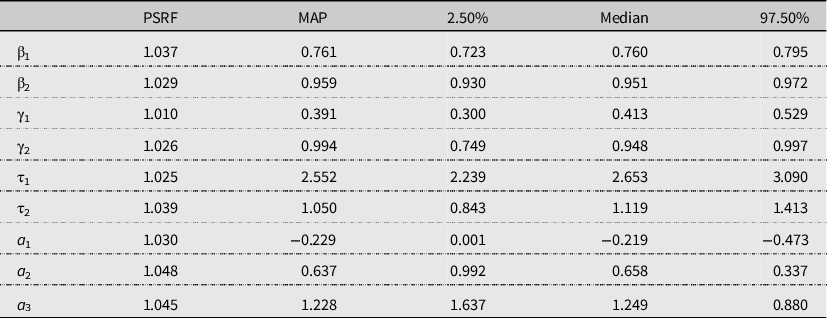
Table 3. Coefficient summary statistics, behavioral model

The results from the behavioral economic model are somewhat different from the ones from the expected utility model. First, we find that participants exhibit strong present bias; the quasi-hyperbolic discounting factor α has a MAP of 0.73 so all future values are discounted by 73% relative to present values. In addition to present bias, we find virtually no long-term discounting over time. Participants’ exponential discounting factors, β1 and β2, are very close to 1. Figure 2 presents the level of discounting estimated using the behavioral model. After a 73% discount in year 1, discounting remains virtually unchanged thereafter. Therefore, we find, based on the behavioral model, that consumers tend to heavily discount future values (a 73% discount rate) but that long-term benefits still play a significant role in their decisions. For example, consider a simplified case in which, at current period t = 0, the technology requires a $1,000 upfront investment and potential returns of $200 per period over 15 periods. In this case, the investment, when considering only the upfront cost, total benefit over time, and discounting factor, would be unprofitable based on estimates from exponential discounting. The NPV would be $826.23 – $1,000.00 = –$173.77. However, when using the behavioral model, the NPV is $2,327.02 – $1,000.00 = $1,327.02, making it an attractive investment.
Additionally, the behavioral model suggests that loss aversion is likely to be the primary barrier to adoption of low-input turfgrass rather than heavy discounting of future benefits. As the MAP of λ indicates, the absolute loss is valued almost six times more than the gain, suggesting that a warranty that would prevent losses should the new turfgrass fail to grow could be an effective way to promote adoption. Table 4 shows the results of simulating the impact of a warranty based on the ten choice scenarios, presenting observed probabilities of choosing to opt out and the simulated opt-out probability when a warranty covers potential losses. We find that provision of a warranty prominently boosted the likelihood that consumers would choose some form of lawn conversion rather than opting out.
Table 4. Simulated effect of warranty

Notes: Scenario refers to the choice experiment scenarios in which participants were asked to make choices about switching to low-input turfgrass.
Currently, the market does not offer service plans that assist homeowners in gradually switching to low-input turfgrasses. We simulated the market response to a program that resulted in time savings of 30% relative to current practices and required a one-time upfront cost of $1,000 to replace the existing lawn. We also simulated potential gains and losses relative to current practice ranging from $0 to $500.
We conducted a robustness check of the claim that (1) consumers are moderately myopic in the sense that they exhibit present bias that discounts all future values but the exponential discounting values are small and (2) consumers show strong loss aversion by deriving estimates of the same parameters (PSRF, MAP, 2.5 percentile, median, and 97.5 percentile) for sub-samples of participants. The sub-samples were based on age (younger than 65, 65 or older), education (a college degree, no college degree), income ($50,000 or less, more than $50,000), and gender (male, female). The results are shown in Table A1 in the Appendix.
The results in Appendix Table A1 support the robustness of the behavioral model with the full sample. We find that the exponential discounting factor is very close to 1 for all subgroups and that future value discounting is generated primarily by present bias. The robustness check shows, for example, that male participants, participants who had obtained a college degree, and participants whose incomes exceeded $50,000 discounted all future values by 60%–65% relative to present values. The present bias discounts for the other subgroups were smaller. The robustness check further supports the results for the whole sample in terms of loss aversion as the parameters are greater than 4 for all subgroups.
We further analyzed how homeowners valued time saved on maintenance with low-input turfgrasses, which require less mowing. We measured the monetary value of time savings using willingness to pay (WTP), which reflects a homeowner’s tradeoff between a one unit of (discounted) average maintenance time saving and a one unit of monetary cost. The monetary cost would be constant under linear utility. However, because of the nonlinearity of utility in our model, WTP in this case is a nonlinear function of time savings and cost:
 $${{{\partial {v_{ij}}/\partial {\rm{\tau }}} \over {\partial {v_{ij}}/\partial c}} = {{{{\rm{\omega }}_2}{{\rm{\gamma }}_2}\mathop \sum \nolimits_{t = {T_1} + 1}^{{T_2}} \alpha {\beta _2}^t{{\rm{\tau }}^{{{\rm{\gamma }}_2} - 1}}/\left( {{T_2} - {T_1}} \right)} \over {{{\rm{\omega }}_1}{{\rm{\gamma }}_1}\mathop \sum \nolimits_{t = 0}^{{T_1}} {\alpha ^{{1_{t \gt 0}}}}{\beta _1}^t\lambda {c^{{{\rm{\gamma }}_1} - 1}}}}.}$$
Figure 4 plots participants’ WTP for time savings for different levels of investment and average time savings for the scenarios in which they made one-time upfront investments and completely converted their lawns to low-input turfgrass. Because of decreasing marginal sensitivity, additional WTP to further decrease maintenance time increases the percent maintenance time savings. The simulated WTP values range from $3.50 to $4.10 for a 1% increase in time savings.

Figure 4. Simulated willingness to pay for time savings, one-time investment rapid adoption.
The probability weighting parameter μ has a MAP of 0.830. In Figure 5, the bold red line plots the estimated probability weighting function and the 45-degree line represents μ = 1. The figure shows that homeowners’ subjective perceptions of probability diverge only slightly from the 45-degree line.

Figure 5. Probability weighting function.
6. Discussion and Conclusions
Technologies such as fuel-efficient cars, solar photo-voltaic panels, and low-input turfgrasses for lawns are cost-effective ways to improve the health of consumers and the environment. Despite their many benefits, however, many of these technologies have failed to take hold in the market with actual adoption rates far below the economically efficient level (Greene et al., Reference Greene, German, Delucchi, Greene, German and Delucchi2009). Technology adoption typically requires an upfront expense in exchange for long-term future returns, so it is crucial to understand how consumers weigh such intertemporal costs and benefits. Additionally, new technologies, by definition, are not yet proven and can fail to deliver the expected benefits. And, as outlined in the introduction, numerous studies have shown that consumers do not necessarily behave according to predictions by expected utility frameworks. Consequently, to promote adoption of environmentally friendly technologies, we must consider alternative models such as prospect theory. We designed a choice experiment that simulated consumer decision-making and explicitly accounted for tradeoffs between an upfront investment cost and potential future gains and losses under uncertainty and present bias.
The empirical results of this study lead to two important conclusions. First, though households’ decisions are influenced by present bias, the long-term benefits of a new technology still matter. The results of our behavior model suggest that, after taking present bias (73%) into account, participants’ long-term discounting of future values is moderate. Those results directly contradict the results from the non-behavioral exponential discounting model, which showed that consumers discounted future values at 76.1% per year. We therefore find that estimation using only exponential discounting is misleading and overstates consumers’ present-bias myopia.
The second important conclusion is that loss aversion plays a significant role in rates of technology adoption. We find that consumers weigh a loss almost six times more than the same amount of gain. Our estimates are higher than those of earlier studies (Liu, Reference Liu2012; Tanaka, Camerer, and Nguyen, Reference Tanaka, Camerer and Nguyen2010; Tversky and Kahneman, Reference Tversky and Kahneman1992) that mostly evaluated participant responses to small investments in lotteries. Our results suggest that consumers, when making complex decisions, weigh potential losses more heavily than when they make simpler decisions. Consumers’ strong loss aversion combined with the fact that turfgrass is a relative new product result in consumers’ overestimation of adoption cost and reduced adoption incentives. Low-input turfgrasses not only save consumers’ expenditures on home lawns but also benefit the environment due to the low water, fertilizer, and pesticide use. Consumers’ reluctance in adoption will likely result in losses in both private welfare and social welfare.
The insights generated by our behavioral model suggest that marketing efforts and government programs designed to promote new technologies should focus on eliminating or reducing barriers associated with potential losses. A warranty that would cover all or part of the cost of investing in a new technology that fails, for example, could significantly increase adoption of the technology.
Additionally, approaches such as warranties could be much less costly in the long run than reducing the amount of the upfront investment. Consider a $1,000 investment at t = 0 that saves $300 per period, has a probability of success of 90% over 15 periods, and requires only $350 to repair problems that have a 10% probability of occurring. We can simplify the scenario further by assuming that all consumers are risk neutral and setting the probability weighting parameter at 1. This investment would not be profitable since
 $\sum _{t=1}^{15}0.732^{{{\bf 1}_{\{{\bf t}\gt {\bf 1}\}}}}{\rm *}0.996^{t-1}(300{\rm *}0.9-5.932{\rm *}(1-0.9){\rm *}350)=725.80$
and would require a subsidy (to reduce of the upfront payment) of $274.20 to break even. This simple example is in line with the argument by Greene (Reference Greene2011) that a profitable investment in a new technology can be perceived as unprofitable by loss-averse consumers. However, the investment in this example can be made attractive to those consumers by providing a warranty that covers as little as $40 of the repair cost:
$\sum _{t=1}^{15}0.732^{{{\bf 1}_{\{{\bf t}\gt {\bf 1}\}}}}{\rm *}0.996^{t-1}(300{\rm *}0.9-5.932{\rm *}(1-0.9){\rm *}350)=725.80$
and would require a subsidy (to reduce of the upfront payment) of $274.20 to break even. This simple example is in line with the argument by Greene (Reference Greene2011) that a profitable investment in a new technology can be perceived as unprofitable by loss-averse consumers. However, the investment in this example can be made attractive to those consumers by providing a warranty that covers as little as $40 of the repair cost:
 $\sum _{t=1}^{15}0.732^{{{\bf 1}_{\{{\bf t}\gt {\bf 1}\}}}}{\rm *}0.996^{t-1}(300{\rm *}0.9-5.932{\rm *}(1-0.9){\rm *}(350-40))=1001.88$
. The warranty would induce an expected cost much lower than $274.20 (
$\sum _{t=1}^{15}0.732^{{{\bf 1}_{\{{\bf t}\gt {\bf 1}\}}}}{\rm *}0.996^{t-1}(300{\rm *}0.9-5.932{\rm *}(1-0.9){\rm *}(350-40))=1001.88$
. The warranty would induce an expected cost much lower than $274.20 (
 $\$ 40*16*0.1=\$ 64$
) without discounting. We, therefore, find that policies designed to reduce gaps between economically optimal technology adoption rates and actual adoption rates should focus on mitigating consumer uncertainty rather than reducing the upfront cost through rebates and subsidies.
$\$ 40*16*0.1=\$ 64$
) without discounting. We, therefore, find that policies designed to reduce gaps between economically optimal technology adoption rates and actual adoption rates should focus on mitigating consumer uncertainty rather than reducing the upfront cost through rebates and subsidies.
The potential limitation of our approach is that in the context of technology adoption, particularly when the technology is expensive or not widely available on the market, it is difficult to incentivize choice experiments with actual purchase (Lusk, Norwood, and Pruitt, Reference Lusk, Norwood and Pruitt2006) or draw binding scenarios (Yue and Tong, Reference Yue and Tong2009). Thus, our choice experiment-based approach is potentially subject to hypothetical bias. However, a recent meta-analysis by Penn and Hu (Reference Penn and Hu2018) found that a choice experiment effectively mitigates hypothetical bias.
Also, this study primarily focused on capturing consumers’ rationales in intertemporal cost–benefit evaluation when making technology adoption decisions. There are likely other factors at play when it comes to the adoption of low-input turfgrass. For instance, consumers’ preference for the esthetic features of turfgrass, the perceived effort in switching to new turfgrass, and the availability of low-input turfgrass in local stores could also affect the adoption of low-input turfgrass. Residual factors associated with consumers’ preferences, such as esthetic features and perceived effort, should be captured by the alternative constant term as a whole in our model, while market factors, such as availability, are likely not captured by our experiment design.
The choice experiment design in this study will not capture all the barriers preventing the adoption of low-input turfgrass. There are various factors that can potentially affect consumers’ decision-making, for instance, financial literacy (Boogen et al., Reference Boogen, Cattaneo, Filippini and Obrist2021; Brent and Ward, Reference Brent and Ward2018) and numeracy (Peters et al., Reference Peters, Västfjäll, Slovic, Mertz, Mazzocco and Dickert2006). However, insights into consumer’s cost–benefit tradeoffs under uncertainty should be helpful in policy and marketing strategy designs.
Data Availability Statement
The data were collected by the authors. The data will be made available upon reader request.
Author Contributions
Conceptualization, C. Y., Y. L., and E. W.; methodology, C. Y. and Y. L.; formal analysis, Y. L. and C.Y.; data curation, C. Y.; writing—original draft, Y. L.; writing—review and editing, C. Y., E. W., A. P., and R. B.; supervision, C. Y.; funding acquisition, E. W., C. Y., A. B., and R. B.
Funding Statement
This project was funded by US Department of Agriculture, Specialty Crop Research Initiative, Grant Number 2017-51181-27222.
Competing Interest Statement
None.
Appendix
A.1. Choice Experiment Design
In the choice experiment design, the only attribute depending on the alternatives is the per-period cost. The other attributes—percentage time savings, potential loss or gain, and the probability of gain—do not depend on the alternative label. Each alternative’s per period cost was set to have three levels, that is, high, medium, and low. However, since options A, B, and C have different transition periods, we set different cost values for high, medium, and low to reflect the real-world situations and avoid the case where one option dominates all other options (for example, the option of switching to low-input grass all at once with the lowest cost is not realistic and such an option would dominate other options). With the assumption of risk neutral and probability weighting parameter as 1, the choice experiment design is not much different from the conventional choice experiment design. We explain the design process in detail as follows.
The choice experiment design was based on the optimization of D-efficiency. Since the D-efficiency design for discrete choice is nonlinear, we need to assume the parameter initial values. We assume that consumers are risk neutral and that the probability weighting parameter equals 1. Then, equations (4) and (5) in the paper collapse to an additive form of
 $$ U_{j}={\rm b}_{1{\rm j}}\tau _{{\rm j}}+{\rm b}_{2{\rm j}}c_{{\rm j}}+{\rm b}_{3{\rm j}}p_{{\rm j}}g_{{\rm j}}-{\rm b}_{4{\rm j}}l_{{\rm j}}-{\rm b}_{5{\rm j}}p_{{\rm j}}l_{{\rm j}} $$
In the above equation, j is the index of options. Here are the factors in the design: τ is the time savings, c is the cost, p is the probability of gain, g is the potential gain value, and l is the potential loss value. Given the above linear form of the utility function, the design is not much different from a conventional choice experiment design.
Each factor has three levels (high, medium, low), and Options A, B, and C always correspond to transition periods 0 years, 2 years, and 3 years, respectively. Without prior information, we assumed that there is no difference in participants’ preferences for Options A, B, and C or the factor levels. We then assigned a prior guess to each of the parameters in the above equation as the initial value. Lastly, the design was determined by maximizing D-efficiency, i.e.,
 $$ \left[\left| \Omega \right| ^{1/K}\right]^{-1} $$
where K is the number of parameters in the model, and Ω is the variance–covariance matrix. The D-efficiency maximization was implemented via Stata command “dcreate.” The final design consists of 1 block of 10 scenarios.
Table A1. Coefficient summary statistics, behavioral model by age, education, gender, and income subgroups

Table A2. Distribution of choices by scenarios


Figure A1. Trace plot of iterations, traditional exponential discounting model.

Figure A2. Trace plot of iterations, behavioral model.

Figure A3. Trace plot of iterations, behavioral model (continued).


 Open access