


1. Introduction
Veterinarians are employed in a wide array of fields, including companion animal care, food animal inspection (livestock, poultry, and meat inspection), zoology and wildlife research, military animal care, and animal pharmaceutical research. During the past several years, the veterinary profession has been concerned about the relatively high cost of schooling relative to starting salaries of new graduates. According to a recent report from the American Veterinary Medical Association (AVMA), the average debt for new veterinarians was approximately $135,000 in 2014, and the average starting salary for new veterinarians entering private practice in 2014 was roughly $67,000 for those employed full-time (Dicks, Bain, and Knippenberg, Reference Dicks, Bain and Knippenberg2015). In view of high student debt, information about differences in salaries across schools and across specialties should help students make choices that better able them to service the debt.
The income potential for new veterinarians has obvious and direct implications for animal agriculture, but the issue is also especially poignant for southern states. According to the Association of American Veterinary Medical Colleges (Greenhill, Reference Greenhill2015), almost one-third of all veterinary school applicants in recent years have come from the South (Figure 1). Similarly, the southern states of Florida, Georgia, North Carolina, Virginia, and Texas have been top destinations for graduating veterinarians between 2009 and 2014 (Figure 2).

Figure 1. Locations of Applicants to AVMA Accredited Schools, 2015 (source: Greenhill, Reference Greenhill2015; figure republished with permission)

Figure 2. Practice Locations of Graduating Veterinary Students by State, 2009–2014 (source: AVMA Senior Survey; for details of the survey, see Dicks, Bain, and Knippenberg, Reference Dicks, Bain and Knippenberg2015)
The AVMA Report on Veterinary Markets (AVMA, 2015b) projects slow income growth for veterinarians. This is echoed by the U.S. Department of Labor, Bureau of Labor Statistics (2015), which argues that an increase in new graduates from veterinary schools has resulted in greater competition for jobs. The Bureau of Labor Statistics projects fewer job opportunities in companion animal care, but better job prospects in public health, disease control, corporate sales, and population studies.
Higher starting salaries are one path to lower debt-to-income ratios. Previous studies have identified differences in salaries attributable to the type of practice (Brown and Silverman, Reference Brown and Silverman1999; Dall et al., Reference Dall, Forte, Storm, Gallo, Langelier, Koory and Gillula2013; Weigler et al., Reference Weigler, Thulin, Vandewoude and Wolfle1997), and this study likewise considers the impact of practice choice on starting salaries. These previous studies, however, have not provided much information on how graduates’ income varies across veterinary schools.
Conventional wisdom suggests that attending an “elite” institution or obtaining a degree from an academically rigorous program will positively affect one's income potential. Previous works have addressed the concept of differences in returns because of college major choice and school choice (Bound and Johnson, Reference Bound and Johnson1992; Brewer, Eide, and Ehrenberg, Reference Brewer, Eide and Ehrenberg1999; Katz and Murphy, Reference Katz and Murphy1992; Koshy, Seymour, and Dockery, Reference Koshy, Seymour and Dockery2016; Levy and Murnane, Reference Levy and Murnane1992). In the veterinary medicine field, the curriculum has been largely normalized because of accreditation procedures as set forth by the AVMA. As a result, veterinary schools are not expected to have much difference in prestige as Oyer and Shaefer (Reference Oyer and Schaefer2016) found for law schools. However, this normalization provides an opportunity to better analyze variations in starting salaries attributable to institutional choice and other factors such as area of specialization and student characteristics (e.g., age, gender, and marital status).
2. The Value of a Degree
Human capital theory suggests that an increase in human capital because of education results in higher productivity and reduces income inequality (Battistón, García-Domench, and Gasparini, Reference Battistón, García-Domench and Gasparini2014; Glomm and Ravikumar, Reference Glomm and Ravikumar1992; Mincer, Reference Mincer1958). Yet, there have been convexities identified in returns to education. Referred to as the “paradox of progress,” some studies have found that an increase in schooling actually magnifies differences in incomes associated with gender or institutional choice (Baliamoune-Lutz and McGillivray, Reference Baliamoune-Lutz and McGillivray2015; Battistón, García-Domench, and Gasparini, Reference Battistón, García-Domench and Gasparini2014; Bourguignon, Ferreira, and Lusting, Reference Bourguignon, Ferreira and Lustig2005; Brewer, Eide, and Ehrenberg, Reference Brewer, Eide and Ehrenberg1999). Differences in starting salaries among graduating veterinary students could be representative of the paradox of progress.
The impact of institutional reputation on the earning potential of graduates has been addressed in previous studies, although never specifically for colleges of veterinary medicine. For example, Brewer, Eide, and Ehrenberg (Reference Brewer, Eide and Ehrenberg1999) used data from multiple studies performed by the National Center for Education Statistics to find that a wage premium may be linked to the degree-granting institution.
This study intends to help veterinary students and school administrators make more optimal choices by providing a unique analysis of factors affecting starting salaries. The information can help current and future veterinary medicine students make more informed decisions regarding choice of specialization and school on their ability to repay potential debt. Further, there is a clear shift in the number of females entering the veterinary profession. As such, this study also addresses gender income inequality, which is of interest as female veterinarians tend to have higher debt-to-income ratios (AVMA, 2015b) and gender pay equity is an issue of general economic interest.
3. Data
In cooperation with the 28 U.S. schools and colleges of veterinary medicine, the AVMA conducted an annual survey of fourth-year veterinary medical students between 2009 and 2014. Surveys were sent to all veterinary medical students expected to graduate in each year. Surveys were distributed approximately 4 weeks before graduation, and the survey instrument remained active until graduation. Information on veterinary students’ employment choices, expected salaries, and estimated educational indebtedness was collected from survey respondents (Shepherd and Pikel, Reference Shepherd and Pikel2012). All schools participated in web-based surveys, and there was a 95% response rate (Dicks, Bain, and Knippenberg, Reference Dicks, Bain and Knippenberg2015). Several students did not report a starting salary. These students are not included in the summary statistics. Summary statistics for those that reported a starting salary are shown in Table 1.
Table 1. Summary Statistics from Second Stage of Heckman Procedure (N = 9,429)

Variables included in the analysis are the starting salary (in real dollarsFootnote 1 ) of the graduating student, the mean household incomeFootnote 2 (U.S. Census Bureau, 2014) in the state that the graduate has accepted an offer, demographic variables (i.e., age, gender, marriage status, and whether the student has children), whether the graduate will be self-employed (as opposed to being employed by a practicing veterinarian or an institution), the practice type the student is entering, the amount of debt the student has upon graduation (in real dollars), whether the veterinary program has a business program, the percentage of females and out-of-state students in the graduating class, and whether the school offers fellowships, residencies, and internships (Black and Smith, Reference Black and Smith2004).
It is important to note the differences between fellowships, residencies, and internships and that each of these may be completed during school or postgraduation but is considered an extension of formal education in this study. Most internships take place at private practices and cover multiple areas of the private practice, whereas residencies largely take place at veterinary colleges. A fellowship is similar to an internship, except that it usually takes place at the veterinary college and is targeted to a specific area of veterinary medicine or research topic (Shepard and Pikel, Reference Shepherd and Pikel2012). Although there is a clear distinction between fellowships, residencies, and internships, not every veterinary school requires an internship or has available positions for students to complete a residency or fellowship.
Table 2 shows the number of respondents from each school (denoted as “Total” in the table) and the number of those respondents that reported a starting salary. A total of 14,957 graduating seniors responded to the survey, and 9,429 reported a starting salary. The average percentage of students who reported a starting salary from each school was 63%, with the maximum rate being 72% and the minimum 56%.
Table 2. Survey Response Rate by Year and School

Figure 3 provides a visual description of the starting salary distribution. This graph shows the distribution of starting salaries for all students and all forms of employment across all schools for the years between 2009 and 2014. A bimodal distribution is present and can largely be explained by the salary differences between those students taking an internship (much lower average starting salary) and those who begin practicing immediately.

Figure 3. Distribution of Starting Salaries across all Schools between 2009 and 2014 (data source: AVMA Senior Survey; for details of the survey, see Dicks, Bain, and Knippenberg, Reference Dicks, Bain and Knippenberg2015)
4. Procedures
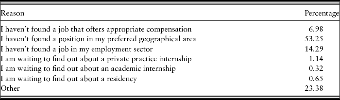
Every student was a graduating senior of an AVMA-accredited veterinary school. However, not all students had a pending job, which means not all had a starting salary to report. A distribution and list of reasons for not reporting a salary can be seen in Table 3. To address the selection bias from not reporting a starting salary, the two-step procedure of Heckman (Reference Heckman1976) was used.
Table 3. Reasons for Not Having a Starting Salary (N = 5,495)
The first stage of the Heckman procedure requires a probit regression, in which the probability that a given student has accepted a job offer and has a starting salary to report is estimated (Haines, Popkin, and Guilkey, Reference Haines, Popkin and Guilkey1988; Holcomb, Park, and Capps, Reference Holcomb, Park and Capps1995). From this information, an inverse Mills ratio for the ith student in year t is computed. All observations are used for the probit analysis, where the dependent variable equals one if the starting salary is nonzero and zero otherwise. Heckman (Reference Heckman1976) mathematically characterized the process. Denoting the normal cumulative density function by Φ, Heckman showed that
 $$\begin{equation}
{\rm{prob}}\left[ {{Z_{it}} = 0} \right] = 1 - {\rm{\Phi }}\left( {{W_{it}}{\delta _i}} \right),{\rm{\ }}i = 1, \ldots ,n;t = 1, \ldots ,T,
\end{equation}$$
$$\begin{equation}
{\rm{prob}}\left[ {{Z_{it}} = 0} \right] = 1 - {\rm{\Phi }}\left( {{W_{it}}{\delta _i}} \right),{\rm{\ }}i = 1, \ldots ,n;t = 1, \ldots ,T,
\end{equation}$$
where Wit is a vector of regressors related to having accepted a job offer, and δ i is the coefficient vector associated with these regressors. The regressors in the first stage include both individual and institution-based descriptive variables (i.e., age, gender, marriage status, number of children, self-employment status, amount of debt upon graduation, percentage of females and out-of-state students in graduating class, and availability of fellowships, residencies, and internships). The demographic variables are included in both stages of the regression as they are expected to affect actual starting salary values and the probability of reporting a salary. The institution-based variables are included only in the first stage as their effects cannot be isolated from the school fixed effects in the second stage. However, they are believed to contribute to the probability of reporting/having a starting salary as not every school will offer the same programs.
The first-stage provides estimates of the inverse Mills ratio (MRit ):
 $$\begin{equation}
{\widehat {MR}_{it}} = \left\{ {\frac{{\phi \left( {{W_{it}}{{\hat{\delta }}_i}} \right)}}{{1 - {\rm{\Phi }}\left( {{W_{it}}{{\hat{\delta }}_i}} \right)}}{\rm{\ for\ }}{Z_{it}} = 0} \right\},
\end{equation}$$
$$\begin{equation}
{\widehat {MR}_{it}} = \left\{ {\frac{{\phi \left( {{W_{it}}{{\hat{\delta }}_i}} \right)}}{{1 - {\rm{\Phi }}\left( {{W_{it}}{{\hat{\delta }}_i}} \right)}}{\rm{\ for\ }}{Z_{it}} = 0} \right\},
\end{equation}$$
where ϕ represents the probability distribution function. In the second stage, the inverse Mills ratio is used as an instrument that incorporates the latent variable (i.e., the predicted values from the probit model) into the estimation of the human capital model. Only observed values (i.e., nonzero responses) are used in the second-stage estimation (Park et al., Reference Park, Holcomb, Raper and Capps1996).
Given that each student has specific attributes associated with him/her, including the school attended, the following model is specified:
 $$\begin{equation}
S{S_{itj}} = \bm{X}_{\bm{itj}}^{'}\bm{\beta } + \mathop \sum \limits_{k = 1}^{27} {\alpha _{1k}}Schoo{l_{kj}} + {\lambda _i}\left( {\widehat {M{R_{itj}}}} \right) + {\eta _t} + {\varepsilon _{itj}},
\end{equation}$$
$$\begin{equation}
S{S_{itj}} = \bm{X}_{\bm{itj}}^{'}\bm{\beta } + \mathop \sum \limits_{k = 1}^{27} {\alpha _{1k}}Schoo{l_{kj}} + {\lambda _i}\left( {\widehat {M{R_{itj}}}} \right) + {\eta _t} + {\varepsilon _{itj}},
\end{equation}$$
where SSitj
denotes starting salaryFootnote
3
of veterinary student i in year t at school j;
Xijt
represents a vector of characteristics of veterinarian student i in year t; Schoolkj
represents indicator variables representing at which school the veterinarian received training;
 ${\widehat {MR}_{itj}}$
is the inverse Mills ratio; η
t
~ N(0, σ2
γ) denotes the random effect for year; and ε
itj
~ N(0, σ2
ε) denotes the general error term, where η
t
and ε
itj
are independent.
${\widehat {MR}_{itj}}$
is the inverse Mills ratio; η
t
~ N(0, σ2
γ) denotes the random effect for year; and ε
itj
~ N(0, σ2
ε) denotes the general error term, where η
t
and ε
itj
are independent.
The Heckman procedure is nonlinear, which allows the same variables to be used in both stages of the model. However, it is desirable to have variables that are specific to the first stage to give the inverse Mills ratio greater explanatory power. For this analysis, the demographic variables are used in both stages of the regression, whereas the school/institution-level characteristics (whether the veterinary program has a business program, the percentage of females and out-of-state students in the graduating class, and whether the school offers fellowships, residencies, and internships) and the amount of debt a veterinary student has upon graduation are only included in the first stage of the model. Variables only included in the second stage of the model are the schools and practice types, which are used as fixed effects. Also, because the data were collected from six different years, a year random effect is used. The use of school/institution-level characteristics in the first stage is to introduce heterogeneity into the model that cannot be captured simultaneously with the fixed effects in the second stage.
Because of the transformation of Heckman's approach, and the nature of the data, the Murphy and Topel (Reference Murphy and Topel1985) estimate of variance is used to correct for heteroscedasticity. Specifically, the estimated covariance matrix for the second-stage model needs to be adjusted to take into account the variability in the predicted variables from the first stage (Hole, Reference Hole2006). The Murphy-Topel estimate of variance for a two-step model is given by
 $$\begin{equation}
{\hat{V}_2} + {\hat{V}_2}\left( {\hat{C}{{\hat{V}}_1}{{\hat{C}}^{\rm{'}}} - \hat{R}{{\hat{V}}_1}{{\hat{C}}^{\rm{'}}} - \hat{C}{{\hat{V}}_1}{{\hat{R}}^{\rm{'}}}} \right){\hat{V}_2},
\end{equation}$$
$$\begin{equation}
{\hat{V}_2} + {\hat{V}_2}\left( {\hat{C}{{\hat{V}}_1}{{\hat{C}}^{\rm{'}}} - \hat{R}{{\hat{V}}_1}{{\hat{C}}^{\rm{'}}} - \hat{C}{{\hat{V}}_1}{{\hat{R}}^{\rm{'}}}} \right){\hat{V}_2},
\end{equation}$$
where
 ${\hat{V}_1}$
(q × q) and
${\hat{V}_1}$
(q × q) and
 ${\hat{V}_2}$
(p × p) are the estimated covariance matrices for model 1 and model 2, respectively, where each is the model-based estimate not taking into account that the estimate of the parameter vector in model 1 is embedded in model 2. Further,
${\hat{V}_2}$
(p × p) are the estimated covariance matrices for model 1 and model 2, respectively, where each is the model-based estimate not taking into account that the estimate of the parameter vector in model 1 is embedded in model 2. Further,
 $$\begin{equation}
\hat{C}{\rm{\ }} = {\rm{\ }}\left( {p{\rm{\ }} \times {\rm{\ }}q} \right){\rm{\ matrix\ given\ by\ }}\left\{ {\mathop \sum \limits_{i = 1}^n \left( {\frac{{\partial ln{f_{i2}}}}{{\partial \widehat {{\theta _2}}}}} \right){\rm{\ }}\left( {\frac{{\partial ln{f_{i2}}}}{{\partial \widehat {{\theta _1}{\rm{'}}}}}} \right)} \right\}
\end{equation}$$
$$\begin{equation}
\hat{C}{\rm{\ }} = {\rm{\ }}\left( {p{\rm{\ }} \times {\rm{\ }}q} \right){\rm{\ matrix\ given\ by\ }}\left\{ {\mathop \sum \limits_{i = 1}^n \left( {\frac{{\partial ln{f_{i2}}}}{{\partial \widehat {{\theta _2}}}}} \right){\rm{\ }}\left( {\frac{{\partial ln{f_{i2}}}}{{\partial \widehat {{\theta _1}{\rm{'}}}}}} \right)} \right\}
\end{equation}$$
 $$\begin{equation}
\hat{R} = {\rm{\ }}\left( {p{\rm{\ }} \times {\rm{\ }}q} \right){\rm{\ matrix\ given\ by\ }}\left\{ {\mathop \sum \limits_{i = 1}^n \left( {\frac{{\partial ln{f_{i2}}}}{{\partial \widehat {{\theta _2}}}}} \right){\rm{\ }}\left( {\frac{{\partial ln{f_{i1}}}}{{\partial \widehat {{\theta _1}{\rm{'}}}}}} \right)} \right\},
\end{equation}$$
$$\begin{equation}
\hat{R} = {\rm{\ }}\left( {p{\rm{\ }} \times {\rm{\ }}q} \right){\rm{\ matrix\ given\ by\ }}\left\{ {\mathop \sum \limits_{i = 1}^n \left( {\frac{{\partial ln{f_{i2}}}}{{\partial \widehat {{\theta _2}}}}} \right){\rm{\ }}\left( {\frac{{\partial ln{f_{i1}}}}{{\partial \widehat {{\theta _1}{\rm{'}}}}}} \right)} \right\},
\end{equation}$$
where f i1 and f i2 are observation i’s contribution to the likelihood function of models 1 and 2, respectively (Greene, Reference Greene2012).
Another potential source of heteroscedasticity comes from those reporting an expected self-employment income. These students do not have an actual salary offer from an employer and are most likely estimating their salary. To account for this issue, a multiplicative heteroscedasticity correction, with self-employed as the only variable, is included in the second stage of the Heckman procedure.
5. Results
Because a two-step estimation approach was used, the models from each step are presented. The probit model had a 70% correct prediction rate; Table 4 shows that most of the personal characteristics of the students and school-level variables significantly affect the probability of a student reporting a starting salary. Self-employed graduating students had a higher probability of reporting a starting salary, even if the reported salary was an estimate. This is intuitive as they are not pursuing offers from veterinary employers and should, therefore, have some preconceived salary expectation as a self-employed veterinarian. Students who are older, female, married, and have children all have lower probabilities of reporting a starting salary, which is consistent with previous literature (see Baliamoune-Lutz and McGillivray, Reference Baliamoune-Lutz and McGillivray2015; Battistón, García-Domench, and Gasparini, Reference Battistón, García-Domench and Gasparini2014; Brewer, Eide, and Ehrenberg, Reference Brewer, Eide and Ehrenberg1999). Debt level does not have a significant effect on the probability of reporting a starting salary, suggesting that the level of debt accumulated during veterinary school is not a factor in the hiring decisions of veterinary employers.
Table 4. Factors Affecting the Probability of Reporting a Starting Salary: Probit Estimates for the First-Stage Heckman Procedure (N = 14,957)

Note: Asterisks (*, **, and ***) denote statistical significance at the 0.10, 0.05, and 0.01 levels, respectively.
Some school-specific attributes, such as the percentage of females in the graduating class and whether the school offers fellowships, have positive effects on the probability of a graduate reporting a starting salary. Conversely, other school-specific traits such as the presence of a business program specific to the veterinary program, the percentage of out-of-state students, and the presence of residencies at the school lead to a lower probability of reporting a starting salary. The school-specific variable that was not significant was the presence of internships, which is not surprising because most schools offer or promote internships.
The mixed model results are shown in Table 5. The results reveal that almost all the school fixed effects are statistically different from the base institution (Western University), except for Michigan State University, Louisiana State University, Washington State University, and Iowa State University. More specifically, students at schools such as Colorado State University; Tufts University; Louisiana State University; Texas A&M University; Ohio State University; University of Minnesota; University of Missouri, Columbia; University of Pennsylvania; University of Tennessee; and the University of Wisconsin tend to have higher starting salaries compared with those at Western University. These starting salary differences control for the impacts of individual student characteristics and chosen practice area.
Table 5. Mixed Model of Veterinarian Starting Salary Estimates with School Fixed Effects in Thousands of Dollars (N = 9,429)

Note: Asterisks (*, **, and ***) denote statistical significance at the 0.10, 0.05, and 0.01 levels, respectively.
The inverse Mills ratio was used to account for censored response bias in the second-stage mixed model and was negative and statistically significant. This accounts for the bias that resulted from the nonresponse/selectivity of students who were unable/unwilling to report a starting salary. More specifically, the negative coefficient of the inverse Mills ratio represents the fact that students who are most similar to those who do not report a salary tend to have lower overall starting salaries.
Also shown in Table 5, four individual-level characteristics have a statistically significant effect on starting salaries: gender, whether the graduating senior is going to be self-employed, mean household income where the student will be practicing, and the age of the student upon graduation. Female graduates had lower reported starting salaries (by about $2,000), but reported starting salaries were higher for those who were self-employed (by about $28,400), older when completing the program (about $70 per year of age), and those locating in areas with a higher mean household income ($60 increase for every $1,000 increase in mean household income).
Students pursuing employment with the federal government, uniformed services, industry, and not-for-profit companies have statistically significant and higher starting salaries as compared with the base, which constitutes companion animal practices. Graduates pursuing a job in the areas of food animal and local government do not have starting salaries significantly different from those pursuing companion animal practices. Those working as equine practitioners average about $24,650 less in starting salary than those who start as companion animal veterinarians. On the other end of the spectrum, a graduate who accepts a job in private industry (e.g., animal genetics and pharmaceutical research) averages about $27,900 more than companion animal practitioners. As for the random error term for year, there is about $5,000 of variance in the estimates attributed to differences across years.
The mixed model results indicate differences in starting salaries between the 27 other schools and a base school, but to further define institutional differences, the least squares means (LSMEANS) of starting salaries by students from all schools were estimated (Table 6). LSMEANS are used as they adjust mean values across schools in relation to the other covariates within the mixed model and are more informative than a simple mean. From the LSMEANS, the average is $44,455 with the largest difference between schools at about $3,700. This difference is small compared with the full value of the starting salaries, suggesting that, at least in terms of graduates’ starting salaries, there is only a small benefit to choosing one veterinary program over another based solely on school reputation.
Table 6. Least Squares Means of Starting Salaries for all Schools (in thousands of dollars; overall mean = 46.54)

The reported starting salaries simple mean is lower than actual salaries reported in the AVMA Report on Veterinary Compensation (AVMA, 2015a). The mean salary across all veterinarians in private practiceFootnote 4 with 1 to 2 years of experience is $77,758 (in 2014 dollars). The simple mean of those employed in private practice within our sample is about $59,687. Because the mean reported in the 2015 AVMA Report on Veterinary Compensation includes those with an additional year of experience, it could be assumed that there are returns to experience and that those with only 1 year of experience may have a lower salary than the mean.
When comparing the two stages of the model, we see that that most of the student-level variables change sign from the probit regression to the mixed model. For example, increases in age lower the probability of having a starting salary but increase the actual value of the starting salary. This is also true for those who are married and have children, but none of the parameter estimates for these three variables were significant in the mixed model. On the other hand, whether the student is female and whether the student is to be self-employed retain the same parameter estimate signs. Specifically, females have a lower probability of reporting a starting salary and a lower overall starting salary, whereas those that are to be self-employed have a higher probability of reporting a starting salary and have a higher overall starting salary.
6. Summary and Conclusions
The AVMA slogan is “Our Profession. Our Passion.” The emphasis on passion is apparent in the choices made by veterinary students as the average reported starting salary at graduation is $47,000 within this study, which includes part-time and full-time employment. This emphasis on passion relative to economic incentives affects both starting salaries and lifetime earnings potential. The analysis of starting salary data shows statistically significant differences (albeit small) in starting salaries, less than $2,000, as a result of institutional choice. However, the greatest differentiating factor is the new veterinarian's choice of practice type with a range of about $53,000 in starting salary differences.
It is no surprise that a person's age, which is presumably a proxy for maturity and experience, and employment location have positive effects on starting salaries. Also, consistent with findings from previous literature, females tend to earn less than their male counterparts in similar positions. Note that this difference in income even exists for self-employed individuals as females make about $4,000 less than males. One possible explanation for this gender income inequality suggested by the AVMA Report on Veterinary Markets (AVMA, 2015b) is that female veterinarians sometimes choose to work fewer hours and thus have less compensation than male veterinarians.
The large difference in starting salaries from practice types supports suggestions from previous literature that market pressures (demand, supply, or both) are influencing incomes for veterinarians of specific practice types. For example, equine practitioners tend to have much lower starting salaries than their peers in other types of veterinary practice. Furthermore, a large portion of graduating veterinary medicine students across all schools (at least 28%) pursue additional education or employment with other (nontraditional) practices, which negatively affects their earnings immediately following veterinary school. The lower salary could be a result of being employed part-time (much like those pursing an internship or residency) or because they work fewer hours (but still considered full-time) while pursuing further education. Also, it is plausible that those pursuing further education incur income from being a graduate research/teaching assistant, thereby not being considered a full-time employee. In either case, this information is not explicitly stated within the survey. However, these decisions may be the result of veterinary “passion” or because the graduating veterinarians view greater future income potential from the experience gained in the lower-paying early years of their careers.
In general, this research adds to the growing literature on veterinary economics. Knowing potential earning differences across schools and practice types should help veterinary medicine professionals to assist veterinary medicine students with making more optimal decisions. This information may be especially beneficial in the South (i.e., the home of almost one-third of all recent veterinary school applicants and a region attractive to new, practicing veterinarians).
Although this study dealt specifically with veterinarian starting salaries, there is still some evidence (Dicks, Bain, and Knippenberg, Reference Dicks, Bain and Knippenberg2015) to support the idea of a greater long-term return for an obtained veterinary degree. Future research will examine the career earnings potential for veterinarians by specialty, interaction effects of practice types across schools, spatial effects of earning potential by practice type, practice-specific and geographically dispersed demand for veterinary services, and the impact of experiences (internships, residencies, and further education) on long-term income potential.


 Open access