


1. Overview and problem statement
Subsidy policies often are used to reduce income variability and risk of failure and ensure smooth supply of commodities in order to reduce uncertainties in agricultural markets (Goodwin, Mishra, and Ortalo-Magné, Reference Goodwin, Mishra, Ortalo-Magné, Zivin and Perloff2012). Common subsidy policies directed at farmers are deficiency payments, direct income support, crop insurance, and countercyclical payments. The federal government allocated $288 billion for agricultural subsidies from 2008 to 2012 under the 2008 Farm Bill (Zivin and Perloff, Reference Zivin, Perloff, Zivin and Perloff2012). The U.S. Department of Agriculture (USDA) announced subsidy payments of $4.7 billion to producers through the market facilitation program to address potential losses in 2018 associated with trade damages (USDA, 2018). Recent policies affecting the factor demand and purchase of agricultural commodities include subsidies related to biofuel production (Rajagopal and Zilberman, Reference Rajagopal and Zilberman2007; deGorter and Just, Reference de Gorter and Just2010).
Successfully meeting policy objectives of protecting producers from price volatility and smoothing supply of commodities depends on how much recipients benefit from subsidies used to achieve these goals. Subsidy incidence (i.e., the transfer of subsidy payments from intended recipients to other economic agents through market exchange) reduces the amount of intended income transfer to recipients and may undermine intended economic response. This deviation in intended income distribution can negatively affect policy effectiveness (Zivin and Perloff, Reference Zivin, Perloff, Zivin and Perloff2012). Moreover, subsidy incidence can create allocative inefficiency in the agricultural marketing chain through the creation of deadweight loss (Babcock, Reference Babcock, Zivin and Perloff2012). Hence, although these subsidy policies provide benefits, they may also cause unintended consequences and create efficiency and distribution concerns (Devadoss and Bayham, Reference Devadoss and Bayham2010).
Neoclassical theory suggests that in a perfectly competitive market, a per unit subsidy changes price and quantity traded and increases total earnings depending on the relative elasticity of supply and demand. The price change after a subsidy measures the degree of subsidy incidence. Given the assumption of a perfectly competitive market, the potential impacts of a subsidy and the degree of subsidy incidence can be estimated (Rosen and Gayer, Reference Rosen and Gayer2010).
Although market outcomes (i.e., equilibrium price, quantity traded, total earnings, buyer earnings, and seller earnings) may differ between competitive and imperfectly competitive markets, the theory of subsidy incidence applies to both (Rosen and Gayer, Reference Rosen and Gayer2010). Yet, empirical research suggests incidence predictions do not hold in imperfectly competitive markets, because the subsidy share shifts toward agents who hold market power (Goodhue and Russo, Reference Goodhue, Russo, Zivin and Perloff2012).
Much like market structure, trading institutionsFootnote 1 and delivery methodsFootnote 2 also affect market outcomes. For example, English auction and private negotiation trading institutions can affect relative competitiveness and bargaining power between buyers and sellers and result in market outcomes different from competitive markets, even when market supply and demand conditions are the same (Menkhaus, Phillips, and Bastian, Reference Menkhaus, Phillips and Bastian2003). Similarly, delivery methods can also affect relative bargaining power that influences market outcomes. Producers sell commodities before production in forward delivery markets but incur production cost before sale in spot markets (also called advance production). Spot delivery can create bargaining disadvantages for sellers as they try to reduce the risk of inventory loss during negotiation (Menkhaus, Phillips, and Bastian, Reference Menkhaus, Phillips and Bastian2003). As a result, market outcomes differ across these delivery methods given the same trading institution (Menkhaus, Phillips, and Bastian, Reference Menkhaus, Phillips and Bastian2003; Nagler et al., Reference Nagler, Bastian, Menkhaus and Feuz2015). Different combinations of trading institutions and delivery methods alone can result in deviations from predicted equilibria in perfectly competitive markets (Menkhaus, Phillips, and Bastian, Reference Menkhaus, Phillips and Bastian2003). Given the potential effect of trading institution and delivery method on market outcomes, subsidy incidence may also be affected by these market environment factors. Measuring policy effectiveness of subsidies requires understanding how subsidy incidence may interact with such market characteristics.
A traditional agricultural trading institution is auctions. However, privately negotiated trades are becoming more prevalent in agricultural marketing chains. Privately negotiated marketing and production contracts represent 52% of all livestock and 35% of all commodities as a share of the total value of U.S. agricultural production (MacDonald, Reference MacDonald2015). This shift in trading institution may be motivated by high uncertainty in agricultural production and associated risks with supply volatility. Both sellers and buyers may benefit from private negotiation as it allows each to manage price risks while allowing sellers to differentiate products and processors (commodity buyers) to manage stable and customized input supplies (Adjemian et al., Reference Adjemian, Brorsen, Hahn, Saitone and Sexton2016). This institution can also reduce marketing and transaction costs for all parties (Menkhaus et al. Reference Menkhaus, Phillips and Bastian2003; Nagler et al. Reference Nagler, Bastian, Menkhaus and Feuz2015).
Although private negotiation has its benefits, it also negatively affects producers’ pricing, bargaining behavior, and relative bargaining power. With more private negotiation, there are fewer reported market transactions, causing difficulty in price discovery (Plain and Grimes, Reference Plain and Grimes2006; Nagler et al., Reference Nagler, Bastian, Menkhaus and Feuz2015; Adjemian et al., Reference Adjemian, Brorsen, Hahn, Saitone and Sexton2016). The lack of market information can affect the relative bargaining power of buyers and sellers and negotiation outcomes (Katchova, Reference Katchova2010). Sellers have been found to receive lower prices in private negotiation than in auction markets, and lower quantities are traded than predicted (Menkhaus, Phillips, and Bastian, Reference Menkhaus, Phillips and Bastian2003; Menkhaus et al., Reference Menkhaus, Phillips, Bastian and Gittings2007). Also, incurring production cost before sale puts sellers at a bargaining disadvantage because of the risk of loss from unsold inventory, especially for perishable goods (Menkhaus el al., Reference Menkhaus, Phillips, Bastian and Gittings2007). As a result, advance production in spot markets creates downward pressure on price, and quantities produced and traded, particularly in a private negotiation institution. Menkhaus, Phillips, and Bastian (Reference Menkhaus, Phillips and Bastian2003) find sellers’ relative earnings are lowest in privately negotiated spot markets.
Given the prominence of private negotiation and advance production in agricultural commodity markets, understanding the impact of a subsidy in this market environment can improve policy design and effectiveness. Additionally, given previous findings of distinct impacts from trading institution and delivery method on market outcomes, competitive predictions regarding subsidy incidence likely do not hold in this market environment. However, the nature of private negotiation transactions causes a paucity of publicly available market data, limiting the potential for econometric analysis to isolate potential subsidy impacts (Nagler et al., Reference Nagler, Menkhaus, Bastian, Ehmke and Coatney2013). Therefore, experimental methods offer opportunities to investigate how a subsidy affects market outcomes in privately negotiated spot markets beyond what theory may provide. Our research objective is to evaluate subsidy incidence in this market environment using market experiments.
2. Subsidy incidence theory
A subsidy shifts the supply (demand) curve outward when the seller (buyer) receives the payment. The shift changes the equilibrium price and/or quantity traded depending on the initial relative elasticity of supply and demand. A price change because of a subsidy implies that subsidy recipients do not enjoy the total benefits of the payment, but rather share it with economic agents on the other side of the market. This transfer of subsidy benefits from the recipient to the other party through price changes is called subsidy incidence (Rosen and Gayer, Reference Rosen and Gayer2010). Subsidy incidence theoretically is independent of subsidy allocation (Rosen and Gayer, Reference Rosen and Gayer2010). Independence of subsidy allocation and distribution creates a difference between statutory (subsidy receipt by policy) and economic (actual distribution of subsidy) incidence. Based on liability side equivalence (LSE), economic incidence for subsidies is theorized to depend solely on the relative elasticity of supply and demand, independent of recipients (Ruffle, Reference Ruffle2005). As relative elasticities remain intact after introducing a subsidy, even in imperfectly competitive markets, subsidy incidence theories hold in imperfectly competitive markets as well (Rosen and Gayer, Reference Rosen and Gayer2010).
3. Relevant subsidy incidence literature
Given theory related to subsidy incidence, subsidy policies raise many efficiency and distribution concerns, motivating analyses investigating subsidy incidence. Goodwin, Mishra, and Ortalo-Magné (Reference Goodwin, Mishra, Ortalo-Magné, Zivin and Perloff2012) found that producer subsidies favor landowners renting or selling land as these subsidies increase land prices. This capitalization (i.e., transfer of producer’s subsidy into land value) results in price distortion and inefficient allocation of land resources. Moreover, these subsidies benefit old landowners at the cost of new owners, causing entry barriers, market concentration, and land market inefficiencies (Goodwin, Mishra, and Ortalo-Magné, Reference Goodwin, Mishra, Ortalo-Magné, Zivin and Perloff2012).
Although subsidy incidence is found in land markets, its degree does not conform to theory. As land is expected to have a perfectly inelastic supply, neoclassical theory suggests that any subsidy to producers, who demand land as a factor of production, should result in full incidence of the subsidy to the landowners. Using firm-level land rental data for producers, Kirwan (Reference Kirwan2009) found only 25% payment incidence to the landowners in the land rental market compared with 100% incidence suggested by theory. However, the estimation did not control for different land qualities to segregate the variation in land rental value arising from land qualities and subsidy incidence. With a refined analysis addressing aggregation issues and controlling for land quality, even lower incidence (between 14% and 24%) has been found (Kirwan and Roberts, Reference Kirwan and Roberts2016).
Goodhue and Russo (Reference Goodhue, Russo, Zivin and Perloff2012) found in the imperfectly competitive flour milling industry, where there are a limited number of millers relative to many wheat producers, millers pay lower prices for wheat when producers receive deficiency payments, increasing their marketing margin by 10%. Along with relative elasticity, market power contributes to the size of subsidy incidence.
These empirical investigations, however, have limitations. First, these studies do not consider the impacts of different trading institutions and delivery methods on subsidy incidence. Yet, as described, these factors have significant impacts on market outcomes (Menkhaus, Phillips, and Bastian, Reference Menkhaus, Phillips and Bastian2003). Second, given the nature of privately negotiated transactions, data for empirical analyses are often not available (Nagler et al., Reference Nagler, Menkhaus, Bastian, Ehmke and Coatney2013). Moreover, in naturally occurring markets, many factors interact with each other and confound empirical estimates of market impacts from subsidies. Experimental markets can overcome these limitations by offering a controlled environment. With appropriate incentives and design, participants in controlled experiments exhibit real-world economic behavior (Davis and Holt, Reference Davis and Holt1993). Thus, experiments allow for control of extraneous factors and generate reliable data for examining subsidy incidence.
Previous market experiments that study a subsidy (and/or tax) indicate that payment incidence can vary with trading institutions and delivery methods (Ruffle, Reference Ruffle2005; Nagler et al., Reference Nagler, Menkhaus, Bastian, Ehmke and Coatney2013). Ruffle (Reference Ruffle2005) shows in competitive auction market experiments that price converges to the predicted competitive equilibrium when a tax or subsidy is introduced, resulting in tax or subsidy incidence equal to predicted incidence (Ruffle, Reference Ruffle2005). As a result, the author argues competitive forces offset any impact of noneconomic factors, such as framing effects.Footnote 3 Yet, Kerschbamer and Krichsteiger (Reference Kerschbamer and Kirchsteiger2000) show in ultimatum game experiments (which represent bilateral negotiated outcomes) that even under conditions representing perfectly competitive outcomes, social norms affect tax incidence, implying a moral obligation to bear the tax that violates LSE. Both Ruffle (Reference Ruffle2005) and Kerschbamer and Krichsteiger (Reference Kerschbamer and Kirchsteiger2000) recognize that violation of LSE is more plausible in imperfectly competitive markets.
Alternatively, Nagler et al. (Reference Nagler, Menkhaus, Bastian, Ehmke and Coatney2013) find less than 25% incidence is observed in privately negotiated forward markets (where buyers, mimicking producers receiving a subsidy, act as factor purchasers), whereas the competitive model predicts 50% incidence. The authors posit a sense of fairness and same-side competition may affect subsidy incidence in private negotiation. They hypothesize that sellers may behave as if it were “fair” for buyers to keep a higher proportion of the subsidy because it was given to them. Higher same-side competition among the recipients of a subsidy should also increase subsidy incidence, whereas higher same-side competition among the nonrecipients should reduce it. If buyers were to receive a subsidy for each unit they traded, this should effectively shift out the redemption value or demand curve, making each unit potentially more valuable, driving up competition among buyers to purchase units. The opposite would be true if sellers were to receive the subsidy, effectively reducing unit costs or shifting out supply curves, and potentially increasing the competition among sellers to sell units in order to receive more subsidy benefits. In privately negotiated forward markets, Menkhaus et al. (Reference Menkhaus, Phillips and Bastian2003, Reference Menkhaus, Phillips, Bastian and Gittings2007) find reduced quantities produced and traded relative to the predicted equilibrium because of matching risk. This reduced production creates same-side competition among buyers to purchase units. However, when subsidies were publicly given to buyers, it seemed to mitigate this competition and contributed to lower prices, lower incidence, and higher relative earnings compared with predicted levels (Nagler et al., Reference Nagler, Menkhaus, Bastian, Ehmke and Coatney2013).
Research also shows evidence of framing effects in privately negotiated market environments. Nagler et al. (Reference Nagler, Menkhaus, Bastian, Ehmke and Coatney2013) test whether market outcomes are the same when all participants are told of the buyer receiving a per unit subsidy or when the buyers have their redemption schedules (the amount for which a buyer could redeem each unit purchased) privately shifted by an amount equal to the subsidy. Buyers actually paid higher prices on average when their redemption schedules were shifted, as prices increased to a level near the predicted equilibrium, leading to 87% of the predicted incidence level. This result suggests different incidence behavior when the increase in redemption values is framed as a subsidy rather than the result of an equal shift in the redemption value (demand) schedule for buyers.
Subsidy impacts on units produced and traded may not be as predicted in markets dominated by private negotiation and spot delivery. The impact on quantities traded from subsidies is lower in privately negotiated forward markets than that expected in competitive markets (Nagler et al., Reference Nagler, Menkhaus, Bastian, Ehmke and Coatney2013). Moreover, quantities produced and traded in spot markets are well below levels observed in privately negotiated markets with forward delivery (Menkhaus et al., Reference Menkhaus, Phillips and Bastian2003). Thus, although subsidies incentivize production, advance production risks may reduce subsidy impacts on production and result in less than competitive trade levels.
Existing research on subsidy incidence, however, has not investigated the impact of subsidies on bargaining behavior and market outcomes in privately negotiated spot markets. As shown in other research, theory is likely not to accurately describe behavior in this environment. Because of the presence of matching risk and inventory loss risk to sellers in this market environment that affects price, production, and trade outcomes (Menkhaus et al., Reference Menkhaus, Phillips and Bastian2003, Reference Menkhaus, Phillips, Bastian and Gittings2007), the effects of a per unit subsidy are not easily predicted. Given the growing importance of private negotiation in the agricultural marketing chain, the lack of research, and the potential disparity in predicted outcomes, we investigate market outcomes in privately negotiated spot markets affected by subsidies and measure subsidy incidence using experimental economics. Specifically, we test the following hypotheses:
1. H0: There is no difference in subsidy incidence between privately negotiated spot markets and predicted competitive market outcomes.
2. H0: Subsidy-incidence equivalence holds in privately negotiated spot markets.
3. H0: Subsidy incidence is equivalent when an income transfer is framed as a subsidy versus being represented as an equivalent shift in the redemption value schedule for buyers or unit cost schedule for sellers, in privately negotiated spot markets.
4. H0: Subsidy impacts on quantities traded do not vary between privately negotiated spot markets and predicted competitive market outcomes.
4. Methods
We use experimental markets to achieve our research objectives and test our proposed hypotheses. Participants were recruited from a college campusFootnote 4 to participate in the experimental markets. Different participants were used for each experimental session to address issues caused by using the same participants across multiple replications (Charness, Gneezy, and Kuhn, Reference Charness, Gneezy and Kuhn2012). For each experimental session, four buyers and four sellers were recruited to allow for one-to-one trading on a computer network.
We followed standard experimental procedures and provided instructions and a practice session to ensure participants understood what they needed to do in the experiment (Davis and Holt, Reference Davis and Holt1993; Friedman and Sunder, Reference Friedman and Sunder1994). Instructions were presented explaining the basics of the experiment, trading rules, how buyers and sellers make trades, how buyers and sellers make a profit, examples of how profits are calculated, any necessary specifics regarding subsidy treatments, and example trading screens (instructions available upon request). Once participants had questions answered and were aware of procedures, participants were randomly assigned as either buyers or sellers when they logged into the computer. Each participant remained in this role throughout the experimental session. When participants logged in and learned their role, they saw either a supply schedule (sellers receive a unit cost schedule) or a demand schedule (buyers receive a redemption value schedule). Subjects then participated in a practice session using unit cost or redemption value schedules different from the actual experiment to familiarize them with the experiment. During the practice session, questions were encouraged and answered, regarding such things as market procedures, how to make bids or offers, how to make money, and how profits were calculated. Practice trading periods were conducted until all participants indicated they were ready to move to the real experiment.
Once the practice session concluded, the real experiment began, and buyers and sellers traded the homogenous product called “units” in order to earn tokens.Footnote 5 For sellers, earnings in each trading period were based on the price(s) for which they traded their individual unit(s) minus the unit cost(s) to produce the unit(s) sold (see Table 1 for the unit cost schedule in the no-subsidy treatment). For example, if a seller traded units 1 and 2 for 78 and 80 tokens, respectively, the seller would have earned 88 tokens on those two trades (unit 1: 78 − 30 = 48; unit 2: 80 − 40 = 40). Earnings for buyers were based on the redemption value they received for the unit(s) purchased minus the negotiated price(s) they paid (see Table 1 for the redemption value schedule in the no-subsidy treatment). For example, if a buyer traded units 1 and 2 for 78 and 80 tokens, respectively, the buyer would have earned 92 tokens on those two trades (unit 1: 130 − 78 = 52; unit 2: 120 − 80 = 40). Similar to what we would expect in actual markets dominated by private negotiation, individuals trading in the market only knew about their individual unit values in their respective schedules. Sellers saw their own unit cost schedules when trading, but did not know other sellers’ unit costs or buyers’ redemption values. Similarly, buyers only saw their own redemption value schedules when trading.
Table 1. Seller and buyer schedules for different treatments

After each trading period, participants saw their profits earned in that period, and their accumulated earnings, before moving into the next trading period. At the end of the experiment, participants received a cash payoff equal to the sum of their profits earned during the experiment plus an initial endowment. Total earnings for individual participants ranged between $20 and $80 depending on individual performance in the respective treatments. Each experimental session concluded in approximately 2 hours.
Each session included 20 or more trading periods,Footnote 6 which consisted of a production decision by sellers followed by three 1-minute bargaining rounds.Footnote 7 In each bargaining round, randomly matched buyers and sellers bilaterally negotiated over price until an agreement was reached and a trade occurred, after which, negotiation began on the next unit. Buyer and seller pairs could trade as many units as they found profitable in a bargaining round. Individual buyers and sellers could trade up to a maximum of eight units during a trading period. Random matching of buyers and sellers during each bargaining round, with no other allowed communications except trading information during the experiment, averted the influence of reputation building and partner choosing (Phillips et al., Reference Phillips, Nagler, Menkhaus, Huang and Bastian2014). Additionally, units traded, trade prices, and payoffs were not made public to be consistent with the private negotiation institution. An improvement rule indicating bids must become progressively lower while offers must become be progressively higher was presented during the instructions and enforced during bargaining in the experimental session.
No inventory carryover was allowed to reflect advance production risks. Sellers lost the units produced (and their respective unit costs of production) but not traded after each period. This inventory loss created advance production risks for sellers in our experiment that parallel what sellers in agricultural commodity markets face (i.e., producers sink production costs into what they produce before they sell their product). Although buyers as processors may face input-requirement risks in real-life privately negotiated spot markets, we do not introduce such additional risks to isolate the impacts of advance production risks.
To test our hypotheses, five treatments (no subsidy, seller subsidy, buyer subsidy, seller revised schedule, and buyer revised schedule) were conducted with five replications (sessions) each, for a total of 25 replications. The no-subsidyFootnote 8 treatment provides a baseline for market outcomes in a privately negotiated spot market. Sellers traded based on the unit cost schedule labeled “no-subsidy seller schedule,” and buyers traded based on the redemption value schedule labeled “no-subsidy buyer schedule” in Table 1. In the two subsidy treatments, either sellers or buyers received a 20 token per unit subsidyFootnote 9 for each unit traded. All participants in these experiment sessions were made aware of this subsidy information in the instructions, and the respective subsidy was instituted and mentioned again during the practice session for further reenforcement of the subsidy treatment. For the seller subsidy treatment, the following was stated in the instructions: “In this experiment an additional per unit subsidy of 20 tokens will be paid to each seller on each unit traded at the end of each trading period.” A similar statement was made in the instructions for the buyer-subsidy treatments. This subsidy effectively shifts the base unit costs (no-subsidy seller schedule) or redemption values (no-subsidy buyer schedule) by 20 tokens for each unit as noted in Table 1 (labeled as per unit subsidy seller or per unit subsidy buyer, respectively). The revised schedule treatments either reduced unit costs for sellers by 20 tokens (seller revised schedule) or increased the unit redemption values by 20 tokens for buyers (buyer revised schedule) compared with the no-subsidy schedules (Table 1). To test framing effects, these changes in the schedules were not announced to participants in the experiment. That is, buyers or sellers just saw their respective altered schedule during their trading. This was done to test whether a change in observed incidence from the base treatment was a result of altered schedules alone or the public knowledge that some market participants received a “subsidy,” which effectively shifted seller or buyer schedules.
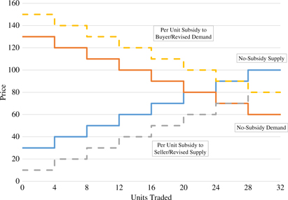
The use of consistent supply (unit cost) and demand (redemption value) schedules across sessions for each treatment (Table 1), allows us to sum across individuals and predict competitive equilibriums, as well as test for potential deviations in privately negotiated spot markets. The schedules result in discrete step functions of aggregate supply and demand in our laboratory market (Figure 1). Predicted equilibrium price in the no-subsidy treatment is 80 tokens (Table 2, Figure 1). The equilibrium price increases by 10 tokens, to 90 tokens, in the buyer subsidy and revised schedule treatments and decreases by 10 tokens, to 70 tokens, in the seller subsidy and revised schedule treatments (Table 2, Figure 1). These discrete step functions create a “quantity tunnel” resulting in a range of units traded at equilibrium (20–24 units for the no-subsidy treatment and 24–28 units for all other treatments). Relative earnings (buyers’ earnings minus sellers’ earnings) are predicted to be zero, with equal buyer and seller earnings of 150 and 210 tokens in the base and other treatments, respectively (Table 2). Together buyers and sellers can earn a total of 1,200 tokens in the base treatment (given schedules for buyers and sellers), which increases by 480 tokens in all other treatments.
Table 2. Predicted equilibria in different treatments


Figure 1. Aggregated supply and demand functions for different treatments.
5. Analysis
Data on price, quantity traded, total earnings, buyer earnings, and seller earnings for each trading period and treatment were collected. We adopt a parametric convergence model developed by Noussair, Plott, and Riezman (Reference Noussair, Plott and Riezman1995) to estimate each variable’s converged level for each treatment. The model is as follows:
 $$Z_{it} = {B_0}\left[{(t - 1)\over {t}} \right] + {B_1}\left({{1}\over {\rm t}} \right) + \sum\nolimits ^{i - 1} _{j = 1}{\alpha_j}{D_j}\left[{{(t - 1)}\over {t}}\right] + \sum\nolimits ^{i - 1} _{j = 1}{\beta_j}{D_J}\left({{1}\over{t}}\right) + {u_{it}},$$(1)
where Zit is the observed variable of interest such as price, number of units traded, or earnings for treatment i for each trading period t; B 0 is the predicted asymptote and B 1 is the starting level for the baseline treatment (no-subsidy); α j and β j are adjustments to the base treatment asymptotes (B 0) and starting (B 1) levels for each of j variable treatments; and D is the dummy variable representing the j th treatment (equal to 0 for the baseline and 1 for the rest).
As seen from equation (1), the convergence model is not a causal model. The model estimates parameters related to the observed path of the variable of interest across trading periods by using the number of the trading period for weighting. B 0 (the asymptote) weights later periods more heavily than earlier periods (because B 0 is multiplied by [t − 1/t]), and B 1 (the starting value) weights earlier periods more heavily (because B 1 is multiplied by [1/t]). For example, if in period 1 of the base treatment, we observe a price of 79 tokens, the prediction for the starting value in period t = 1 would be equal to 79 (because Zit = 79 = [(B 0) × (1 − 1/1)] + [(B 1) × (1/1)] + [0 for each of the indicator variable coefficients] = B 0 × 0 + B 1 × 1 + 0, then B 1 = 79). In period 20, the estimate of B 0 would be weighted by 0.95, and B 1 would be weighted by 0.05 for the observed level of Zit. Parameter estimates (αj, βj) are estimates of the difference in asymptotic and starting values in the base treatment to each other treatment’s estimated asymptotic and starting values (e.g., αj is the estimated difference in the asymptotic value of the variable between the base treatment B 0 and treatment j). These parameters allow estimation of the difference across each treatment compared to the base treatment (no subsidy) (i.e., test for differences between B 1 and [B 1 + βj] and between B 0 and [B 0 + αj] of each variable of interest). To understand the expected level of a variable of interest after the market reaches equilibrium, we utilize the estimates from the convergence model for the asymptote (reported in Table 3).
Table 3. Estimates for market outcomes across treatments
a Buyer earnings are normally distributed, so we report convergence estimates for this variable, but seller earnings are not normally distributed, so we report averages over the last five periods and use the Wilcoxon rank-sum statistic to test statistical significance.
b Net gain is defined as change in total earnings for the subsidy versus base treatment, minus subsidy payments. Total earnings minus subsidy payments are not normally distributed, and thus, we report averages over the last five periods and use the Wilcoxon rank-sum statistic to test statistical significance.
c Inventory loss is defined as production minus units traded. Because production is not normally distributed, we report average inventory loss over the last five periods of each treatment and use the Wilcoxon rank-sum statistic to test statistical significance.
Notes: Asterisks (***,**,*) indicate different from competitive predictions at the 1%, 5%, or 10% significance level, respectively. Different letters (A-C) indicate pairwise significant difference between treatments at 10% significance level. Number signs (###,##) indicate significantly different from 0 at 1% or 5% significance level, respectively.
To test our hypotheses, we focus on central tendencies across treatments. We construct a balanced panel using data from trading periods 1 through 20. The average of the data across each replication for each treatment is used to minimize individual influences in experimental sessions.Footnote 10 Thus, our panel data set consists of 100 observations (20 time-series observations for each of the five cross sections or treatments). Panel data are often both serially and contemporaneously correlated, and the residuals for this type of data set may not be homoscedastic (Parks, Reference Parks1967). Given our balanced panel data set, we use the Parks (Reference Parks1967) estimation technique to account for these three issues simultaneously, consistent with previous literature (e.g., Menkhaus et al., Reference Menkhaus, Phillips and Bastian2003, Reference Menkhaus, Phillips, Bastian and Gittings2007; Nagler et al., Reference Nagler, Menkhaus, Bastian, Ehmke and Coatney2013).
Wald tests and t-tests are used to evaluate statistically significant differences between converged values for different treatments and test our hypotheses. We compare asymptote estimates to their predicted levels using Wald tests. We use t-tests to compare parameter estimates for the asymptotes across treatments to evaluate whether treatment effects are significant. We test whether there is a statistically significant difference between the base treatment asymptote estimate (B 0) and the parameter of the base treatment asymptote plus the estimated adjustment for the treatment of interest (αj). Both the Wald test and t-test require data to be normally distributed (Berry and Lindgren, Reference Berry and Lindgren1996). We conducted the Shapiro-Wilk test to determine if the assumption of normality is met at the 5% significance level. If the variable of interest is found to not be normally distributed, we test whether the variable is severely skewed as defined by Brown (Reference Brown1997). If a variable fails the normality test and is severely skewed, a parametric test, such as the t-test cannot be used. In these cases, we report the variables’ average over the last five periods (period 16–20) for each replication and use Wilcoxon’s nonparametric rank-sum statistic to test for statistically significant differences of averages between treatments (Berry and Lindgren, Reference Berry and Lindgren1996).
6. Results
6.1. Subsidy impacts on price
Figure 2 shows the trend for price in each treatment. The “no-subsidy” (base treatment) price is consistently lower than the predicted level of 80 tokens and generally lies between seller subsidy and buyer subsidy prices. Subsidy and revised schedule treatment prices converge to the same levels, although from opposite directions. Prices in the no-subsidy seller schedule and the seller revised schedule treatments seem to approach their respective levels after the third trading period, whereas the per unit subsidy buyer schedule and buyer revised schedule prices do not converge until period 10.
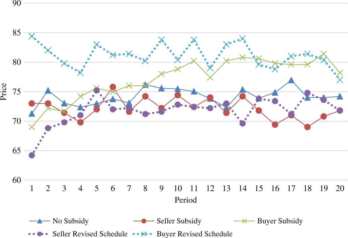
Figure 2. Price trends across treatments.
Empirical estimates tend to support the graphical analysis (see Figure 2). As expected, because of advance production risk and previous findings, the asymptotic value of price (i.e., convergence estimate, B 0) in the base treatment is nearly 5 tokens lower than the predicted level of 80 tokens (see Table 3) (Menkhaus, Phillips, Bastian, Reference Menkhaus, Phillips and Bastian2003; Menkhaus et al., Reference Menkhaus, Phillips, Bastian and Gittings2007). As expected, compared with price in the base treatment, the seller subsidy treatment reduces price but does so by nearly 3 tokens. A buyer subsidy increases it about 4 tokens. These prices are also significantly different from the predicted competitive equilibriums. Revised schedule treatment prices converge to the same level as their respective subsidy treatments (see Table 3), suggesting similar impacts on price when having a subsidy framed as a “per unit subsidy” compared to having it represented as a shift in a respective schedule.
These results imply that subsidy impact (either framed as a subsidy or a shift in the schedule) on price is different in privately negotiated spot markets from the competitive market predictions. As a result, compared with a 50% predicted subsidy incidence (i.e., 10 tokens out of a 20 token subsidy), only 14% (about 3 tokens, e.g., price of 74.76 tokens in the base treatment versus 72.02 tokens in the seller subsidy treatment) of the subsidy is transferred to buyers when sellers receive it. When buyers receive a subsidy, sellers get 21% (about 4 tokens, e.g., 74.76 in the base versus 79.01 in the buyer subsidy treatment) of that subsidy (Table 3). These findings confirm our hypothesis that subsidy incidence in privately negotiated spot markets is different from competitive market predictions independent of subsidy recipient.
The bargaining advantage of buyers over sellers, because of advance production risk faced by sellers, results in varying subsidy impacts depending on who receives the subsidy. The sellers’ bargaining disadvantage motivates them to keep more of a subsidy they receive to compensate for the potential losses incurred from unsold inventory. We believe a seller subsidy (in the form of either a subsidy or a shift in the supply schedule) mitigates seller risks and allows them to negotiate prices more aggressively, as prices are above the predicted equilibrium price.
Alternatively, in the buyer subsidy treatment, buyers give up approximately 21% of the subsidy to sellers (not statistically different from the buyer revised schedule treatment). Initially, this result might seem to suggest that either buyers are willing to give up more of the subsidy on average or sellers facing advance production risk might be bargaining more aggressively for the subsidy in this treatment. However, this incidence level is not statistically different from the seller subsidy treatments.Footnote 11 It is interesting to note this incidence level is much lower than that found in Nagler et al. (Reference Nagler, Menkhaus, Bastian, Ehmke and Coatney2013) when buyers were subsidized in a private negotiation forward delivery market environment.
Pairwise comparisons of incidence in all nonbase treatments with their predicted level of 50% support rejection of subsidy-incidence equivalence because prices in all subsidy treatments are statistically significantly different from each party receiving 50% of the subsidy. The subsidy recipients always keep a higher share of the subsidy payments. Thus, we conclude that subsidy-incidence equivalence does not hold in this market setting, and contrary to theoretical prediction, incidence equivalence is not independent of market institution and delivery method.
6.2. Subsidy impacts on trade
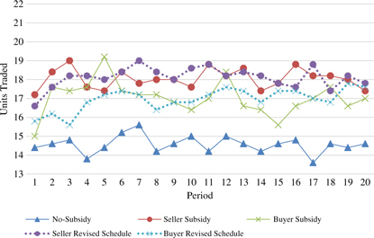
Graphical analysis of the trade data (Figure 3) offers less obvious differences across treatments than with prices. Units traded in the no-subsidy treatment are clearly below all the other treatments, suggesting a subsidy or revised schedule does cause the number of units traded to increase compared with no subsidy. Units traded in the no-subsidy treatment are estimated at 14.57 for the asymptote, significantly different than the approximately 18 or 17 units traded in the buyer or seller treatments, respectively (Table 3). As expected from the graphical analysis (Figure 2), all trade levels in the subsidy and revised schedule treatments are significantly different from the no-subsidy or base treatment as well (denoted by letters in comparisons across treatments in Table 3).
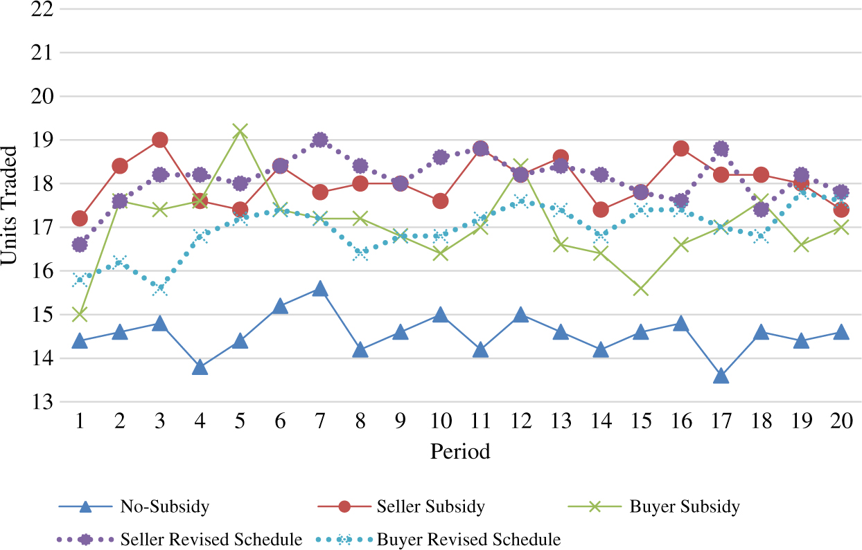
Figure 3. Trends in units traded across treatments.
Even though the subsidy, either buyer or seller, should create a level of trades at 24 to 28 units, this is not achieved in our market setting. Although the number of trades significantly increases in the buyer and seller treatments compared with the base, the number of trades observed from these treatments is about 6 to 10 trades fewer than the number predicted by theory (second row of Table 3 compared with second column of Table 2). These results highlight the interaction between subsidy and market environment as it relates to trade quantities. Furthermore, these findings confirm our expectation that subsidy impacts on units traded are different in privately negotiated spot markets than competitive market prediction (Table 3). Lower production and trade in privately negotiated spot markets reflect sellers trying to mitigate advance production risks by reducing the chance of inventory loss. With inventory loss, sellers lose production costs from their most expensive units when untraded, lowering their earnings.Footnote 12 Sellers learn to reduce units produced; yet the risk of losing untraded units continues to give the bargaining advantage to buyers. This bargaining advantage likely explains why trade prices are well below predicted levels in the buyer subsidy and buyer revised schedule treatments. Even though the reduced number of units being traded should increase potential same-side competition among buyers for units, that effect is apparently not large enough to increase prices and incidence levels to those predicted given sellers’ weak bargaining position.
6.3. Subsidy impacts on earnings
Buyers generally earn more than sellers in this market as can be seen in Table 3. Sellers only earn more than buyers in the seller treatments. Sellers earn 180.32 tokens in the seller subsidy treatment and 200 tokens in the seller revised schedule treatment compared with estimated buyer earnings of 163.65 and 165.42, respectively. Estimated average agent earnings are significantly different from the predicted level in all but the revised schedule treatments. Thus, although relative elasticity in our market experiments predicts a 50% incidence and equal earnings for buyers and sellers, the market environment affects the distribution of earnings.
The earnings disparity between buyers and sellers, even with reduced production and trade, implies that advance production risk greatly affects market outcomes when subsidies are in place compared with predictions. A subsidy to sellers in this market environment, at least in part, mitigates inventory loss risks given subsidized unit costs and seems to alter sellers’ relative bargaining power, resulting in slightly higher than predicted prices coupled with more units traded, and lower incidence than predicted. This ultimately improves sellers’ relative earnings. When buyers receive the subsidy, even in the face of fewer units traded than predicted levels, buyers do not seem to compete heavily for units but rather continue to enjoy a favorable bargaining environment, and prices are well below predicted levels. This allows buyers to keep the majority of the subsidy, as they give up nearly the same proportion of the subsidy as sellers when they receive the subsidy.
6.4. Subsidy impacts on total earnings
The convergence estimate of total earnings in the base treatment is nearly 970 tokens. This estimate is 230 tokens below the predicted 1,200 tokens and is statistically significant (Table 3). Earnings in all other treatments are significantly higher than the base treatment but significantly below the predicted level of 1,680 tokens. Earnings in the subsidy treatments range from 1,375 to 1,388 tokens (not statistically different from each other), about 300 tokens lower than the predicted level, but more than 400 tokens higher than observed in the base treatment (Table 3).
Subsidies increase total welfare in this market as predicted by theory but generate lower total earnings than competitive predictions. This market environment only generates 80%–88% of the total surplus available (Table 2), with or without a subsidy (Table 3). This supports findings from previous literature that privately negotiated markets are commonly less efficient and generate lower surplus than perfectly competitive markets with the same supply and demand conditions, even with a subsidy (Menkhaus, et al., Reference Menkhaus, Phillips and Bastian2003; Nagler et al., Reference Nagler, Menkhaus, Bastian, Ehmke and Coatney2013).
Public finance literature suggests that subsidy policies create allocative inefficiency and deadweight loss through subsidy impacts on price and quantity, but their impact on an already inefficient market is ambiguous (Rosen and Gayer, Reference Rosen and Gayer2010). Given the supply and demand schedule in our subsidy experiments, predicted trades are 24–28 units, which entails a subsidy payment between 480 and 560 tokens. This subsidy payment, in turn, increases predicted surplus by 480 tokens (Table 2). As a result, a deadweight loss between 0 and 80 tokens is expected. Although our market setting is inefficient in generating surplus, we find subsidies result in small but statistically significant positive net gains in welfare for the subsidy treatments (57.3 for seller subsidy and 60.4 tokens for buyer subsidy; Table 3). Although a subsidy creates deadweight loss in theory, our results suggest subsidies in privately negotiated spot markets reduce some of the inherent inefficiency given the institution and delivery method for this market environment, as the gains generated from the subsidy outweigh total subsidy payments.
6.5. Framing effects
We find little evidence of framing effects, as results in the subsidy and respective revised schedule treatments indicate there are no significant differences between subsidy and revised schedule treatment results for price, trades, and relative earnings (Table 3).Footnote 13 These findings differ from those reported by Nagler et al. (Reference Nagler, Menkhaus, Bastian, Ehmke and Coatney2013), who found evidence of framing effects in a private negotiations institution with forward delivery when buyers received a subsidy. However, we contend that rather than the nonexistence of a framing effect, it is plausible that these effects are potentially muted or offset by the dominant impact of advance production risk. Comparison of total earnings in subsidy treatments and revised schedule treatments shows that, although buyer subsidy and buyer revised schedule treatments generate the same level of earnings, the seller revised schedule treatment generates significantly higher (85 tokens) earnings than the seller subsidy treatment. In a market setting, where sellers are disadvantaged when bargaining, this result might have significant policy implications.
7. Summary and conclusions
Given uncertainties in agricultural commodity markets, subsidies primarily aim to increase and stabilize incomes and ensure consistent supply of commodities. Effectiveness of policies designed to meet these objectives depends on the magnitude of subsidy incidence, which, in turn, relates to resulting subsidy impacts on market outcomes. Our laboratory market experiments confirm our hypothesis that subsidy incidence in privately negotiated spot markets differs from competitive market predictions. About 14% of the subsidy is transferred to the buyers when received by sellers, and sellers receive 21% of the subsidy given to buyers. These levels are statistically lower than the competitive prediction and not statistically significantly different from each other. Thus, contrary to theory, subsidy-incidence equivalence does not hold in this market setting. Our results find fewer units traded and lower total earnings than predicted from competitive markets, implying reduced efficiency across all treatments, consistent with previous findings related to efficiency for this market setting (Menkhaus, Phillips, and Bastian, Reference Menkhaus, Phillips and Bastian2003; Menkhaus et al., Reference Menkhaus, Phillips, Bastian and Gittings2007). These results have significant implications for welfare, efficiency, and distribution impacts of subsidies in privately negotiated spot markets.
Incidence equivalence theory suggests that payment incidence is independent of statutory incidence, and thus, given the predicted outcomes, alternative policies should be assessed in terms of implementation costs only (Ruffle, Reference Ruffle2005; Rosen and Gayer, Reference Rosen and Gayer2010). Our findings against incidence equivalence in privately negotiated spot markets imply that not only competitiveness in the market but also relative bargaining strength, because of varying market institutions, affects incidence equivalence. Therefore, assessing policy alternatives requires consideration of the targeted beneficiaries, market institutions, and respective payment incidence to avoid unintended and inefficient subsidy allocation.
An additional implication from our research relates to that of potential behavioral anomalies affecting subsidy incidence. Previous research indicates an income transfer policy that is publicly presented as a subsidy results in different incidence levels than when the transfer was received by factor buyers as a shift in redemption values (Nagler et al., Reference Nagler, Menkhaus, Bastian, Ehmke and Coatney2013), suggesting a framing effect. Our research finds no such effect, as we find similar incidence levels across both buyers and sellers receiving the income transfer as a public subsidy or as a corresponding shift in redemption values or unit costs, respectively. We believe this result further accentuates the potential impact of the added risk from advanced production in the private negotiation spot market environment compared with that modeled in Nagler et al. (Reference Nagler, Menkhaus, Bastian, Ehmke and Coatney2013).
Advance production risks cause bargaining disadvantages for sellers in privately negotiated spot markets and result in an unequal distribution of earnings. Earnings disparity between buyers and sellers is mitigated by a subsidy to sellers and creates the most equal distribution of earnings among the policy alternatives considered in our study. However, inefficiency and lower trade levels result in lower than predicted seller earnings even with a seller subsidy. As a result, competitive prediction overestimates subsidy impacts on sellers’ income. On the contrary, a subsidy to buyers creates the highest earnings disparity given buyers’ already favorable bargaining position. Thus, competitive prediction overestimates subsidy impacts on sellers’ income whereas it underestimates buyers’ income when the subsidy is given to the buyer. These results suggest the actual income effect of a subsidy is different from the expected level. Alternatively, as subsidy policies result in fewer trades than predicted in this market, competitive prediction would overestimate the subsidy impacts on production and trade.
All these inefficiencies contribute to less than predicted surplus generation, and that competitive prediction overestimates welfare impacts of subsidies in privately negotiated spot markets. Hence, policies based on competitive market predictions would result in inadequate and inefficient allocation and would fail to generate predicted welfare effects and intended income distribution. However, we find positive net welfare gains from subsidies in this market environment rather than deadweight loss. This suggests that although markets governed by private negotiation and spot delivery cause deviations from competitive predictions and inefficiency, a subsidy in this market setting reduces some of the inherent inefficiencies. With recent shifts in the U.S. agricultural marketing chain toward more negotiated transactions, consideration of market institutions is therefore highly relevant in designing efficient and effective subsidy policies.
Financial support
This research is supported by the Paul Lowham Research Fund. Opinions expressed herein are those of the authors and do not necessarily reflect those of the funding source.
Conflict of interest
The authors declare that they have no relevant or material financial interests that relate to the research described in this paper.
Ethical standards
The University of Wyoming Institutional Review Board approved the experiments conducted for this research.


 Open access