


Introduction
Soybean is an important crop in the USA, accounts for nearly 90% of country's oilseed production (ERS, 2022). The changing of climate is an imminent threat to soybean production in the USA (Jin et al., Reference Jin, Zhuang, Wang, Archontoulis, Zobel and Kotamarthi2017) and the effects of climate change are being felt across the country (Zhang et al., Reference Zhang, Lin and Sassenrath2015; Ballew et al., Reference Ballew, Leiserowitz, Roser-Renouf, Rosenthal, Kotcher, Marlon, Lyon, Goldberg and Maibach2019). Since 1979, the temperature has gone up by 0.18–0.31°C per decade, with the largest impact on warming occurring in the last few decades (EPA, 2022a). Extremely high temperatures are happening more often (Liu and Basso, Reference Liu and Basso2020; EPA, 2022b) and are expected to happen more in the future (Zhou et al., Reference Zhou, Guan, Peng, Wang, Fu, Li, Ainsworth, DeLucia, Zhao and Chen2021). Also, different parts of the USA will warm up at different rates (Almazroui et al., Reference Almazroui, Islam, Saeed, Saeed, Ismail, Ehsan, Diallo, O'Brien, Ashfaq, Martínez-Castro, Cavazos, Cerezo-Mota, Tippett, Gutowski, Alfaro, Hidalgo, Vichot-Llano, Campbell, Kamil, Rashid, Sylla, Stephenson, Taylor and Barlow2021). In addition, the average annual precipitation in the USA has increased; yet the regional distribution of precipitation has varied across the country (Rastogi et al., Reference Rastogi, Touma, Evans and Ashfaq2020; EPA, 2022b). In some locations, precipitation variability has contributed to the occurrence of drought (Pascale et al., Reference Pascale, Kapnick, Delworth, Hidalgo and Cooke2021). Moreover, it is anticipated that the frequency of intense precipitation will rise in several regions of the USA (Lopez-Cantu et al., Reference Lopez-Cantu, Prein and Samaras2020; Rastogi et al., Reference Rastogi, Touma, Evans and Ashfaq2020), including the Midwest with changed wetting and drying patterns in different seasons (Dollan et al., Reference Dollan, Maggioni, Johnston, Coelho and Kinter2022).
Elevated temperatures beyond optimum level adversely affect crop physiology in both their vegetative and reproductive phases, leading to a decrease in the crop yield (Lamaoui et al., Reference Lamaoui, Jemo, Datla and Bekkaoui2018; Moore et al., Reference Moore, Meacham-Hensold, Lemonnier, Slattery, Benjamin, Bernacchi, Lawson and Cavanagh2021). Furthermore, rising temperatures cause increased evapotranspiration, which increases demand for water and, ultimately, causes water stress (Lobell et al., Reference Lobell, Hammer, Mclean, Messina, Roberts and Schlenker2013; Jumrani and Bhatia, Reference Jumrani and Bhatia2018; Ogunkanmi et al., Reference Ogunkanmi, MacCarthy and Adiku2022). Therefore, more agricultural land will be exposed to water stress situations as a result of extreme heat events (Turral et al., Reference Turral, Burke and Faures2011). The USA is also at a higher risk of yield reduction due to water stress (Leng and Hall, Reference Leng and Hall2019), which adversely impact on leaf morphology (Dong et al., Reference Dong, Jiang, Dong, Wang, Wang, Ma, Yan, Ma and Liu2019; Wu et al., Reference Wu, Wang, Hui, Zhao, Wang, Su and Gong2022) and crop physiology (Zhou et al., Reference Zhou, Song, Wang, Yan, Ma and Dong2022). Further, temperature plays an important role in modifying the intensity risk of yield loss driven by drought events (Luan et al., Reference Luan, Bommarco, Scaini and Vico2021), which will become a major threat to soybean in the future (Jin et al., Reference Jin, Zhuang, Wang, Archontoulis, Zobel and Kotamarthi2017; Hamed et al., Reference Hamed, Van Loon, Aerts and Coumou2021). Therefore, the soybean yield loss is higher under warm and dry conditions (Dietzel et al., Reference Dietzel, Liebman, Ewing, Helmers, Horton, Jarchow and Archontoulis2016; Gray et al., Reference Gray, Dermody, Klein, Locke, McGrath, Paul, Rosenthal, Ruiz-Vera, Siebers, Strellner, Ainsworth, Bernacchi, Long, Ort and Leakey2016; Luan et al., Reference Luan, Bommarco, Scaini and Vico2021).
Irrigation is seen as one of the potential mitigation options against heat and water stress (Luan et al., Reference Luan, Bommarco, Scaini and Vico2021). Zhang et al. (Reference Zhang, Lin and Sassenrath2015) reported that irrigation can compensate for around two-thirds of the yield loss caused by severe heat in soybeans under rainfed management in the Central USA. However, it necessitates more groundwater, the amount of which depends on the distribution and total amount of precipitation received by the area. The regions with reduced precipitation amounts do not get enough precipitation to recharge the groundwater, and regions with heavy precipitation favours higher runoff and less ground recharge (Trenberth, Reference Trenberth2011). In both cases, availability of irrigation water is reduced. Moreover, higher runoff is also linked with loss of soil as well as soil nutrients (Dietzel et al., Reference Dietzel, Liebman, Ewing, Helmers, Horton, Jarchow and Archontoulis2016). The soybean productions will therefore be affected in the future by the shift in temperature and precipitation patterns (Zhou et al., Reference Zhou, Guan, Peng, Wang, Fu, Li, Ainsworth, DeLucia, Zhao and Chen2021), necessitating the adoption of appropriate strategies (Jin et al., Reference Jin, Zhuang, Wang, Archontoulis, Zobel and Kotamarthi2017).
Thorough knowledge of climate patterns and their interaction with production systems under various resource levels is required to develop effective mitigation and adaptation measures. Global climate models (GCMs) are useful tools for enhancing our understanding of climate (Pachauri and Reisinger, Reference Pachauri and Reisinger2008; Bhattacharya et al., Reference Bhattacharya, Carroll Steward, Chandler and Forbes2020; Terando et al., Reference Terando, Reidmiller, Hostetler, Littell, Beard, Weiskopf, Belnap and Plumlee2020), anticipated alteration in the climatic parameter's mean, variability and extremes (Kharin et al., Reference Kharin, Zwiers, Zhang and Hegerl2007). These models are widely used in climate impact assessment studies (Ramirez-Villegas et al., Reference Ramirez-Villegas, Challinor, Thornton and Jarvis2013). As each model is built on different assumptions, boundary and resolutions (Pachauri and Reisinger, Reference Pachauri and Reisinger2008), the future projection of every model can vary considerably and provides a different future climatic series. It is equally important to use multimodel and their ensembles to determine uncertainties caused by the source of projections (IPCC, 2014). The multimodel approach helps to provide better, more plausible and valid conclusions that will help in the development of appropriate adaptation strategies (Gohari et al., Reference Gohari, Eslamian, Abedi-Koupaei, Massah Bavani, Wang and Madani2013) than the use of the single model.
Research has already reported the impact of climate change on soybean in the USA (Mourtzinis et al., Reference Mourtzinis, Specht, Lindsey, Wiebold, Ross, Nafziger, Kandel, Mueller, Devillez, Arriaga and Conley2015; Seifert and Lobell, Reference Seifert and Lobell2015; Yu et al., Reference Yu, Miao and Khanna2021). In the Midwest, Zhou et al. (Reference Zhou, Guan, Peng, Wang, Fu, Li, Ainsworth, DeLucia, Zhao and Chen2021) found that between 1981 and 2018, interannual variability in soybean yield was 40% due to climate fluctuation. Several research studies have explored crop models (Jones et al., Reference Jones, Hoogenboom, Porter, Boote, Batchelor, Hunt, Wilkens, Singh, Gijsman and Ritchie2003; Bao et al., Reference Bao, Hoogenboom, McClendon and Urich2015; Kasampalis et al., Reference Kasampalis, Alexandridis, Deva, Challinor, Moshou and Zalidis2018; Hoogenboom et al., Reference Hoogenboom, Porter, Boote, Shelia, Wilkens, Singh, White, Asseng, Lizaso, Moreno, Pavan, Ogoshi, Hunt, Tsuji, Jones, Usda-Ars and Boote2019; Quansah et al., Reference Quansah, Welikhe, Afandi, Fall, Mortley and Ankumah2020; Ma et al., Reference Ma, Fang, Sima, Burkey and Harmel2021; Wajid et al., Reference Wajid, Hussain, Ilyas, Habib-ur-Rahman, Shakil and Hoogenboom2021; Araghi et al., Reference Araghi, Martinez, Olesen and Hoogenboom2022) to simulate crop response to future climate using GCMs and representative concentration pathways (RCPs) (Ma et al., Reference Ma, Fang, Sima, Burkey and Harmel2021; Snyder et al., Reference Snyder, Waldhoff, Ollenberger and Zhang2021). But there is little focus on taking into account the change in variability signal from GCMs (Anapalli et al., Reference Anapalli, Fisher, Reddy, Pettigrew, Sui and Ahuja2016; Schleussner et al., Reference Schleussner, Deryng, Müller, Elliott, Saeed, Folberth, Liu, Wang, Pugh, Thiery, Seneviratne and Rogelj2018), though climatic variability is also an essential factor to consider for impact studies (Mearns et al., Reference Mearns, Rosenzweig and Goldberg1997; Semenov and Barrow, Reference Semenov and Barrow1997; Kraaijenbrink, Reference Kraaijenbrink2013). Under future climate, the soybean yield is expected to decline, primarily due to drought and heat stress (Jin et al., Reference Jin, Zhuang, Wang, Archontoulis, Zobel and Kotamarthi2017; Snyder et al., Reference Snyder, Waldhoff, Ollenberger and Zhang2021). The negative influence of drought and heat stress could be partially minimized through irrigation (Elliott et al., Reference Elliott, Deryng, Müller, Frieler, Konzmann, Gerten, Glotter, Flörke, Wada, Best, Eisner, Fekete, Folberth, Foster, Gosling, Haddeland, Khabarov, Ludwig, Masaki, Olin, Rosenzweig, Ruane, Satoh, Schmid, Stacke, Tang and Wisser2014; Paul et al., Reference Paul, Dangol, Kholodovsky, Sapkota, Negahban-Azar and Lansing2020; Ma et al., Reference Ma, Fang, Sima, Burkey and Harmel2021); however, it is essential to explore the additional water demand to know the economics of water use in the backdrop of growing competition with other water user sectors. For this, more studies are needed to explore crop performance under varying water regimes (Ting et al., Reference Ting, Seager, Li, Liu and Henderson2021). However, there is still lack of studies that have explored soybean performance along with water demand for irrigation purposes under the change in mean and variability of climatic variables at higher spatial resolution and at different future periods which is essential to plan for water-efficient adaptive management strategies. Hence, this study was conducted to contribute towards addressing those research gaps.
The current study aims were: (1) to investigate soybean yield under future climate series generated following AgMIP protocol using CMIP5-based GCMs based on two RCPs for the near term (2013–2039), mid-term (2043–2069) and long-term (2073–2099) under rainfed and irrigated conditions; (2) quantify the possible impacts of future climate on soybean seasonal length, evapotranspiration, irrigation water demand, soybean yield and water productivity. The outputs are expected to be helpful for policy makers to make effective water and other soybean management practices for selected locations.
Materials and methods
Study area
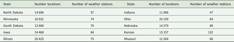
Ten major soybean-growing states (Fig. 1) were selected based on the larger production area to include diverse and extensive crop-growing environments. The subunits of the study area were counties of the respective states. The soil data were obtained from the Next Season System LLC under a special agreement. These data were created based on the Soil Survey Geographic Database (SSURGO) following methodology by Romero et al. (Reference Romero, Hoogenboom, Baigorria, Koo, Gijsman and Wood2012) in Decision Support System for Agrotechnology Transfer (DSSAT) format (Jones et al., Reference Jones, Hoogenboom, Porter, Boote, Batchelor, Hunt, Wilkens, Singh, Gijsman and Ritchie2003; Hoogenboom et al., Reference Hoogenboom, Porter, Boote, Shelia, Wilkens, Singh, White, Asseng, Lizaso, Moreno, Pavan, Ogoshi, Hunt, Tsuji, Jones, Usda-Ars and Boote2019), which describes the physical, chemical and hydraulic properties of stratified vertical layers of soil. Therefore, these soil input values carry valuable information to simulate root growth and development along with soil water balance and irrigation water needs. Soil water balance from the first day of the year to the start of crop simulation at planting serves as initial soil water for plant growth. Table 1 shows the number of locations used in the simulation. These locations represent the different soybean-growing areas.

Fig. 1. Soybean-producing states in the USA under study.
Table 1. Number of locations and weather stations for each state used for soybean simulation over a period of 1984–2010
Climate data and future climatic scenarios
Observed climate series
The Serially Completed Dataset (You et al., Reference You, Hubbard, Shulski, Svoboda and Hayes2015) for 30 years (1984–2010) for maximum temperature, minimum temperature and precipitation was gathered from High Plains Regional Climate Center (HPRCC) across weather stations of each state (Table 1). Solar radiation (daily insolation incident on a horizontal surface [MJ/m2/day]) data were obtained from the NASA-POWER agro-climatology dataset with a 1° × 1° resolution which was available starting only from July 1983. Therefore, the climate data from 1984 to 2010 (hereafter Observed Climate Series (BCS)) were used for crop simulation.
CMIP5 global climate models
This study uses eight different GCMs from CMIP5, which were selected to include models from different centres and had decadal as well as long-term future projections. Supplementary Table 1 lists the number of ensemble members for each model and their other characteristics which are derived from IPCC data distribution centre (https://www.ipcc-data.org/sim/gcm_monthly/AR5/Reference-Archive.html). CMIP5 includes coupled model decadal predictions for both the recent past and the future (Taylor et al., Reference Taylor, Stouffer and Meehl2012) as the output of decadal prediction experiment. The decadal1980 and decadal2005 experiment outputs were generated by initializing the experiment in the years 1980 and 2005 spanning a 30-year duration from 1981 to 2010 and 2006 to 2035, respectively. For each model, at least three ensembles from the decadal experiments were employed. Long-term projections based on two RCPs, RCP8.5 and RCP4.5, were included in this study. These projections span from the year 2006 to 2100, and even up to the year 2300 in the case of some models. However, only projections from 2006 to 2099 were considered in this research. Each model has at least one ensemble member for all variables under study.
Downscaling GCMs output
In this work, the GCM projection signal at each weather station was captured using the delta change approach of statistical downscaling. The signal was extracted as the delta for the near-surface monthly mean, maximum and minimum temperatures and as a ratio or factor for change in precipitation amount (Kraainjenbrink, Reference Kraaijenbrink2013), a monthly fraction for the number of wet days, and the standard deviation of maximum and minimum temperatures.
At first, the monthly mean across all of the ensembles of decadal1980 predictions of each model was calculated for the period of 1981–2010 for each variable (maximum temperature, minimum temperature, precipitation amount). Wet day's fraction for a particular month was calculated as the ratio of the number of wet days to the number of days in the month. A day with more than 1 mm precipitation in the model output was considered a wet day since the model predicts more wet days for a lower threshold of precipitation because of lower spatial resolution or due to drizzle problem (Polade et al., Reference Polade, Pierce, Cayan, Gershunov and Dettinger2014). Similar steps were followed to calculate the mean/or ratio of each variable using decadal2005 predictions and future climate scenarios forced by either RCP4.5 or RCP8.5 for the period 2006–2035. Subsequently, each ensemble of future climate projections forced by either RCP8.5 or RCP4.5 of the respective model was divided into nine decadal time scales (2010–2019, 2020–2029, 2030–2039, 2040–2049, 2050–2059, 2060–2069, 2070–2079, 2080–2089 and 2090–2099) and a monthly average of each decade for each parameter was calculated. Similar steps were followed to get the monthly standard deviations for maximum and minimum temperatures.
Calculation of systematic error (E) for each variable
The long-term future projections were based on greenhouse gas concentration as defined by RCPs, whereas decadal predictions were based on model runs initialized with actual atmospheric, oceanic and sea ice states along with external radiative forcing (Taylor et al., Reference Taylor, Stouffer and Meehl2012; Gaetani and Mohino, Reference Gaetani and Mohino2013). Therefore, the effect of initialization (as a systematic error) was needed to be calculated by taking the differences between decadal prediction and long-term future projections from the same model for a particular period (2006–2035) (Meehl and Teng, Reference Meehl and Teng2014). Systematic error was calculated as a difference of decadal 2005 prediction and future climatic scenarios forces by either RCP4.5 or RCP8.5 for the period of 2006–2035 for monthly mean maximum and minimum temperature. The ratio was calculated for change in precipitation amount (Kraainjenbrink, Reference Kraaijenbrink2013), a monthly fraction for the number of wet days, and standard deviation of maximum and minimum temperature.
Calculation of delta or factor change in each variable
The monthly delta change in maximum and minimum temperature was calculated for each ensemble of each model as differences between monthly mean of decadal1980 prediction for a span of 1981–2010 and each decade [nine decadal time scales (2010–2019, 2020–2029, 2030–2039, 2040–2049, 2050–2059, 2060–2069, 2070–2079, 2080–2089 and 2090–2099)] of each ensemble member of models for RCP4.5 or RCP8.5. Similarly, ratio was taken for other variables.
Calculation of error-corrected delta or factor
The delta or factor change and systematic error values calculated were then extracted from the native GCM grid-scale to the point or weather station level. Then, delta change and systematic error were used to derive corrected delta or factor change for each variable to neutralize the effect of initialization in decadal prediction. The error corrected delta for maximum and minimum temperature for each ensemble was computed by taking differences between delta change and respective systemic error. Similarly, the ratio was computed for other variables. The corrected factor for the monthly total precipitation was limited to the maximum value of three, which denotes the 300% increase in the monthly total precipitation in future compared to the decadal hindcast, which is likely in the dry season. Similarly, the corrected factor for wet day's fraction was limited within the range of 0.25–10 indicating that the number of wet days in future is 25% and 1000% lower and higher than the wet days in decadal hindcast.
Applying the mean and variability change to historical observed climate
AgMIP has provided protocols to generate probabilistic future climate series titled ‘Guide for Running AgMIP Climate Scenario Generation Tools with R’ (Hudson and Ruane, Reference Hudson, Ruane, Rosenzweig and Hillel2015). This procedure allows the imposition of mean and variability change signal from GCM output to observed climate to generate future climate series. It also considers the change in the number of rainy days in the future climate series (Ruane et al., Reference Ruane, Winter, McDermid, Hudson, Rosenzweig and Hillel2015). In this method, the expected future climate value is calculated based on the observed and expected distribution percentiles corresponding to the observed climate events (Rosenzweig et al., Reference Rosenzweig, Jones, Hatfield, Antle, Ruane, Boote, Thorburn, Valdivia, Porter, Janssen, Mutter, Rosenzweig and Hillel2015).
As the future climate signal was downscaled on the decadal basis, each downscaled signal [near-century (2010–2019, 2020–2029, 2030–2039), mid-century (2040–2049, 2050–2059, 2060–2069), late-century (2070–2079, 2080–2089, 2090–2099)] was applied to baseline observed climate series (BCS). Since each term contained three decades, the BCS was also divided into three periods (1984–1990, 1991–2000 and 2001–2010). The corrected delta and factor of the first decade of each term (2010–2019, 2040–2049, 2070–2079) were applied to first period (1984–1900) of BCS, second decade of each term (2020–2029, 2050–2059, 2080–2089) to second period (1991–2000) of BCS and third decade of each term (2030–2039, 2060–2069, 2090–2099) to third period (2001–2010) of BCS. The historical observed baseline in the procedure resembles one of the periods of the BCS to which delta and factor of a respective decade of each ensemble of each model were applied (Fig. 2).

Fig. 2. Flow chart to generate the future climate series using global climate models signal and observed climate series.
Crop simulation
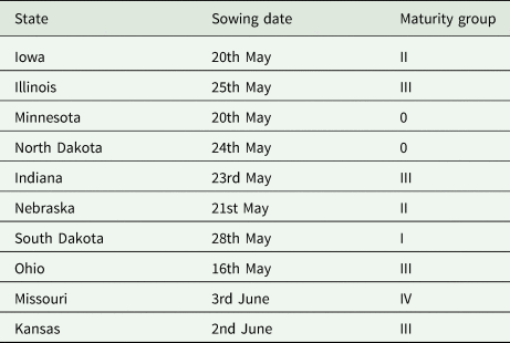
CROPGRO-Soybean, embedded under the DSSAT (Jones et al., Reference Jones, Hoogenboom, Porter, Boote, Batchelor, Hunt, Wilkens, Singh, Gijsman and Ritchie2003; Hoogenboom et al., Reference Hoogenboom, Porter, Boote, Shelia, Wilkens, Singh, White, Asseng, Lizaso, Moreno, Pavan, Ogoshi, Hunt, Tsuji, Jones, Usda-Ars and Boote2019) suite version 4.6 (Hoogenboom et al., Reference Hoogenboom, Jones, Wilkens, Porter, Boote, Hunt, Singh, Lizaso, White, Uryasev, Ogoshi, Koo, Shelia and Tsuji2015), was employed to simulate the soybean crop. Default genetic coefficients included in DSSAT for different maturity groups were used to simulate different soybean varieties. The soybean maturity group for each state (Table 2) was selected based on maps developed by Zhang et al. (Reference Zhang, Kyei-Boahen, Zhang, Zhang, Freeland, Watson and Liu2007). The information on active planting dates in each state was gleaned from the National Agricultural Statistics Service under the United States Department of Agriculture (USDA-NASS) based on the handbook ‘Field Crops Usual Planting and Harvesting Dates’ (USDA, 2010). The climate and soil regions homogenous map (Climate-Soil Simulation Unit Maps) for each state was obtained from Next Season System LLC.
Table 2. List of the most active planting dates of soybean
The simulation areas were selected based on the NASS maps of current cropping areas. The Geospatial Environmental Modeling (GEM; Baigorria and Romero, Reference Baigorria and Romero2007) software provided by Next Seasons Systems LLC was used to automate crop simulations. The state climate-soil unit map was overlaid on current soybean-growing area. For each location, the nearest weather station (Table 1) climate data were used for the simulation. The resulting map determined the density and region of crop simulation for each crop. The crop was simulated at each climate-soil unit using both observed (1984–2010) and future climate for three periods (2013–2039, 2043–2069, 2073–2099). Since 15 future climate series were generated under each RCP for each future period, there were 15 crop simulations of each crop at each climate-soil unit for the specified future period. Further, crop simulation runs were made separately under two water regime production systems (rainfed and irrigated) and two RCPs (RCP4.5 and RCP8.5). The climate from the nearest weather station of each soil unit was considered as weather input for crop models.
The carbon dioxide concentration was set at 400 ppm. The single planting date was envisaged for each state (Table 2) based on the most active planting date provided by USDA (2010). The plant population was set to 34 plants/m2 for both production systems, which is within the range of recommendation for optimum plant population in the Midwest, including northern parts of West North Central. For irrigated condition, water application was automated through sprinkler irrigation method when the simulated soil water was depleted below 75% of the total available water (i.e. 25% depletion below field capacity) in the soil layer of 30 cm depth. The highest level of irrigation water use efficiency (one) was considered for sprinkler irrigation method. The soybean crop did not get the additional supply of nitrogen throughout the growing season. The crops were set to be harvested at physiological maturity.
Analysis
The crop simulation outputs were summarized based on the production system (irrigated and rainfed), RCPs and the three future periods. Each future period had 27 years. Therefore, the crop simulation outputs at each location using individual series were averaged across the 27 years. Then, the output was further compiled by taking the mean of averaged values (27 years' average) at each location from 15 future series. Results were further summarized by taking mean across all the locations in each county under each state. The state average was calculated using the relative changes in the counties of each state. For the baseline period, crop simulation outputs at each location were averaged across the 27 years. The resulting averaged values were further summarized by taking the mean across all the locations in respective counties in each state (Fig. 3).

Fig. 3. Flow chart to summarize the crop simulation output from soil unit to state level.
The final output was conveyed as the relative percentage change (Eqn (1)) in each term [near-century (2013–2039), mid-century (2043–2069) and end-century (2073–2099)] compared to observed simulation at the county level. Each production system's (rainfed and irrigated) baseline simulation was used to calculate the relative percentage change in variables under the respective production system in the future.

where, Simfuture = simulated value for future period for a county and Simobs = simulated value for baseline period for a county.
Similarly, water productivity was computed under both irrigated and rainfed conditions. Usually, water productivity is calculated in terms of either evapotranspiration or irrigated water applied to the field. Water productivity was estimated based on the total seasonal evapotranspiration (Bezerra, Reference Bezerra and Lee2012) following Eqn (2).

where, WPET, water productivity in terms of crop evapotranspiration; GY, crop grain yield (kg/ha); ET, seasonal evapotranspiration (mm/ha).
Further, future water requirement for irrigation in each state was computed based on the change in water demand, baseline simulated water requirement and the total area of cultivated land for each crop. The water requirement was expressed in terms of millions m3 for each state. Finally, maps were developed for a number of variables including seasonal length, grain yield, evapotranspiration and water productivity in future period for effective visual comparison. The values depicted in the map represent relative changes in the simulated variables at state levels. The maps for baseline simulation were based on actual values for both irrigated and rainfed production systems whereas the relative percentage change was used to represent the change in crop growth and other parameters in the future period (2013–2039, 2043–2069, 2073–2099) compared to baseline simulation. The counties with no simulation were shown in white colour on each map.
Results
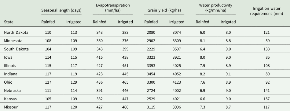
Soybean simulations under future periods were presented as the relative percentage change in various parameters compared to the observed simulation. The results were compared across two RCPs and three future periods under both irrigated and rainfed conditions. Since this study focused on water requirements and crop grain yield, selective response variables including seasonal length, seasonal evapotranspiration, additional irrigation water requirements and crop grain yield were evaluated and discussed. Furthermore, each variable was presented through maps to make a visual comparison. The observed climatic variables and simulated soybean parameters during the soybean-growing season are presented in Tables 3 and 4.
Table 3. Observed seasonal average of the climatic parameters over a period of 1984–2010 under rainfed and irrigated soybean
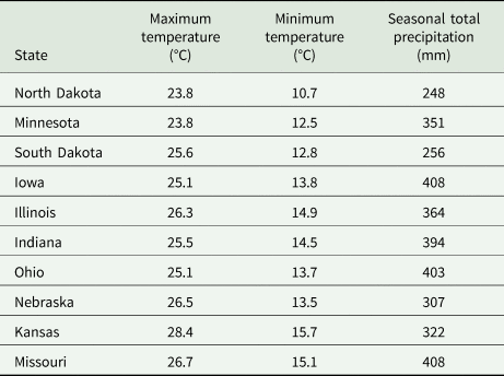
Table 4. Simulated observed parameters of soybean over a period of 1984–2010
Relative change in climatic variables
Since the relative changes in climatic variables under rainfed and irrigated conditions are identical, changes under rainfed conditions are used to analyse the patterns of change in temperature and precipitation. Under RCP8.5, the positive relative changes in maximum and minimum temperature are greater than under RCP4.5, and the magnitude of these changes increases as time progresses. In addition, relative changes in maximum temperature are greater than minimum temperature across all time periods, states and RCPs (Figs 4(a) and (b)). The average increase in relative changes in maximum and minimum temperature across all the states is up to 10.2 (2.6°C) and 19.3 (2.6°C) under RCP4.5 and 19.8 (5.1°C) and 36.7 (4.9°C) under RCP8.5, respectively, at end-century period. The relative changes are more pronounced in northern states than southern states (Fig. 5 (a) and 5 (b)); however, the actual changes in seasonal temperature are expected to vary little. North Dakota is likely to experience highest relative changes in maximum and minimum temperature compared to other states under both scenarios along with maximum average seasonal maximum and minimum temperature changes of 5.2°C.

Fig. 4. Change in seasonal (a) maximum temperature (°C), (b) minimum temperature (°C) and (c) total precipitation (mm) compared to observed (1984–2010) in rainfed condition.
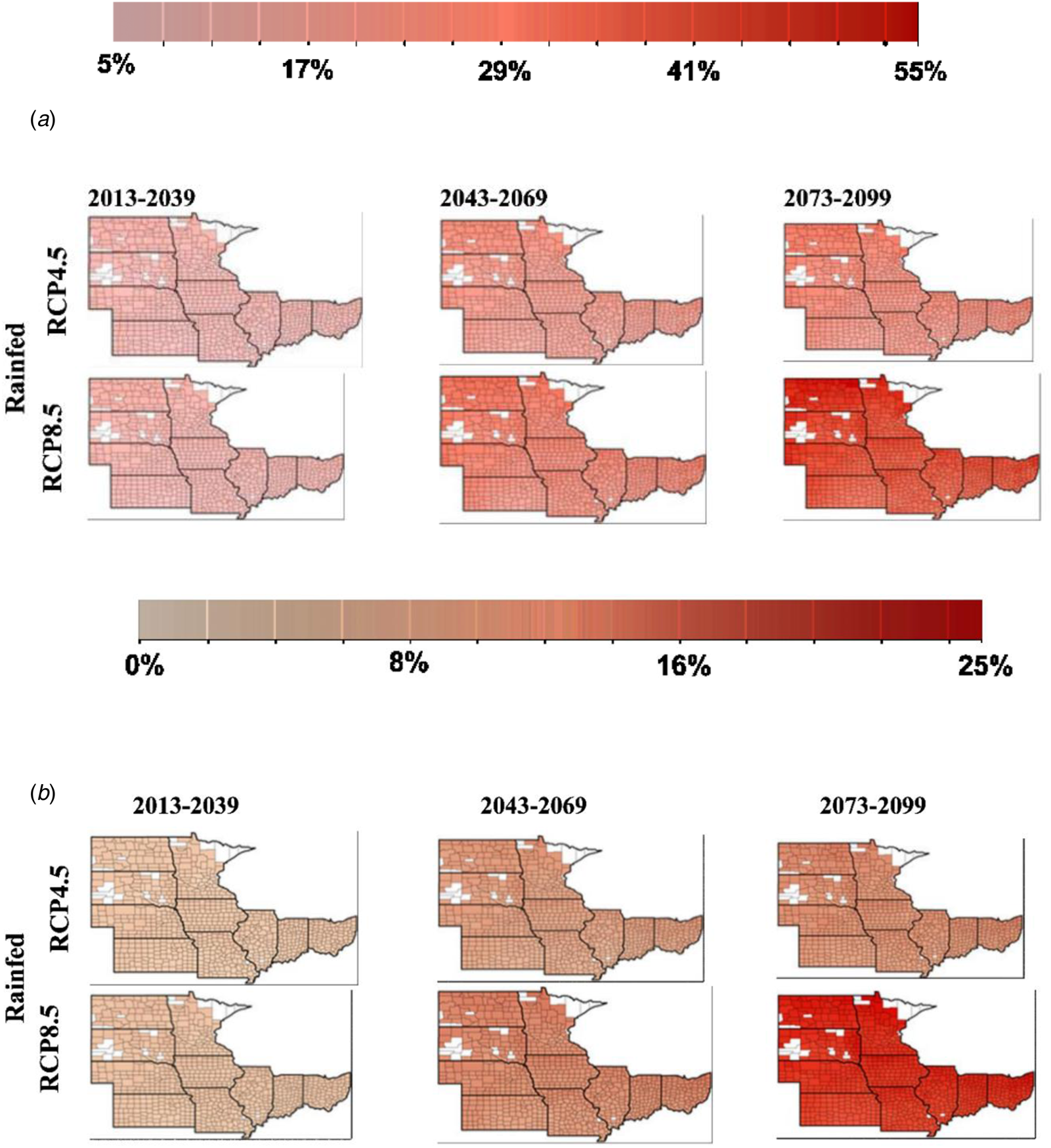
Fig. 5. Change in seasonal (a) maximum temperature, and (b) minimum temperature (%) in rainfed condition under RCP4.5 and RCP8.5.
Total seasonal precipitation is projected to follow a similar trend to temperature, but the relative changes are negative, implying a drop in seasonal precipitation across all scenarios and periods. As years progress, the changes are likely to become more pronounced. The northern states are likely to experience higher relative change in seasonal precipitation amount compared to southern states. The highest change in seasonal precipitation is expected up to 25 mm in Nebraska under RCP4.5 and 45 mm in Iowa under RCP8.5 at end-century period (Fig. 4(c)).
Relative change in seasonal length
The soybean life cycle is expected to be shortened in the future under both RCPs. The relative changes increase with advancement towards the end of the century under both rainfed and irrigated conditions. The impact on the simulated seasonal length is expected to be higher under RCP8.5 than RCP4.5. Under rainfed conditions, the reductions are up to 8.7 days (Minnesota and North Dakota) under RCP4.5 and up to 14 days (North Dakota) under RCP8.5. Similarly, under irrigated conditions, life cycle will be reduced up to 8.1 and 11.7 days (Minnesota) under RCP4.5 and RCP8.5 at the end of the century. For every time slice, the predicted changes are greater under the water-limited growing environment than in the irrigated condition. In North Dakota and Minnesota, soybean simulated with maturity group 0 is expected to experience higher reduction. Lower change in predicted seasonal length was found in southern states simulated with higher maturity groups. Contrast to the trend obtained for other states, the result shows positive predictive changes in seasonal length in the end-century period under RCP8.5 in most of the regions of Kansas and southern parts of Missouri and Illinois. However, based on county averages, only Kansas under RCP8.5, in both rainfed and irrigated conditions, is predicted to have 2 days longer life cycle by the end-century period. It is also evident that the reduction in soybean life cycle is expected to be higher in northern parts within each state, especially in Iowa, Illinois, Indiana and Ohio for the mid- and end-century periods (Fig. 6).
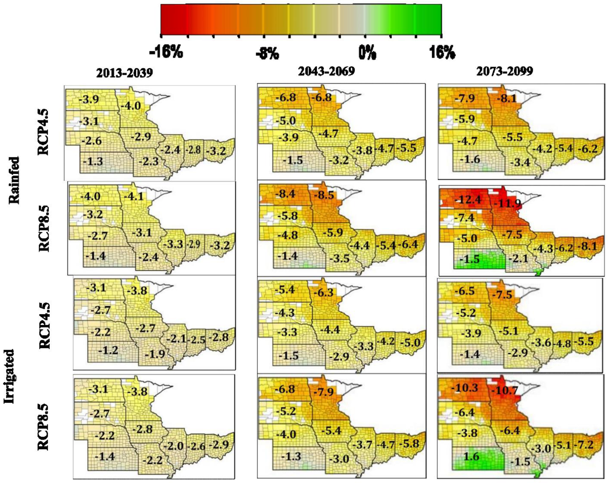
Fig. 6. Relative change in seasonal length (%) in rainfed and irrigated conditions under RCP4.5 and RCP8.5.
Relative change in evapotranspiration
The change in evapotranspiration shows a different trend in three time slices under rainfed and irrigated conditions. In rainfed condition, under both RCPs, evapotranspiration is predicted to decrease in all states at the first time slice. In other time slices, only North Dakota, Minnesota, South Dakota and Nebraska under both RCPs, as well as Indiana under RCP4.5, will experience reduced evapotranspiration. As the century progresses, the other states (Iowa, Illinois, Indiana, Kansas and Missouri) are expected to see an increase in evapotranspiration. Under irrigated conditions, excluding Minnesota at initial time slice, evapotranspiration loss of water will grow and become more intense as the century advanced under both RCPs (Fig. 7). Moreover, change in evapotranspiration will be more in Illinois (47.3 mm) followed by Kansas (46.9 mm) and Missouri (46.0 mm) under RCP8.5 and Kansas (18.7 mm), Illinois (17.5 mm) and Missouri (17.1 mm) (3.9) under RCP4.5 at the late century compared to the early-century period. Further, the result also shows the trend that the southern states are expected to experience the higher change in evapotranspiration demand than the northern states (Fig. 7). In both production systems, the change in evapotranspiration was found to be greater in most situations under RCP8.5 than under RCP4.5 (Fig. 7).
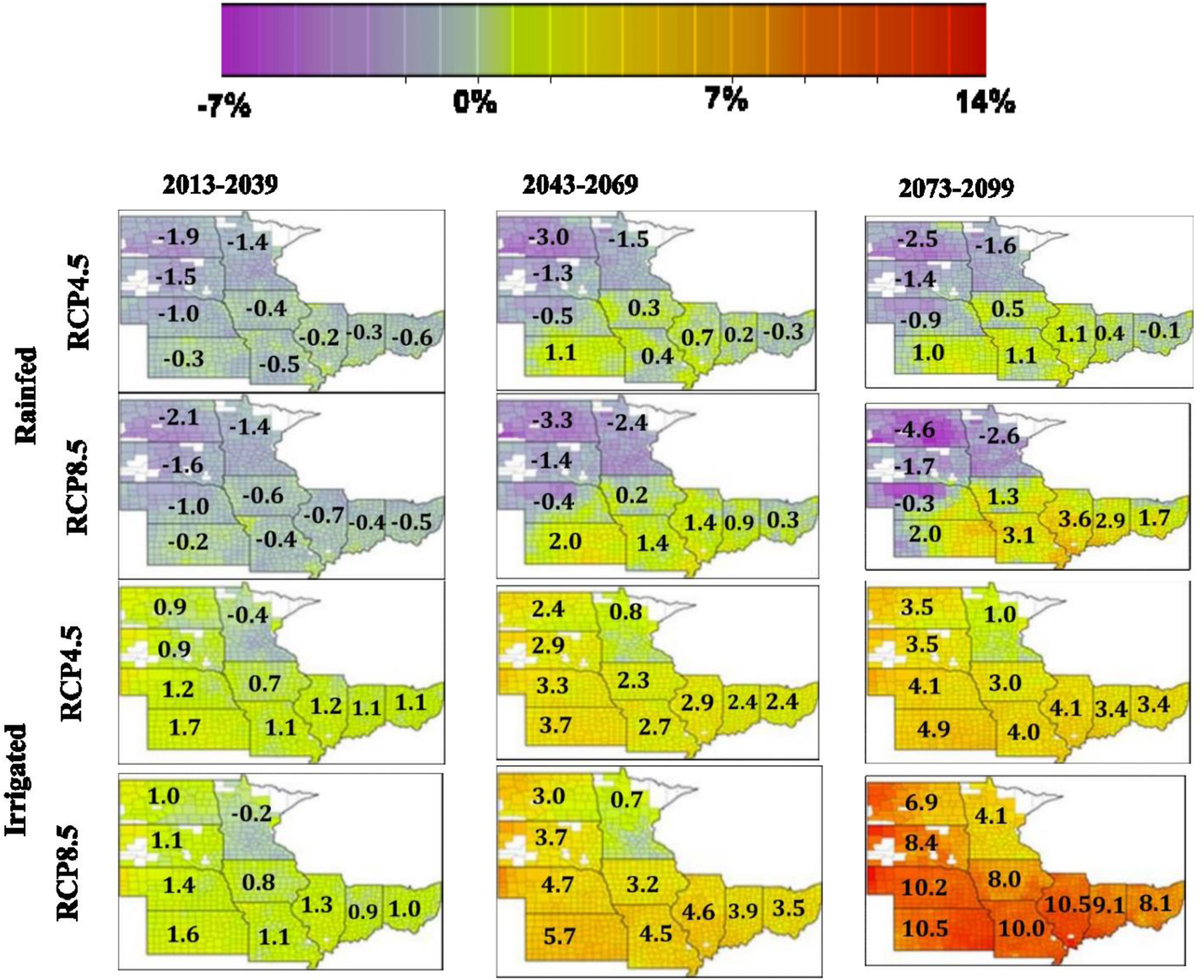
Fig. 7. Relative change in evapotranspiration (%) in rainfed and irrigated conditions under RCP4.5 and RCP8.5.
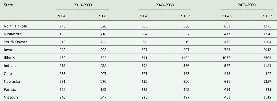
Additional water requirement
The additional water requirement was calculated for the state as if all the area would be brought under the irrigated condition. The precipitation amount is likely to change under both scenarios in future (Fig. 8). Under both representative concentration routes, soybean production will require more extra water in the future (Table 5). The water demand is higher under RCP8.5 than under RCP4.5. The water demand under the two RCPs will be wider in the third phase compared to the first and the second phase (Table 5). As the 21st century progresses, the requirement for water will increase for soybean production in all states (Fig. 9). On average, over ten states, the water demand under RCP8.5 will be 23.8, 179.9 and 765.8 million m3 higher than RCP4.5 in three time slices, respectively.

Fig. 8. Change in total seasonal precipitation (%) in under RCP4.5 and RCP8.5.
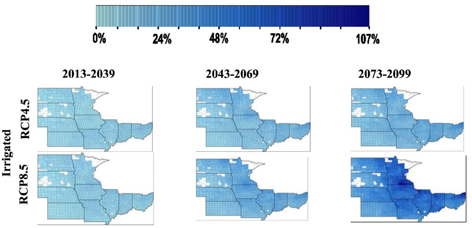
Fig. 9. Relative change in irrigation volume (%) in irrigated condition under RCP4.5 and RCP8.5.
Table 5. Additional water requirement (millions m3) per cropping season for each state
Relative change in grain yield
The rainfed soybean was found to have a negative response in crop yield compared to the irrigated condition across both RCPs and time slices (Fig. 10). The predicted decrease in grain yield is likely to be more intensified with the advancement towards the end-century period. Similarly, the magnitude of the reduction is expected to be higher in RCP8.5 compared to RCP4.5 under each production system (Fig. 10). Under rainfed conditions, except for North Dakota and Minnesota, all states are likely to reduce the grain yield in all three time slices. Under rainfed conditions, the average loss across the ten states under RCP8.5 at the end-century period will be around 871 kg/ha (Supplementary Table 2). Minnesota will not lose yield at the first time slice under both RCPs under rainfed conditions. It will also be benefitted under the irrigated condition, except under RCP8.5. In North Dakota, grain yield is likely to increase in both rainfed and irrigated conditions except in the end-century period under RCP8.5. South Dakota will only experience a decrease in yield under irrigated condition with the RCP8.5 scenario at the mid- and end-century periods. The remaining states are anticipated to have a drop in grain yields, which will intensify as the century progresses (Fig. 10). Kansas, Missouri, Nebraska and Illinois are among the states likely to lose greater grain yields in the future. Kansas is predicted to have the largest decrease in yield (1126 kg/ha) under RCP8.5 by the end of the century, followed by Nebraska (760 kg/ha), Missouri (679 kg/ha) and Illinois (644 kg/ha) under irrigated condition (Fig. 10). However, the ranking based on the decrease in simulated yield will be Illinois (1154 kg/ha) followed by Nebraska and Kansas (1062 kg/ha) and Missouri (1059 kg/ha) under rainfed conditions and RCP8.5 scenario (Supplementary Table 2). Under irrigated conditions, the North Dakota might witness an increase in grain yield up to 492 kg/ha under the second time slice with both RCPs and under the third time slice with RCP4.5.

Fig. 10. Relative change in grain yield (%) in rainfed and irrigated conditions under RCP4.5 and RCP8.5.
Relative change in water productivity
Water productivity is considered as the ratio of grain yield to evapotranspiration. Hence, higher water productivity represents a higher grain yield per unit loss of water through evapotranspiration. The rainfed soybean is likely to experience a higher decrease in water productivity in each term when compared to the irrigated soybean. It is also evident that water productivity is likely to increase in some northern parts (Fig. 11) of the study area. Under the irrigated condition, North Dakota, Minnesota (except end-century under RCP8.5) and South Dakota (in early-century) are found to experience positive relative overall changes, whereas the rainfed soybean might experience an increase in water productivity only in North Dakota (except in the end-century under RCP8.5) and Minnesota (only in the early-century) (Supplementary Table 3). Kansas is likely to have the lowest water productivity. Other states with lower water productivity are Nebraska, Missouri and Illinois. The decrease in water productivity is higher under RCP8.5 than under RCP4.5, especially in the mid- and end-century periods. The predictive reduction was found to be more than doubled in the end-century period under RCP8.5 when compared to RCP4.5. The changes in water productivity are expected to be higher in the southern parts than in the northern parts of most of the states (Fig. 11).

Fig. 11. Relative change in water productivity (%) in rainfed and irrigated conditions under RCP4.5 and RCP8.5.
Discussion
Heat and water stress are growing climatic threats to soybean production (Jin et al., Reference Jin, Zhuang, Wang, Archontoulis, Zobel and Kotamarthi2017). It is estimated that about one-third variation in soybean yield in the USA could be attributed to the precipitation and temperature variations (Vogel et al., Reference Vogel, Donat, Alexander, Meinshausen, Ray, Karoly, Meinshausen and Frieler2019) and average soybean yield gain in the USA was suppressed by 30% than that realized yield gain by producers over 1994–2013 due to the combined precipitation and temperature variations, worth US$11 billion (Mourtzinis et al., Reference Mourtzinis, Specht, Lindsey, Wiebold, Ross, Nafziger, Kandel, Mueller, Devillez, Arriaga and Conley2015). The information-intensive technological development may help to reduce the harmful consequences of climate change on soybean production (Burchfield et al., Reference Burchfield, Matthews-Pennanen, Schoof and Lant2020), demanding a range of climate change-related impact studies on soybean. Many impact studies are based on change in mean (Mearns et al., Reference Mearns, Rosenzweig and Goldberg1997; Anapalli et al., Reference Anapalli, Fisher, Reddy, Pettigrew, Sui and Ahuja2016; Schleussner et al., Reference Schleussner, Deryng, Müller, Elliott, Saeed, Folberth, Liu, Wang, Pugh, Thiery, Seneviratne and Rogelj2018); however, changes in mean are not only accountable for crop performance but variation in climatic parameters on temporal (Gornall et al., Reference Gornall, Betts, Burke, Clark, Camp, Willett and Wiltshire2010; Strzepek and Boehlert, Reference Strzepek and Boehlert2010; Leng et al., Reference Leng, Zhang, Huang, Asrar and Leung2016; Shortridge, Reference Shortridge2019, Odey et al., Reference Odey, Adelodun, Cho, Lee, Adeyemi and Choi2022) and spatial scale (White et al., Reference White, Hoogenboom, Kimball and Wall2011; Bandara et al., Reference Bandara, Weerasooriya, Murillo-Williams, White, Collins, Bell and Esker2020). So, crop–environment relationships are better understood when they are studied over a larger area, for longer periods of time and with mutimodel approach for using GCMs to reflect a broader range of possible future development possibilities (Woznicki et al., Reference Woznicki, Nejadhashemi and Parsinejad2015). Therefore, we studied the soybean performance under three time scales, two RCPs-based scenarios and two water regime conditions over the ten major soybean-growing states of the USA. A total of 160 964 locations were used in simulations using CROPGRO-Soybean for evaluating the seasonal length, evapotranspiration, water demand, yield and water productivity.
In soybean, photoperiod primarily stimulates the transition from vegetative to reproductive phase (Borthwick and Parker, Reference Borthwick and Parker1938). Similarly, the temperature determines the rate at which a crop develops (Hatfield and Prueger, Reference Hatfield and Prueger2015). Besides temperature, water stress is also responsible for determining the soybean lifecycle. The water stress during flower induction and flowering results in shorter flowering period (Sionit and Kramer, Reference Sionit and Kramer1977). Based on this study, a shorter soybean life cycle could be expected as the 21st century progressed with increased temperatures and decreased precipitation. Under both rainfed and irrigated environments, the relative change in life cycle length under RCP8.5 is greater than under RCP4.5 under each time slice because of comparatively higher temperature and reduced precipitation under RCP8.5. Further, a shortened life cycle in a water-stressed rainfed condition might be related to water stress compared to irrigation condition. Bao et al. (Reference Bao, Hoogenboom, McClendon and Urich2015) also predicted a decrease in soybean life cycle by 1.8 and 2.3 days by 2025 and 2050, respectively, under water-limited and irrigated condition in the southeastern USA. The northern states like North Dakota and Minnesota are expected to experience up to 14 and 13 days under rain fed and 11.6 and 11.7 days average reduction in life cycle under irrigated conditions with RCP8.5 scenarios, respectively, at the end of the century. Cultivars with different maturity groups might be responsible for this regional heterogeneity. Earlier maturity cultivars, which are modelled for northern states, are less responsive to day duration (Boote et al., Reference Boote, Kropff and Bindraban2001). Temperature and water stress are therefore more responsible for crop growth and development. Later maturity groups, on the other hand, are more sensitive to day duration, which may have resulted in a smaller relative shift in predicted crop seasonal length in southern states with higher maturity groups. Furthermore, as observed by Choi et al. (Reference Choi, Ban, Seo, Lee and Lee2016) in South Korea for Sinpaldalkong and Daewonkong cultivars under field conditions, the supra-optimum temperature may have slowed the reproductive phase to extend the seasonal duration in portions of Kansas and southern parts of Missouri and Illinois.
Evapotranspiration is the total of soil water evaporation and transpiration by plant surfaces (Liu and Basso, Reference Liu and Basso2020; Varmaghani et al., Reference Varmaghani, Eichinger and Prueger2021). Total evapotranspiration from soybean production will rise as the 21st century advanced in irrigated conditions under both RCPs with increased temperature. Northern states are likely to have lower seasonal evapotranspiration, which could be attributed to the shorter expected life cycle of soybean and decreased precipitation. Precipitation and length of the season are expected to drop less in southern states like Missouri and Kansas. Because of this, the volume of water evapotranspiring was likely to be larger at the end-century period under RCP8.5. The higher relative changes under RCP8.5 as compared to RCP4.5 might be attributable to a greater increase in temperature and a drop in seasonal precipitation. Irrigated fields are likely to lose more water under expected future climate compared to water constrained fields.
Given the predicted temperature and precipitation patterns in the various parts of the country, the quantity of irrigation water may vary significantly. As the 21st century progresses, irrigation water demand will increase soybean production in all states. On average, over ten states, the water demand under RCP8.5 will be 23.8, 179.9 and 765.8 millions m3 per season higher than RCP4.5 in three time slices, respectively. A greater rate of evapotranspiration and lower anticipated seasonal precipitation might be responsible for this trend.
With management practices (planting density, spacing, sowing dates, fertilizer doses) specified for this study, yield losses will be substantially higher by the end of the century, averaging across ten states 310 and 1154 kg/ha under RCP4.5 and RCP8.5 for the end-of-century period under rainfed conditions, respectively. Due to limited temperature-driven growth in North Dakota and Minnesota at present, the elevated temperatures in future might help for proper early growth and development of the crops, which might lead to an increase in the yield. In other states, yield loss will be higher as we further advance into the future. The yield loss in RCP8.5 is expected to be greater than under RCP4.5 in areas having negative consequences of future climate; increased temperature, lowered precipitation and their variation over time. The combined effects of increased heat and water stress may have resulted in a greater relative drop in grain production under rainfed conditions compared to irrigated conditions. Ohashi et al. (Reference Ohashi, Nakayama, Saneoka and Fujita2006) also reported a 30% lower biomass yield from water stressed soybean when compared to the biomass yield from well-watered soybean.
Water productivity will follow a similar trajectory in the future as grain yield. Comparatively, higher temperatures under RCP8.5 may have resulted in decreased water productivity compared to RCP4.5, and the same rationale may account for higher relative changes in southern sections of most states than northern parts. In North Dakota and Minnesota, increase in water productivity could be attributed to the temperature increment impact on the grain yield. The greater decline in grain yield under rainfed conditions might have resulted in lower water productivity. Kang et al. (Reference Kang, Khan and Ma2009) also reported that soil evaporation and plant transpiration would be affected due to climate change's impact on soil water balance, which could shorten crop seasonal length impacting water productivity.
In the USA, irrigation has been regarded as a viable strategy to lessen the impact of climatic unpredictability on agricultural production (Kukal and Irmak, Reference Kukal and Irmak2020). From this study, the increasing irrigation water demand indicates the anticipated precipitation will not be sufficient to support the soybean production in study areas in the future. Moreover, irrigation can be taken as possible coping strategies against future climate change. However, as diverse sectors strive to reduce the threat of water shortages in the face of rising climatic variation, water resource management will become increasingly more essential (Cherkauer et al., Reference Cherkauer, Bowling, Byun, Chaubey, Chin, Ficklin, Hamlet, Kines, Lee, Neupane, Pignotti, Rahman, Singh, Femeena and Williamson2021). In addition, the cost of production is likely to increase with additional water removal requirement (Fischer et al., Reference Fischer, Tubiello, van Velthuizen and Wiberg2007). This study shows slight shift in soybean production zone towards north. Cho and McCarl (Reference Cho and McCarl2017) also suggested a shift in crop production zones in the USA in response to change in temperature and precipitation for the 1970–2010 period. They also projected the majority of the crops to shift towards north and east in the future under RCP4.5 and RCP8.5 pathways.
There were noticeable changes in climate in the USA after the baseline period (1984–2010) considered in this study. In recent years (2010–2019), weather and climate-related disasters with at least $1 billion in damage costs have increased in the USA, with drought being one of the causes of significant disasters (Smith, Reference Smith2020). Moreover, the recent normal years (2091–2020) were warmer than the years in preceding decades, and the rate of temperature change is not uniform across the USA (Lindsey, Reference Lindsey2021). The years 2012 and 2016 were among the warmest years across the USA (EPA, 2022a). Similarly, wet and dry patterns have changed in different parts of the contiguous USA (Lindsey, Reference Lindsey2021). The drought in 2012 hit about 90% of soybean production areas till late July, the cause by 2952–2690 kg per hectare and a 113–104 billion reduction in soybean productivity and production, respectively, in the USA (Rippey, Reference Rippey2015). The mid-western region experienced significant soybean yield loss and which soared the global soybean price (Zhang et al., Reference Zhang, Zang, Li, Ma and Liu2018). This picture clearly shows that the future climate will pose a noticeable threat to soybean production in the USA. In this backdrop, the current study will help track the soybean yield in relation to the future climate.
Limitation of study
This study was carried out with a set of management techniques such as single planting date and a set of row spacing. Various management methods need to be investigated to determine the best adaption strategies for diverse soybean-producing zones. Strategies such as different durational varieties (Meng et al., Reference Meng, Chen, Lobell, Cui, Zhang, Yang and Zhang2016), shift in planting dates (Kumar et al., Reference Kumar, Pandey and Kumar2008; Bowling et al., Reference Bowling, Cherkauer, Lee, Beckerman, Brouder, Buzan, Doering, Dukes, Ebner, Frankenberger, Gramig, Kladivko and Volenec2020), crop rotation (Marini et al., Reference Marini, St-Martin, Vico, Baldoni, Berti, Blecharczyk, Malecka-Jankowiak, Morari, Sawinska and Bommarco2020), tillage practices (Liu and Basso, Reference Liu and Basso2020) and fertilizer use (Manna et al., Reference Manna, Bhattacharyya, Adhya, Singh, Wanjari, Ramana, Tripathi, Singh, Reddy, Subba Rao, Sisodia, Dongre, Jha, Neogi, Roy, Rao, Sawarkar and Rao2013; Afroz et al., Reference Afroz, Li, Muhammed, Anandhi and Chen2021) are being adopted in various regions of the world needs to be explored as adaptation strategies to climate change. The atmospheric carbon dioxide level was kept constant during simulation runs, despite the fact that CO2 levels are predicted to have a significant influence, particularly on C3 crops (Bernacchi et al., Reference Bernacchi, Kimball, Quarles, Long and Ort2007; Jin et al., Reference Jin, Zhuang, Wang, Archontoulis, Zobel and Kotamarthi2017). Moreover, the simulation did not take into account insect and disease dynamics. However, the changing temperature will alter the insect population (Kollberg et al., Reference Kollberg, Bylund, Jonsson, Schmidt, Gershenzon and Björkman2015), growth rate (Kiritani, Reference Kiritani2013), diseases appearance and severity (Bebber et al., Reference Bebber, Ramotowski and Gurr2013) and thereby their impact on the crops. Therefore, it is also necessary to take into account the indirect effects of insects and diseases (Gornall et al., Reference Gornall, Betts, Burke, Clark, Camp, Willett and Wiltshire2010; Raza et al., Reference Raza, Khan, Arshad, Sagheer, Sattar, Shafi, ul Haq, Ali, Aslam, Mushtaq, Ishfaq, Sabir and Sattar2015; Taylor et al., Reference Taylor, Herms, Cardina and Moore2018; Skendžić et al., Reference Skendžić, Zovko, Živković, Lešić and Lemić2021). Therefore, the use of the sophisticated model which considers the insect pest dynamics will help further to reach in valid conclusion. Climate change implications on global agricultural production cannot be reliably predicted because of the uncertainty of how high CO2 impacts crop physiology and productivity (Gornall et al., Reference Gornall, Betts, Burke, Clark, Camp, Willett and Wiltshire2010, Gray et al., Reference Gray, Dermody, Klein, Locke, McGrath, Paul, Rosenthal, Ruiz-Vera, Siebers, Strellner, Ainsworth, Bernacchi, Long, Ort and Leakey2016, Jin et al., Reference Jin, Zhuang, Wang, Archontoulis, Zobel and Kotamarthi2017), high variability in enclosed chambers and free-air carbon dioxide enrichment studies (Long et al., Reference Long, Ainsworth, Leakey, Nösberger and Ort2006), large regional differences in crop responses to CO2 (McGrath and Lobell, Reference McGrath and Lobell2013) and uncertainty in potential impact of weed species on crops (Ziska et al., Reference Ziska, Reeves and Blank2005; Hatfield et al., Reference Hatfield, Boote, Kimball, Ziska, Izaurralde, Ort, Thomson and Wolfe2011; Vilà et al., Reference Vilà, Beaury, Blumenthal, Bradley, Early, Laginhas, Trillo, Dukes, Sorte and Ibáñez2021). So, the biological plausibility of estimates should be strengthened by a more thorough various model intercomparison (White et al., Reference White, Hoogenboom, Kimball and Wall2011) in diverse environmental conditions. Moreover, the advancement in the breeding programme to ensure yield stability under stress conditions determines the impact of climate change on soybean production (Valliyodan et al., Reference Valliyodan, Ye, Song, Murphy, Shannon and Nguyen2017).
Conclusion
The soybean yield is expected to decline more under rainfed than irrigated conditions in most soybean-growing areas under study, which will harm farmers' resource use efficiency and profitability as the yield is already lower under rainfed than irrigated conditions. Supplemental irrigation water does not seem to optimize crop yield and water productivity; however, it could help to minimize the negative impact of future climate on crop performance, while marginal economic irrigation could become a concern in the future. Moreover, northern states under study are expected to enhance yield or have less impact on the future climate and could be key production zones for soybean production in the future, considering climate change as the principal factor. Furthermore, the greater impact on soybean under ‘business as usual’ scenarios signifies the necessity for stringent mitigation and adaptation policies.
Supplementary material
The supplementary material for this article can be found at https://doi.org/10.1017/S0021859623000011.
Acknowledgements
The authors would like to thank all the helping hands from the School of Natural Resources and the University of Nebraska-Lincoln. The authors would also like to acknowledge Dr Tala Awada from the School of Natural Resources and Dr Christopher Neale from Water for Food Institute for extra funding support for research, and Dr Consuelo C. Romero from Next Season Systems for providing research data and software. The authors also thank Nepal Agriculture Research Council for providing study leave for a period of 3 years.
Author contributions
A. P. Timilsina and G. A. Baigorria conceived and designed study. A. P. Timilsina conducted data gathering, analyses and wrote the article. D. Wilhite, M. Shulski and D. Heeren were responsible for supervision of graduate students and helped in improving the manuscript. C. Romero prepared the soil data file in DSSAT format. C. Fensterseifer gathered crop production data and helped in analyses.
Financial support
The funding support was provided by Dr Christopher Neale from Water for Food Institute, Lincoln, Nebraska.
Conflict of interest
None.
Ethical standards
Not applicable.


 Open access