


1. Introduction
Understanding the growth mechanism of surface water waves by the action of wind remains a long-standing problem in fluid mechanics and physical oceanography (Sullivan & McWilliams Reference Sullivan and McWilliams2010; Pizzo, Deike & Ayet Reference Pizzo, Deike and Ayet2021). Modern studies began with Jeffreys (Reference Jeffreys1925), who considered the work done by the pressure difference between the windward and leeward sides of the waves through a separated airflow: the ‘sheltering mechanism’. Lock (Reference Lock1954) studied the stability of a steady laminar stream of air over a surface of water at rest. His analysis is comparable to the stability of a Blasius boundary layer and yielded critical wind speeds in the range 1–3 m s $^{-1}$. Shortly after, Phillips (Reference Phillips1957) and Miles (Reference Miles1957) contributed to the problem, with Phillips (Reference Phillips1957) proposing a mechanism based on the resonant forcing of the waves by turbulent pressure fluctuations, and Miles (Reference Miles1957) proposing an inviscid instability caused by the coupling of the airflow shear with the water wave. Decades later, Belcher & Hunt (Reference Belcher and Hunt1993) coupled the idea of Jeffreys (Reference Jeffreys1925) sheltering theory to a turbulent airflow, giving the ‘non-separated sheltering mechanism’. A recent summary of these mechanisms and their history can be found in Pizzo et al. (Reference Pizzo, Deike and Ayet2021).
A conspicuous feature of the theory of Miles (Reference Miles1957) was the presence of a rapid change in flow behaviour at a critical layer height, the location where the wind speed matches the wave phase speed. Support for the critical layer mechanism of Miles (Reference Miles1957) has been found over the open ocean by Hristov, Miller & Friehe (Reference Hristov, Miller and Friehe2003), for wave ages  $c/u_*$ between 16 and 40 (also known as ‘intermediate’ to ‘fast’ waves; Belcher & Hunt Reference Belcher and Hunt1998), with a vertical array of anemometers indicating the presence of a critical layer that was largely in agreement with the theory (see also Grare, Lenain & Melville Reference Grare, Lenain and Melville2013). However, uncertainty with respect to wind-wave growth mechanisms still exists due to a number of difficulties, chief among them, the difficulty associated with conducting precise measurements near the wavy air–water interface (Sullivan & McWilliams Reference Sullivan and McWilliams2010).
We overcome this difficulty largely through the use of combined particle image velocimetry (PIV) and laser induced fluorescence (LIF) techniques, that allow for a high-resolution quantification of the two-dimensional airflow over growing wind-generated waves in a series of laboratory experiments (Buckley & Veron Reference Buckley and Veron2016, Reference Buckley and Veron2017). The results from one such experiment are examined here to quantify the role of the critical layer mechanism in a field of young, growing wind waves. This evidence consists essentially of providing a comparison between the experimental results and linear stability theory. It utilises a new diagnostic formulated from linear stability theory to assess the growth rate of the wind-wave instability directly from the laboratory observations. We demonstrate that the critical layer mechanism accounts for the total expected energy growth, and conclude that this mechanism can be an active and significant contribution to wind-wave growth in young seas. Indeed, the structure of the airflow, and the growth of the surface wave field in this laboratory experiment, can be captured largely by the original theory of Miles (Reference Miles1957), complete with its numerous simplifying assumptions.
The paper is organised as follows. We first outline the linear stability problem that forms the basis of formulating the growth diagnostic, then in § 3 we include a description of the results of the laboratory experiment, a comparison between experiment and linear theory, a quantification of the experimental growth rates, and a discussion. A summary and conclusions are presented in the final section.
2. Formulating a critical layer wave growth diagnostic
In this section, we derive a formula for the quantification of wind-wave energy growth based on linear stability theory. This follows the original analysis method of Miles (Reference Miles1957), which has been used subsequently by many others (e.g. Young & Wolfe Reference Young and Wolfe2014). In doing so, we linearise the equations of motion for perturbations to an incompressible inviscid two-dimensional flow, neglecting surface tension, about the background equilibrium described by the profiles  $U(z)$ and
  $\bar {\rho }(z)$. These can be written as
 \begin{gather} {\rm i}k\hat{u} + \hat{w}' = 0 , \end{gather}
 \begin{gather}\bar{\rho} ({\rm i}k(U-c)\hat{u} +\hat{w}U') ={-}{\rm i}k\hat{p} , \end{gather}
 \begin{gather}\bar{\rho} [{\rm i}k(U-c)\hat{w}] ={-}\hat{p}' - \hat{\rho} g , \end{gather}
 \begin{gather}{\rm i}k(U-c)\hat{\rho} + \hat{w} \bar{\rho}'= 0 . \end{gather}
Here, we have taken solutions to be of the normal mode form,  $w(x,z,t) = \mathrm {Re}\{ \hat {w}(z)\, {\rm e}^{{\rm i}k(x-ct)} \}$, for the vertical velocity perturbation
  $w$, as well as for the horizontal velocity perturbation
  $u$, the density perturbation
  $\rho$, and the pressure
  $p$. In addition,
  $k$ represents the horizontal wavenumber,
  $c$ the complex wave phase speed, and
  $g$ the gravitational acceleration, and primes denote differentiation with respect to
  $z$.
$z$.
The linear stability problem is written compactly in terms of the vertical velocity eigenfunction  $\hat {w}(z)$ and the complex wave speed eigenvalue
  $c$, with the following ordinary differential equations in the air and water layers,
 \begin{equation} \textrm{Air:} \quad \hat{w}'' - \left( k^2 + \frac{U''}{U-c} \right) \hat{w} = 0 ,\quad \textrm{Water:} \quad \hat{w}'' - k^2\hat{w} = 0 , \end{equation}
and a so-called jump condition at the air–water interface linking them,
 \begin{equation} [ \hspace{-2.5pt} [ \bar{\rho}[(U-c)\hat{w}' - U' \hat{w} ] ] \hspace{-2.5pt} ]_0\,c + \Delta \rho\,g \hat{w}_0 = 0 , \end{equation}
which expresses the continuity of vertical stress. The  $0$ subscript is used to represent quantities evaluated at the air–water interface (i.e.
  $\hat {w}(0)=\hat {w}_0$), and
  $[ \hspace {-2.5pt} [\, \cdot\,] \hspace {-2.5pt} ]_0$ indicates the jump in a quantity across the air–water interface. Boundary conditions are chosen such that
  $\hat {w} \to 0$ as
  $|z| \to \infty$, and for a given mean airflow profile
  $U(z)$, our numerical solution method follows that described by Carpenter, Guha & Heifetz (Reference Carpenter, Guha and Heifetz2017).
In arriving at these equations we have made a number of simplifying assumptions that are in line with Miles (Reference Miles1957), but can be relaxed when it is deemed important.
(i)
 $U = 0$ is taken in the water layer ($z < 0$), but other than being assumed continuous (including across the air–water interface), $U(z)$ is arbitrary in the air layer ($z > 0$). The small wind-drift current of 0.01 cm s$^{-1}$ found in the water layer at the surface by Buckley, Veron & Yousefi (Reference Buckley, Veron and Yousefi2020) for this experiment is neglected. This is expected to have a negligible effect on the instability of interest, as discussed in Young & Wolfe (Reference Young and Wolfe2014).
(ii) The airflow is taken to be inviscid, neglecting surface viscous stresses in the jump condition and in the air and water layers. Although this can modify the flow structure in the thin critical layer, the water surface viscous stress contribution to wave growth in these experiments has recently been shown to be small (
$\approx$3%, see Buckley et al. Reference Buckley, Veron and Yousefi2020).(iii) We take the domain to be infinite, effectively making the deep-water and ‘deep-air’ approximations. This is justified in the experimental configuration due to the small values of wavelength relative to the air and water layer heights.
(iv) Finally, we make the so-called Miles approximation and evaluate solutions to (2.1)–(2.4) accurate to order
$r \equiv \rho _a /\rho _w = O(10^{-3})$, the ratio of air ($\rho _a$) and water ($\rho _w$) densities.


Once the linear stability problem described by (2.5a,b), (2.6) is solved for the eigenfunction  $\hat {w}(z)$ and the eigenvalue
  $c$, it is simple to find the growth rate of the perturbations through
  $\sigma = k \,\mathrm {Im}\{c\}$, and to reconstruct the other perturbation fields using (2.1)–(2.4). However, given that
  $\hat {w}(z)$ can be measured directly from the laboratory experiments, we now derive a quantification of the growth rate
  $\sigma$ directly from the background flow and
  $\hat {w}(z)$. This is done by first noting that the rate of change of wave energy in the water layer is given by the pressure work on the water surface, i.e.
 \begin{equation} \frac{\mathrm{d} }{\mathrm{d} t}\tilde{E}_{water} ={-} \langle w_0 p_+ \rangle ={-}\frac{1}{2}\,\mathrm{Re}\{ \hat{w}_0 \hat{p}_+^\ast \} \,{\rm e}^{2\sigma t} , \end{equation}
with the second equality expressing the pressure work in the normal mode form (see Smyth & Carpenter Reference Smyth and Carpenter2019, p. 83). Here, we have used the convention that an asterisk represents complex conjugation, the  $+$ subscript denotes evaluation on the air side of the interface at
  $z = 0^+$, and the angle brackets represent averaging in
  $x$. A growth rate for wave energy can then be found by dividing by the total wave energy (in normal mode form), and evaluating the expression to order
  $r$ to give
 \begin{equation} \sigma ={-}\frac{k}{2}\,\frac{\mathrm{Re}\{\hat{w}_0 \hat{\rm \pi}^*_+\}}{|\hat{w}_0|^2} , \end{equation}
using the scaled pressure defined by  $\hat {{\rm \pi} } \equiv \hat {p}/\rho _w$. We now turn to a method of determining
  $\hat {{\rm \pi} }(z)$ directly from
  $\hat {w}(z)$, so that the above equation can be used to estimate growth from observations of
  $\hat {w}(z)$ and the background
  $U(z)$.
Taking the divergence of the linearised momentum equations (2.2)–(2.3) allows us to write an equation for the pressure eigenfunction as
 \begin{equation} L[\hat{p}] = f(z), \quad \mathrm{with} \ f(z) \equiv (\bar{\rho}'\hat{\eta})'g - \bar{\rho}'[{\rm i}k(U-c)\hat{w}] - 2{\rm i}k\bar{\rho}U'\hat{w}, \end{equation}
where the linear operator  $L$ is defined as
  $L \equiv \mathrm {d}^2/\mathrm {d} z^2 - k^2$. This operator can be inverted using the Green's function
  $G(z,s)$, given the appropriate boundary conditions that both
  $G$ and
  $\hat {p}$ vanish as
  $z \to \pm \infty$, and results in
 \begin{equation} \hat{p}(z) = \int_{-\infty}^\infty G(z,s)\,f(s) \, \mathrm{d} s, \quad \mathrm{with} \ G(z,s) ={-}\frac{1}{2k}\,{\rm e}^{{-}k|z-s|} . \end{equation}
It makes sense to split this integral into two components: (i) the first two terms of  $f$ that involve singular behaviour at the air–water interface, which will be referred to as the interfacial terms; and (ii) the continuous term in
  $f$ that has a contribution throughout the airflow. Therefore, we write the pressure as
  $\hat {p}(z) = \hat {p}_i(z) + \hat {p}_a(z)$, using the interfacial and airflow terms, respectively.
The interfacial terms can be written as
 \begin{equation} \hat{p}_i(z) = g\int_{-\infty}^\infty (\bar{\rho}' \hat{\eta})'\,G(z,s) \,\mathrm{d} s - {\rm i}k \int_{-\infty}^\infty \bar{\rho}'(U-c)\hat{w}\,G(z,s) \,\mathrm{d} s, \end{equation}
which, using  $\bar {\rho }' = -\Delta \rho \,\delta (z)$, where
  $\Delta \rho = \rho _w - \rho _a$, and integration by parts, gives
 \begin{equation} \hat{p}_i(z) = g\,\Delta \rho\,\hat{\eta}_0 \left.\frac{\mathrm{d} G}{\mathrm{d} s}\right|_{s=0} + {\rm i}k\,\Delta \rho\,(U_0 - c)\hat{w}_0\,G(z,0) . \end{equation}
If we now substitute in for  $G$, let
  $U_0 = 0$, divide by the water density, and rearrange using the linearised kinematic condition, then we find
 \begin{equation} \hat{\rm \pi}_i(z) = {\rm i}\hat{w}_0 \,{\rm e}^{{-}k|z|} [ c_0 (1-r)\,H({-}z) + rc_1] , \end{equation}
correct to  $O(r)$, with
  $H(z)$ the Heaviside step function, and
  $c = c_0 + rc_1$ the
  $O(r)$ wave speed.
Note that if we confine ourselves to only the airflow, then we can write the interfacial pressure term as
 \begin{equation} \hat{\rm \pi}_i(z) = {\rm i}rc_1 \hat{w}_0 \,{\rm e}^{{-}kz} . \end{equation}
This expression shows that for stable wave motions, where  $c_1$ is purely real, the interfacial pressure and vertical velocity fields are
  $90^\circ$ out of phase. In this instance, (2.8) shows that there is no work done by the wind on the wave, as expected. On the other hand, for unstable situations where
  $\mathrm {Im}\{c_1\} > 0$, there is a pressure component in phase with the surface vertical velocity, leading to wind-wave work, and a positive growth rate.
Next, we look at the airflow contribution to the pressure field given by
 \begin{equation} \hat{p}_a(z) ={-}2{\rm i}k \int_{-\infty}^\infty \bar{\rho}(s)\,U'(s)\,\hat{w}(s)\,G(z,s) \,\mathrm{d} s . \end{equation}
This integral reveals the process by which the airflow can perform work on the water surface, transferring energy from wind to wave. To see this, it is helpful to rewrite it in terms of the quantity  $Q \equiv -(\mathrm {d} U/\mathrm {d} z)( \partial w / \partial x)$, with
  $\hat {Q} = -{\rm i}kU' \hat {w}$. After substituting for
  $G(z,s)$, and taking
  $U'(z) = 0$ in the water layer so that the integral is over only the air layer, we find
 \begin{equation} \hat{\rm \pi}_a(z) ={-}\frac{r}{k} \int_0^\infty \,{\rm e}^{{-}k|z-s|}\, \hat{Q}(s) \,\mathrm{d} s . \end{equation}
The pressure distribution set up from the airflow is therefore a convolution of the forcing function  $Q$, with the ‘influence function’ (i.e. the Green's function) that decays exponentially away with decay coefficient dependent on the wavenumber
  $k$. The forcing function
  $Q$ is the linearised second-order invariant of the velocity gradient tensor, which is a quantity that is independent of the coordinate system and frame of reference.
Physically,  $Q$ represents the effect of the strongest velocity gradients in the flow, and how they create either acceleration (
 $Q>0$) or deceleration (
 $Q<0$) gradients by advection of the mean flow. It is also used to classify certain regions of the flow into those dominated by strain (
 $Q < 0$) or vorticity (
 $Q > 0$). If
  $Q \neq 0$ this leads to pressure sources and sinks, which are then distributed exponentially throughout the domain by the influence (Green's) function
  ${\rm e}^{-k|z-s|}$, with
  $s$ the location of the source/sink. This is illustrated graphically in figure 1 for both cases, where we take
  $U'>0$ without loss of generality, while
  $\partial w/ \partial x$ is varied. For
  $Q<0$, in figure 1(a), we see that for a particle moving from left to right,
  $\partial w/\partial x > 0$ will advect the background flow through
  $U'w$ such that it causes a continued deceleration of the particle velocity. This local deceleration leads to an increase in the local pressure gradient (from inspection of the equations of motion), and a pressure source. It represents local flow that is dominated by strain. Figure 1(b) represents the opposite case, with
  $Q > 0$ and flow dominated by vorticity.

Figure 1. Sketch of the airflow gradients leading to (a) pressure source terms and (b) pressure sink terms. Note that if the particle path direction is reversed, then there is no change in the resulting changes of acceleration or deceleration.
The distribution of the  $Q$ field can be related directly to wind-wave growth through the energy transfer via pressure work, and it is the phase shift and relative amplitudes of the pressure and vertical velocity at the air–water interface that determine the wave growth rate. To this end, we substitute our constructed pressure field into the growth rate relation (2.8) to quantify their relative contributions. However, it is easily verified from (2.14) that the interfacial term contributes exactly half of the required energy growth rate (which is twice the growth rate of the interface displacement and other terms that are of the order of the amplitude). Therefore, both the interfacial and airflow terms of the pressure field contribute to wave growth in equal measures, and we can write the growth rate purely in terms of the airflow contribution as
 \begin{equation} \frac{\sigma}{r} = \mathrm{Re} \left\{ \int_0^\infty {\rm e}^{{-}kz}\,\frac{\hat{Q}(z)}{\hat{w}_0} \,\mathrm{d} z \right\} . \end{equation}
This formula will be a principal tool used in the analysis of laboratory data to follow. It provides a simple relation for the wind-wave growth rate in terms of a convolution integral of the forcing ( $Q$) and influence (
 $G$) functions, and can be applied to the simultaneous airflow and water surface measurements to quantify energy growth rates of this linear mechanism.
3. Results and discussion
Results from the laboratory experiment, its comparison with the predictions of linear stability theory, and a quantification of energy growth rates for the wave field are now presented.
3.1. Experimental data
The data used in this paper were obtained from experiments performed in the University of Delaware's large wind-wave-current facility, which is specially designed for the study of air–sea interactions. The tank is 42 m long, 1 m wide and 1.25 m high, with mean water depth 0.70 m, and airflow space 0.55 m. The airflow is driven by a recirculating wind tunnel. The data presented here were collected at fetch 22.7 m, for a wind with mean 10 m equivalent speed of  $U_{10} = 2.19$ m s
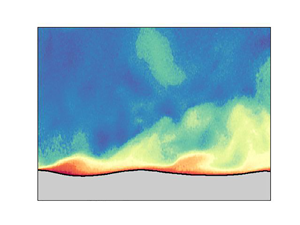
 $^{-1}$ using an optical system developed specifically to measure the turbulent airflow above wind waves. A summary of the experimental parameters is given in table 1. The experimental set-up, combining particle image velocimetry (PIV) with laser induced fluorescence (LIF) techniques, allowed us to obtain simultaneously two-dimensional velocity fields in the air above the wind-generated waves, together with spatial and temporal wave properties. The apparatus and data processing techniques are described in detail in Buckley & Veron (Reference Buckley and Veron2017) and sketched in figure 2. We have restricted our study to only a single experiment of the set described by Buckley & Veron (Reference Buckley and Veron2017), since it is the only one in which wind-generated waves exhibit a clearly resolved critical layer signature where the analysis presented in § 2 would apply. The additional experiments, not discussed herein, are at higher wind speeds and younger wave ages. Although we cannot rule out the presence of the critical layer mechanism in these experiments, we suspect that they involve different physical mechanisms.
Table 1. Parameters from the laboratory experiment.


Figure 2. Laboratory set-up at fetch 22.7 m, and a single PIV/LIF image showing the horizontal velocity field and water surface.
This experimental set-up allows the waves to grow naturally from an initially flat water surface, and leads to a surface displacement spectrum  $\phi (k)$ with variance distributed over a range of
  $k$ (figure 3). In order to account for this range of
  $k$, we consider two representative values: (i) the
  $k$ with peak variance
  $k_p$; and (ii) the centroid of the
  $\phi (k)$ distribution, represented by
  $\bar {k}$, the so-called dominant wavenumber (further support for this range of
  $k$ is presented below). The
  $\phi (k)$ spectrum was obtained by applying the linear dispersion relation for deep-water waves,
  $c = (g/k)^{1/2}$, to the frequency spectrum measured using optical wave gauges Buckley & Veron (Reference Buckley and Veron2016). The peak wavenumbers obtained differ slightly from those reported in Buckley & Veron (Reference Buckley and Veron2016), and result in a slightly different wave age, i.e.
  $c_p/u_\ast = 6.3$ versus
  $6.5$ in (Buckley & Veron Reference Buckley and Veron2016). Errors in the neglect of finite water depths and surface tension effects are at most less than 3 % at the largest relevant wavenumbers of
  $k = 100$ m
 $^{-1}$. Higher
  $k$ must be considered suspect because they may not represent freely propagating waves that satisfy the dispersion relation, but rather bound Fourier components that accompany nonlinear wave forms.

Figure 3. Wavenumber spectrum of water surface displacements with the peak ( $k_p$) and centroid (
 $\bar {k}$) wavenumber values indicated by vertical lines at
  $k_p = 46.4$ m
 $^{-1}$ and
  $\bar {k} = 62.5$ m
 $^{-1}$.
Mean profiles of velocity  $U(z)$ and shear
  $U'(z)$, obtained from the laboratory measurements, are plotted in figure 4(b). Averaging was performed with a surface following and exponentially decaying (with length scale
  $k^{-1}$) coordinate as described in Buckley & Veron (Reference Buckley and Veron2016). The profiles show classic boundary layer behaviour, with the shear concentrated very close (i.e. <1 cm) to the water surface. The location of the critical height, denoted by
  $z_c$ with
  $U(z_c) - c(k)=0$, is dependent on
  $k$, and varies between
  $1.0$ and
  $2.4$ mm for
  $k$ in the observed range
  $30~{\rm m}^{-1} \leq k \leq 100$ m
 $^{-1}$. For both
  $k = \{ k_p, \bar {k} \}$,
  $z_c$ is located less than 2 mm above the water surface (
 $1.3~{\rm mm} < z_c < 1.7$ mm; see figure 4). These small scales highlight the need for adequate resolutions of the PIV measurements that are able to resolve these scales.

Figure 4. (a) Phase-averaged vertical velocity field  $\tilde {w}(\theta,z)$ with the water layer in grey. The critical heights at
  $k = \{ k_p, \bar {k} \}$ are shown as dash-dotted and dashed lines, respectively, with the inner layer height given by the dotted line in (a–c). (b) Mean profiles of
  $U(z)$ and
  $U'(z)$ measured from the laboratory experiment. (c) Mean profile plotted on a logarithmic axis with height expressed in dimensionless wall units,
  $z_+ \equiv z u_\ast /\nu _a$. Theoretical profiles in the viscous sublayer and the logarithmic layer are indicated by the red dashed curves. The buffer layer (
 $5 \lesssim z_+ \lesssim 30$) contains the critical layer heights (grey region) and the inner layer height (dotted line). Layer definitions follow those in Kundu et al. (Reference Kundu, Cohen and Hu2004). Both the amplitude and phase of
  $\hat {w}(z)$, the vertical velocity eigenfunction, are shown in (d,e), respectively. In (d,e), the results of linear stability analysis on the profile in (b,c) are shown for two different
  $k$ corresponding to the peak
  $k_p$ and the centroid
  $\bar {k}$ of the spectrum. The horizontal grey region in (b–e) indicates the range of critical layer heights for
  $k$ between
  $\bar {k}$ and
  $k_p$. The thin vertical line in (e) indicates the optimal phase configuration for growth of
  ${\rm \pi} /2$. Note that in (d,e), we have normalised
  $\hat {w}(z)$ by the value at the water surface,
  $\hat {w}_0$.
Figure 4(c) shows  $U(z)$ with the vertical (surface following) coordinate in wall units
  $z_+ \equiv z u_\ast /\nu _a$, with
  $u_\ast \equiv (\tau /\rho _a)^{1/2}$,
  $\tau$ the shear stress, and
  $\nu _a$ the kinematic viscosity of air. We have labelled the various regions following Kundu, Cohen & Hu (Reference Kundu, Cohen and Hu2004), with the viscous sublayer at
  $z_+ \lesssim 5$, the log layer at
  $z_+ \gtrsim 30$, and the buffer layer located between them. It can be seen that the critical layer lies within the buffer layer, close to the edge of the viscous sublayer, i.e.
  $6.4 \leq z_c u_\ast / \nu _a \leq 8.0$. It is important to note that
  $U(z)$ within the buffer layer has a non-zero curvature (
 $U''(z) \neq 0$), so we may expect vorticity perturbations and behaviour in line with the linear theory presented in § 2 associated with the critical layer. This would not be the case if the critical layer was located within the viscous sublayer, where
  $U''(z) = 0$ (see also the discussion in § 3.4).
3.2. Comparison to linear theory
Given these highly resolved mean profiles, we use them as input to the linear stability analysis described in § 2. The resulting eigenfunctions of vertical velocity at  $k_p$ and
  $\bar {k}$ are shown in figures 4(b,c), along with the observed eigenfunction from the laboratory experiment. The observed
  $\hat {w}(z)$ was obtained by projecting the phase-averaged vertical velocity field
  $\tilde {w}(\theta,z)$, with
  $\theta$ the wave phase (figure 4a), onto the first-mode Fourier component via
  $\hat {w}(z) = \int _0^{2{\rm \pi} } \tilde {w}(\theta,z) \,{\rm e}^{-{\rm i}\theta } \mathrm {d} \theta / {\rm \pi}$ (see Buckley & Veron (Reference Buckley and Veron2016) for a description of the phase averaging). A close agreement between the linear stability predictions and the experiment is seen in both the general vertical variation of the amplitude, and in the phase (figures 4d,e, respectively). In particular, there is a strong variation in amplitude and phase at the location of the critical layer. Although the rapid variation with height that occurs at the critical layer appears smoother (i.e. with larger vertical length scale) in the observations, this could be due to averaging over a range of critical layer heights that arises from the range of
  $k$ found. The presence of a critical layer has important consequences for the energy transfer from wind to waves, as we discuss shortly. This classic critical layer structure has also been observed in the simulations of Sullivan, McWilliams & Moeng (Reference Sullivan, McWilliams and Moeng2000) and Kihara et al. (Reference Kihara, Hanazaki, Mizuya and Ueda2007) at similar values of wave age and slope.
The dominant  $k$ values present in the surface spectrum are also revealed in the measured eigenfunction. Since linear stability theory predicts that perturbation quantities decay exponentially with
  $z$, i.e.
  $|\hat {w}(z)| \sim {\rm e}^{-k|z|}$, far from the critical layer, it is possible to estimate
  $k$ directly from the behaviour of
  $|\hat {w}(z)|$. This is done by plotting values of
  $-\mathrm {d} (\ln |\hat {w}(z)|) /\mathrm {d} z$ for
  $z > 1.0$ cm in figure 5, as a function of
  $z$. The results generally lie between the values of
  $k_p$ and
  $\bar {k}$, supporting our focus on this range of
  $k$.
$k$.

Figure 5. Estimates of  $k$ obtained from differentiating
  $\hat {w}(z)$ in the region
  $z > 1.3$ cm.
3.3. Quantification of growth rates
Using (2.17) and the definition of  $\hat {Q} \equiv -{\rm i}kU'\hat {w}$, we can express the energy growth rate of the linear critical layer mechanism directly in terms of
  $\hat {w}$ through
 \begin{equation} \frac{\sigma_E}{r} = \mathrm{Im} \left\{ 2k\int_0^\infty {\rm e}^{{-}kz}\,\frac{U'(z)\,\hat{w}(z)}{\hat{w}_0} \,\mathrm{d} z \right\} . \end{equation}
The observed phase shift in  $\hat {w}(z)$ across the critical layer in figure 4(e) will lead to a wave-coherent pressure forcing, giving rise to an energy transfer from wind to wave. The energy growth rate
  $\sigma _E = 2\sigma$, obtained from an integration of (3.1) using the measured
  $\hat {w}(z)$ and
  $k = \{ k_p,\bar {k} \}$, is shown in figure 6(a). We refer to this growth rate estimate as the ‘linear integration’ method. In addition to this method, we also plot the growth rate curve obtained from the stability analysis of the measured
  $U(z)$, as well as three other independent predictions that we now describe.

Figure 6. (a) Comparison between the energy growth rates  $\sigma _E$ obtained from linear theory (black curve) to different methods based on the laboratory data (coloured symbols and line). The red squares labelled ‘Direct integration’ are the
  $\sigma _E/r$ values calculated directly from the laboratory observations using (2.17). The magenta line shows the growth rate obtained using the pressure reconstruction, and is independent of
  $k$. (b) Each dimensionless growth rate
  $\beta$ for the methods in (a) at
  $k_p$ is plotted onto the observations compiled by Komen et al. (Reference Komen, Cavaleri, Donelan, Hasselmann, Hasselmann and Janssen1994).
The first comes from using a recent pressure reconstruction method, described in Funke et al. (Reference Funke, Buckley, Schultze, Veron, Timmermans and Carpenter2021). For each PIV/LIF measurement, an approximate pressure field is reconstructed, and used together with an estimation of the water surface velocities to produce an energy flux. This flux is due to pressure work by the airflow on the water surface, and quantifies the rate of mechanical energy increase in the water by
 \begin{equation} \frac{\mathrm{d} }{\mathrm{d} t} E ={-}\left\langle p_0 \left( w_0 - u_0\,\frac{\partial \eta}{\partial x} \right) \right\rangle, \end{equation}
which is similar in form to the linearised version in (2.7). The water surface velocities are estimated by applying linear wave theory to the water surface elevation measurements. The energy growth rate is then found by dividing the mean energy flux (averaged over all measurements in the experiment) by the mean wave energy per unit area,  $\rho _w g a^2/2$. Note that we neglect the viscous component of the total wave energy growth since Buckley et al. (Reference Buckley, Veron and Yousefi2020) found this to have a contribution of only 3 %. The growth rate estimate thus obtained is the most direct available, and is independent of
  $k$. It is found to have mean
  $\sigma _E/r = 25.8$ rad s
 $^{-1}$ with 95 % confidence interval
  $[23.0,28.5]$ rad s
 $^{-1}$, and is plotted as a horizontal magenta line in figure 6.
The next method is approximate, and is based on the bulk momentum budget. It is described in Melville & Fedorov (Reference Melville and Fedorov2015) and Buckley et al. (Reference Buckley, Veron and Yousefi2020), with only the relevant results presented here. The energy growth rate from wind to water wave can be expressed as
 \begin{equation} \frac{\sigma_E}{r} = 2 \omega\,\frac{\tau_f}{\rho_a u_\ast^2} \left( \frac{u_\ast}{c} \right)^2 \frac{1}{(ak)^2} , \end{equation}
where we have denoted the angular wave frequency by  $\omega$, the mean form drag by
  $\tau _f$, the friction velocity by
  $u_\ast$, and the wave amplitude by
  $a$. This
  $\sigma _E$ estimate relies on approximating the wind-to-wave energy flux
  $\mathrm {d} E /\mathrm {d} t \approx c \tau _f$, by using the approximation to the surface vertical velocity from the kinematic surface condition of
  $w_0 \approx -c\,\partial \eta / \partial x$. Such an approximation neglects correlations between instantaneous fluctuations in
  $w_0$ and surface pressure that are not described by the advection of surface slopes by a single wave phase speed. The wave amplitude is quantified using the standard deviation of the interface displacement, i.e.
  $a = \sqrt {2} \, \mathrm {std}(\eta )$. Values for all of the quantities in (3.3) have previously been reported in Buckley & Veron (Reference Buckley and Veron2016), with the exception the form drag contribution. However, the latter has been determined by the pressure reconstruction method (Funke et al. Reference Funke, Buckley, Schultze, Veron, Timmermans and Carpenter2021), and found to be
  $\tau _f/(\rho _a u_\ast ^2) = 0.15$, with the remainder composed of the viscous stress. We note that this method, despite its apparent dependence on
  $k$ in (3.3), truly is a bulk measure, since it uses the bulk values of
  $\tau _f$,
  $u_\ast$ and
  $a$. The wave age
  $u_\ast /c$ and slope
  $ak$ should therefore be chosen as representative of the wave field. We apply (3.3) at both
  $k_p$ and
  $\bar {k}$, for the sake of completeness, despite it being a bulk formula. Substituting these values into (3.3) results in an energy growth rate of
  $\sigma _E /r = 32.9$ rad s
 $^{-1}$ at conditions representative of
  $k_p$.
The final growth rate estimation is due to a parametrisation of wind-wave growth by Plant (Reference Plant1982). All growth rates are plotted in figure 6(a), and are largely in agreement. In particular, at  $k_p$, the linear integration method gives a growth rate (
 $\sigma _E /r = 29.6$ rad s
 $^{-1}$) that differs from the bulk momentum budget method by only 11 %, and is only 15 % greater than that found using the pressure reconstruction (
 $\sigma _E/r = 25.8$ rad s
 $^{-1}$). All values of
  $\sigma _E$ are also found to be in agreement with previous observations, as shown in figure 6(b), where we plot the more customary dimensionless growth rate
  $\beta \equiv 2 {\rm \pi}\sigma _E / \omega$. In computing
  $\beta$, we have also subtracted the (dimensionless) viscous dissipation of wave energy
  $D = 8 {\rm \pi}\nu _w k/c = 2.3 \times 10^{-3}$, with
  $\nu _w$ the kinematic viscosity of water (see e.g. Buckley et al. Reference Buckley, Veron and Yousefi2020). We use only results at the peak wavenumber
  $k_p$ in figure 6(b).
Finally, we note that  $\beta = 9.1 \times 10^{-3}$ obtained by the bulk momentum budget differs slightly from Buckley et al. (Reference Buckley, Veron and Yousefi2020) (
 $\beta = 1.35 \times 10^{-2}$) due to our use of a different form drag fraction of total stress, obtained by the pressure reconstruction method of Funke et al. (Reference Funke, Buckley, Schultze, Veron, Timmermans and Carpenter2021), as well as slightly different wave ages and peak wavenumbers.
The energy growth rate comparison in figure 6(a) shows that for the dominant band of  $k$ observed in the experiment, all four growth rate estimates agree to within less than a factor of two. Note that this is the approximate magnitude of the error found between predictions and available measurements of wave growth (Sullivan & McWilliams Reference Sullivan and McWilliams2010). This demonstrates the main result of this paper: that the critical layer mechanism, quantified by the linear integration method, provides a significant component of the wind-to-wave energy transfer in these wind-wave conditions.
3.4. Discussion of wind-wave growth mechanisms
This result, that Miles’ critical layer mechanism provides a significant component of the wind-wave energy growth, is surprising for the growth of such young (wave age of 6.3), strongly wind-forced waves. It represents a departure from the growth mechanism classification suggested by Belcher & Hunt (Reference Belcher and Hunt1998), whereby slow waves ( $c_p/u_\ast < 15$) with critical layers that lie within the so-called inner layer should play no dynamical role. The inner layer height,
  $\ell _i$, is defined by Belcher & Hunt (Reference Belcher and Hunt1998) as the height throughout which turbulent eddies are able to adjust to the changing wave-perturbed mean flow. This height is found by an order-of-magnitude equivalence between the eddy evolution time scale
  $\kappa \ell _i/u_\ast$ and the mean flow advective time scale
  $1/(k_p|U(\ell _i) - c_p|)$, giving the following implicit equation for
  $\ell _i$:
 \begin{equation} \ell_i\,|U(\ell_i)-c_p| = \frac{2\kappa u_\ast}{k_p} . \end{equation}
Here, an additional factor  $2\kappa ^2$ is included by Belcher & Hunt (Reference Belcher and Hunt1998), where
  $\kappa = 0.4$ is the von Kármán constant, and we use conditions at
  $k_p$. This results in an inner layer height
  $\ell _i = 4.4$ mm, plotted in figure 4. We note that the turbulent boundary layer exhibits clear sheltering effects, with observable boundary layer thickening downwind of wave crests (not shown; see Buckley & Veron Reference Buckley and Veron2016). Despite this, Miles’ critical layer mechanism is able to capture the energy growth rate, as well as a close representation of the average wave-coherent flow structure.
A possible explanation for this result is the close proximity of the viscous sublayer at  $z_+ = 5$ to the inner layer height at
  $z_+ = 21$. Indeed, while turbulence normally permeates the entire inner layer, here, the proximity with the viscous and buffer layers (see figure 4c) suggests that viscous effects could be felt within the inner region. This would imply that the classification system of Belcher & Hunt (Reference Belcher and Hunt1998) based on wave age (
 $c_p/u_\ast$) would also have a dependence on an air-side wave Reynolds number
  $Re \equiv u_\ast /(k_p \nu _a)$, where
  $\nu _a$ is the kinematic viscosity of air. This can be seen by specifying the requirement that
  $\ell _i$ lie outside the buffer layer
 \begin{equation} \ell_i = \frac{2\kappa u_\ast}{|U(\ell_i) - c_p|\,k_p} > 30\,\frac{\nu_a}{u_\ast} , \end{equation}
which can be rewritten as
 \begin{equation} Re > \frac{15}{\kappa}\left| \frac{U(\ell_i)}{u_\ast} - \frac{c_p}{u_\ast} \right| . \end{equation}
Specifying the approximate mean flow at the edge of the buffer layer as  $U(\ell _i) \geq 15 u_\ast$, and restricting conditions to the slow wave regime of Belcher & Hunt (Reference Belcher and Hunt1998) with
  $c_p/u_\ast < 15$, gives the very approximate criteria
  $Re > O(10^2\unicode{x2013}10^3)$ for an inner layer height outside the buffer layer. In the present experiment,
  $Re = 100$ (accurate to two significant figures), with the inner layer within the buffer layer.
Additionally, we can quantify the contribution of the neglected terms of the wave mean flow contribution to the forcing of the pressure field through  $Q$. Within Miles’ linear theory,
  $Q$ is represented entirely by the
  $O(a)$ term
  $-U'\,\partial w/\partial x$. The additional terms of
  $Q$, consisting of
  $O(a^2)$ contributions (e.g.
  $(\partial u/\partial x)(\partial w/\partial z)$), can be approximated by taking
  $x \approx k_p^{-1} \theta$, with
  $\theta$ the phase variable in the phase-averaged
  $\tilde {Q}(\theta,z)$. However, we find that these additional terms in the wave mean
  $\tilde {Q}$ account for only 13 % of the root-mean-square variation of the
  $Q$ field. Therefore, the
  $-U'\,\partial w/\partial x$ term is dominating the
  $Q$ variation and represents the leading contribution to wave growth, as assumed in Miles’ critical layer theory.
4. Summary and conclusions
In this paper, we have presented the first quantification of Miles’ linear growth mechanism in the airflow over young (wave age 6.3) wind-generated laboratory waves. This conclusion is supported by both a comparison of the wave-coherent flow structure, showing a clear critical layer phase shift and amplitude structure that is largely in agreement with theory, and a quantification of the critical layer contribution to the wave energy growth rate that compares well to other direct and indirect bulk estimates and previous observations. The critical layer growth rate estimate is accomplished through the formulation of a new diagnostic based on linear stability theory (i.e. the technique employed by Miles Reference Miles1957) that can be applied to any wave-coherent measurements of the airflow. However, it is important to note that an extremely high resolution of the airflow above the water surface (less than 2 mm in the present case) is required to resolve the critical layer structure in such young wind waves. The identification of such a mechanism is in contrast with the previously suggested wave age classification of Belcher & Hunt (Reference Belcher and Hunt1998), whereby the growth of waves with ages smaller than 15 should be dominated by the sheltering mechanism. We suggest that at low Reynolds number, the wave age classification should also consider viscous effects. The specific dynamical role of the frequently observed sheltering events, and of the strongly wave-modulated airflow turbulence, for the wave growth of these and other higher wind speed and wave slope wind-wave conditions, remains to be investigated, and will form a basis for further work.
Acknowledgements
We acknowledge funding provided by the Helmholtz Association through the PACES II and PoF IV programmes, as well as the Deutsche Forschungsgemeinschaft (DFG). This paper is a contribution to the projects M6 and T4 of the Collaborative Research Centre TRR181, ‘Energy Transfers in Atmosphere and Ocean’ funded by the Deutsche Forschungsgemeinschaft (DFG, German Research Foundation) – grant 274762653. M.P.B. and F.V. acknowledge support from the National Science Foundation, USA (grants OCE-1458977, OCE-1233808, OCE-0748767 and AGS-PRF-1524733).
Declaration of interests
The authors report no conflict of interest.


 Open access