


1. Introduction
Evaporation in porous media is a ubiquitous phenomenon in nature and industrial applications, for example, drying of building materials after rainy days (Defraeye et al. Reference Defraeye, Houvenaghel, Carmeliet and Derome2012) and drainage in proton exchange membrane fuel cells (Wu et al. Reference Wu, Zhao, Tsotsas and Kharaghani2017). Therefore, its study is of great interest to the advancement in many fields of science and technology. Like usual evaporation phenomena, evaporation in porous media is triggered when the surrounding vapour is unsaturated, which can be achieved via (i) increasing the environmental temperature in single-component liquid–vapour systems (Qin et al. Reference Qin, Del Carro, Mazloomi Moqaddam, Kang, Brunschwiler, Derome and Carmeliet2019), (ii) decreasing the environmental pressure in isothermal single-component liquid–vapour systems (Qin et al. Reference Qin, Zhao, Kang, Derome and Carmeliet2021; Zhao et al. Reference Zhao, Qin, Kang, Derome and Carmeliet2022), (iii) decreasing the environmental vapour concentration in isothermal–isobaric multicomponent liquid–gas systems (Coussot Reference Coussot2000; Yiotis et al. Reference Yiotis, Tsimpanogiannis, Stubos and Yortsos2007) or (iv) combining different pressure, temperature and concentration gradients (Fei et al. Reference Fei, Qin, Wang, Luo, Derome and Carmeliet2022a). Evaporation in porous media is a typical multiscale problem, involving micropore to the environment lengths, convection to diffusion time scales, whose complexity is further increased with the multiple physical processes at play, such as phase change, interfacial flows and coupled heat and mass transfer (Qin et al. Reference Qin, Del Carro, Mazloomi Moqaddam, Kang, Brunschwiler, Derome and Carmeliet2019; Fei et al. Reference Fei, Qin, Zhao, Derome and Carmeliet2022b). For such a problem, the extraction of detailed information at the pore scale is challenging even with the most advanced imaging techniques. Pore-scale investigation is essential since it not only helps to elucidate the underlying mechanisms of behaviour at the macroscale, but also provides guidelines for constructing macroscopic models using various upscaling techniques, such as the homogenization technique (Whitaker Reference Whitaker1977), the volume averaging method (Ahmad et al. Reference Ahmad, Talbi, Prat, Tsotsas and Kharaghani2020) and thermodynamically constrained averaging theory (Jackson, Miller & Gray Reference Jackson, Miller and Gray2009). Besides, statistical information from pore-scale data can be used to validate the upscaled models (Lasseux & Valdés-Parada Reference Lasseux and Valdés-Parada2022). Therefore, there is an increasing need for reliable numerical models able to allow pore-scale investigations of flows in porous media coupled with liquid–vapour phase change (Ackermann, Bringedal & Helmig Reference Ackermann, Bringedal and Helmig2021; Vorhauer-Huget & Shokri Reference Vorhauer-Huget and Shokri2022).
Various numerical models have been developed to investigate evaporation in porous media, including continuum models (Defraeye Reference Defraeye2014; Le, Tsotsas & Kharaghani Reference Le, Tsotsas and Kharaghani2018), pore-network models (PNMs) (Surasani, Metzger & Tsotsas Reference Surasani, Metzger and Tsotsas2008; Wu et al. Reference Wu, Zhao, Tsotsas and Kharaghani2017; Vorhauer-Huget & Shokri Reference Vorhauer-Huget and Shokri2022) and lattice Boltzmann models (LBMs) (Qin et al. Reference Qin, Del Carro, Mazloomi Moqaddam, Kang, Brunschwiler, Derome and Carmeliet2019; Zachariah, Panda & Surasani Reference Zachariah, Panda and Surasani2019). In addition, some efforts have been made to construct multiscale models by coupling different models, such as an LBM–PNM (Zhao et al. Reference Zhao, Qin, Kang, Derome and Carmeliet2022) and a PNM–finite volume model (Weishaupt & Helmig Reference Weishaupt and Helmig2021). Increasingly used, the LBM is particularly well suited for pore-scale modelling of evaporation in porous media. Different from the continuum models, the LBM is a solver of a specific discrete Boltzmann equation, designed to recover the Navier–Stokes equations in the low-Mach-number limit (Qiand, d'Humières & Lallemand Reference Qian, d'Humières and Lallemand1992; Chen & Doolen Reference Chen and Doolen1998; Shan Reference Shan2006; Guo & Shu Reference Guo and Shu2013; Succi Reference Succi2018). The mesoscale nature of the LBM allows the natural incorporation of micro- and mesoscale physics, leading to straightforward treatment of multiphase interface dynamics, such as phase separation and breakup and/or merging of phase interfaces (Shan & Chen Reference Shan and Chen1993, Reference Shan and Chen1994; Succi Reference Succi2015; Li et al. Reference Li, Luo, Kang, He, Chen and Liu2016; Gan et al. Reference Gan, Xu, Lai, Li, Sun and Succi2022; Huang, Li & Adams Reference Huang, Li and Adams2022). Compared with PNMs, the LBM is a more accurate pore-scale method since the bounce-back type of boundary schemes in the LBM is very suitable for realistic and complex pore structures (Liu et al. Reference Liu, Kang, Leonardi, Schmieschek, Narváez, Jones, Williams, Valocchi and Harting2016; Chen et al. Reference Chen, He, Zhao, Kang, Li, Carmeliet, Shikazono and Tao2022), discarding the need for large simplification of real geometries. Finally, the ‘collision-streaming’ algorithm in the standard LBM involves information exchange only among neighbouring lattice nodes, making it highly efficient in large-scale parallel computations (Peng, Ayala & Wang Reference Peng, Ayala and Wang2019; Fei et al. Reference Fei, Yang, Chen, Mo and Luo2020; Peng, Ayala & Wang Reference Peng, Ayala and Wang2020; Wang, Fei & Luo Reference Wang, Fei and Luo2022).
In 2013, El Abrach, Dhahri & Mhimid (Reference El Abrach, Dhahri and Mhimid2013) proposed the simulation of heat and mass transfer during drying of deformable porous media using the LBM. In their model, the porous media are modelled at the representative element volume scale, which, however, did not resolve pore-scale information. Recently, the LBM has been extended to simulate single-component evaporation in porous media at pore scales. Qin et al. (Reference Qin, Del Carro, Mazloomi Moqaddam, Kang, Brunschwiler, Derome and Carmeliet2019) constructed a hybrid non-isothermal LBM to study the evaporation in synthetic pore structures driven by temperature gradient and achieved satisfactory agreement with experiment results. In their model, the flow fields of liquid and vapour are solved by a single-component pseudopotential LBM and the temperature field by a finite-difference scheme. Further coupling to a nanoparticle transport model allows the investigation of nanoparticle depositions during drying in porous media (Qin et al. Reference Qin, Su, Zhao, Moqaddam, Del Carro, Brunschwiler, Kang, Song, Derome and Carmeliet2020). We note that, in many cases, although a temperature variation may occur due to latent heat, the evaporation is mainly driven by the vapour concentration gradient (Coussot Reference Coussot2000; Yiotis et al. Reference Yiotis, Tsimpanogiannis, Stubos and Yortsos2007). For such evaporation, the diffusion among gas components, e.g. dry air and water vapour, needs to be taken into account. Therefore, a multicomponent approach considering component diffusion is more suitable and allows one to model also the developing vapour boundary layers. Based on a multicomponent pseudopotential LBM, Zachariah et al. (Reference Zachariah, Panda and Surasani2019) proposed a two-component isothermal model to investigate invasion patterns and cluster formation during convective drying of porous media. However, the convective inflow Reynolds number (Re) range is limited to values smaller than 0.05, possibly because the adopted LBM collision, forcing and boundary schemes are limited to low-Re problems. In addition, the ability of multicomponent LBMs to simulate the effect of non-condensible gas (NCG) and component diffusion in gas mixtures is still not yet satisfactorily explored. In the literature, the concentration of NCG is mainly limited to small values (Zheng et al. Reference Zheng, Eimann, Philipp, Fieback and Gross2019; Fei et al. Reference Fei, Qin, Zhao, Derome and Carmeliet2022b), i.e. 1 %–2 % and 10 %–15 % under non-isothermal and isothermal evaporation cases, respectively, which are much smaller than the value in the natural environment ( ${>}97\,\%$).
In the work described above, the LBMs for multicomponent evaporation are not sufficiently developed, making it challenging for a systematic study of the drying of porous media in wide governing parameter ranges. As the first step towards this problem, we simplify the system to be of two components (Shokri, Lehmann & Or Reference Shokri, Lehmann and Or2009), one a volatile component (water and its vapour) and the other a NCG (dry air). We further consider the isothermal evaporation in porous media, where the evaporation is induced by a vapour concentration gradient from the unsaturated gas mixture to the liquid–gas interface. Recently, we have proposed to model such evaporation phenomena based on the two-component two-phase pseudopotential LBM (Shan & Chen Reference Shan and Chen1993, Reference Shan and Chen1994). However, a detailed model analysis is still missing and the preliminary simulations are limited to a small dry air concentration ( ${\leqslant }15\,\%$) and narrow contact angle range (
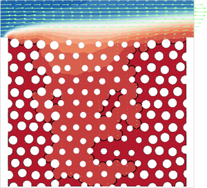
 ${20^\circ } \leqslant \theta \leqslant {60^\circ }$) (Fei et al. Reference Fei, Qin, Zhao, Derome and Carmeliet2022b). In this work, we particularly aim to describe the model in detail regarding the diffusion mechanism, the achievement of large dry air concentration in the gas phase and the implementation of a wider contact angle range in the two-component system. In addition, applications of the model to convective evaporation of a dual-porosity medium are presented, and parametric studies are carried out. We aim to demonstrate that the proposed numerical model can be used to simulate the pore-scale interface dynamics of two-component evaporation in heterogeneous porous media at moderate Reynolds number with wide ranges of contact angle and water vapour concentration.
The remainder of the paper is organized as follows. In § 2, we give the details of model development and theoretical analysis. The achievement of a large dry air mass fraction, the implementation of wettability on the curved boundary in the two-component two-phase system and the validation of the model with microfluidic experiments are given in § 3. The application of the model to convective evaporation in a specifically designed dual-porosity medium is presented and a systematic study is carried out in § 4. Finally, in § 5, we evaluate the proposed model and conclude the paper.
2. Model development
In this section, a two-component LBM is constructed to simulate isothermal two-component flows. In the lattice Boltzmann community, various collision schemes, such as those of single relaxation time (Qian et al. Reference Qian, d'Humières and Lallemand1992), multiple relaxation time (Lallemand & Luo Reference Lallemand and Luo2000), cascaded or central moment (Geier, Greiner & Korvink Reference Geier, Greiner and Korvink2006) and entropic multiple relaxation time (Karlin, Bösch & Chikatamarla Reference Karlin, Bösch and Chikatamarla2014), can be employed to suit the problems under investigation. These schemes have been discussed in detail and integrated into a unified framework (Luo, Fei & Wang Reference Luo, Fei and Wang2021). In this work, the cascaded scheme is used as it possesses excellent numerical stability (Geier et al. Reference Geier, Greiner and Korvink2006; Fei et al. Reference Fei, Yang, Chen, Mo and Luo2020), while it allows achieving non-slip boundary condition (Fei & Luo Reference Fei and Luo2017; Fei, Luo & Li Reference Fei, Luo and Li2018a) and tuning the Schmidt number (as shown below). To mimic the isothermal liquid–vapour phase change, we propose to appropriately incorporate two-component two-phase pseudopotential interactions (Shan & Chen Reference Shan and Chen1993, Reference Shan and Chen1994) into the present model. Finally, to deal with different wettability, the geometry-function-based contact angle scheme, originally developed for single-component systems (Ding & Spelt Reference Ding and Spelt2007; Li, Yu & Luo Reference Li, Yu and Luo2019), is extended to two-component systems. The present work is limited to two dimensions.
2.1. Two-component cascaded LBM
Following the standard LBM algorithm, the cascaded LBM (CLBM) first executes the collision in the central moment space, then the post-collision distributions are reconstructed from their central moments and finally the streaming step is carried out in discrete velocity space. Here, a raw moment is the moment representation of the density distribution functions (DDFs) based on the discrete velocity set, and a central moment corresponds to a raw moment displaced by the macroscopic fluid velocity, as defined in the following (equation (2.5a,b)). The above-mentioned steps can be integrated into a uniform framework (Fei & Luo Reference Fei and Luo2017; Fei et al. Reference Fei, Luo and Li2018a; Luo et al. Reference Luo, Fei and Wang2021), written as the following two-component cascaded lattice Boltzmann equation:
 \begin{align} f_i^k(\boldsymbol{x} +
{\boldsymbol{e}_i}\Delta t,t + \Delta t) &= f_i^k\left(
{\boldsymbol{x},t} \right) - ({{\boldsymbol{\mathsf{M}}}^{ -
1}}{{\boldsymbol{\mathsf{N}}^{ - 1}}}{
\boldsymbol{\mathsf{S}}}{\boldsymbol{\mathsf{N}}}{\boldsymbol{\mathsf{M}}})\left.\left({f_i^k - f_i^{k,eq}} \right)\right|_{\left({\boldsymbol{x},t} \right)}\nonumber\\
&\quad + \frac{{\Delta t}}{2}\left[ {R_i^k\left| _{\left({\boldsymbol{x},t} \right)} \right.
+ R_i^k\left| _{\left({\boldsymbol{x} + {\boldsymbol{e}_i}\Delta t,t + \Delta t}\right)}\right.}\right],
\end{align}
\begin{align} f_i^k(\boldsymbol{x} +
{\boldsymbol{e}_i}\Delta t,t + \Delta t) &= f_i^k\left(
{\boldsymbol{x},t} \right) - ({{\boldsymbol{\mathsf{M}}}^{ -
1}}{{\boldsymbol{\mathsf{N}}^{ - 1}}}{
\boldsymbol{\mathsf{S}}}{\boldsymbol{\mathsf{N}}}{\boldsymbol{\mathsf{M}}})\left.\left({f_i^k - f_i^{k,eq}} \right)\right|_{\left({\boldsymbol{x},t} \right)}\nonumber\\
&\quad + \frac{{\Delta t}}{2}\left[ {R_i^k\left| _{\left({\boldsymbol{x},t} \right)} \right.
+ R_i^k\left| _{\left({\boldsymbol{x} + {\boldsymbol{e}_i}\Delta t,t + \Delta t}\right)}\right.}\right],
\end{align}
where  $f_i^k(\boldsymbol {x},t)$ is the DDF of component
  $k$ (
$k$ ( $=A,B$) at the space–time position
  $(\boldsymbol {x},t)$, moving along the ith lattice direction by discrete velocities
  ${\boldsymbol {e}_i}$. The left-hand side of (2.1) represents molecular free streaming, while the right-hand side stands for time relaxation towards the local equilibrium state due to molecular collisions and
  $R_i^k(\boldsymbol x,t)$ are the forcing terms in discrete velocity space. To eliminate the implicitness, (2.1) can be rewritten by introducing
  $\bar {f}_i^k = f_i^k - 0.5\Delta tR_i^k$:
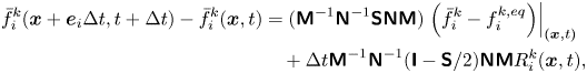 \begin{align} \bar{f}_i^k(\boldsymbol{x} + {\boldsymbol{e}_i}\Delta t,t + \Delta t) - \bar{f}_i^k(\boldsymbol{x},t) &= ({{\boldsymbol{\mathsf{M}}}^{ - 1}}{\boldsymbol{\mathsf{N}}^{ - 1}}{ \boldsymbol{\mathsf{SN}}}{\boldsymbol{\mathsf{M}}})\left.\left( {\bar{f}_i^k - f_i^{k,eq}} \right)\right|_{(\boldsymbol{x},t)} \nonumber\\ &\quad +\Delta t{{\boldsymbol{\mathsf{M}}}^{ - 1}}{\boldsymbol{\mathsf{N}}^{ - 1}}({\boldsymbol{\mathsf{I}}} - {\boldsymbol{\mathsf{S}}}/2){\boldsymbol{\mathsf{NM}}}R_i^k(\boldsymbol{x},t), \end{align}
where  ${\boldsymbol{\mathsf{I}}}$ is the unit matrix and
  $\boldsymbol{\mathsf{S}}$ is the relaxation matrix, whose elements are the relaxation rates for each central moment. The transformation matrix
  $\boldsymbol{\mathsf{M}}$ is used to transfer
  $\bar {f}_i^k$ to their raw moments
  $T_i^k$, as does the shift matrix
  $\boldsymbol{\mathsf{N}}$ for the shift between
  $T_i^k$ and the central moments
  $\tilde {T}_i^k$, namely
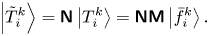 \begin{equation} \left| {\tilde{T}_i^k} \right\rangle = {\boldsymbol{\mathsf{N}}}\left| {T_i^k} \right\rangle = {\boldsymbol{\mathsf{NM}}}\left| {\bar{f}_i^k} \right\rangle . \end{equation}
 In this work, the two-dimensional nine-velocity lattice (D2Q9) (Qian et al. Reference Qian, d'Humières and Lallemand1992) is used. The lattice speed  $c = \Delta x/\Delta t = 1$ and the lattice sound speed
  ${c_s} = c/\sqrt 3$ are adopted, with lattice spacing
  $\Delta x=1$ and time step
  $\Delta t=1$. The discrete velocities
  ${\boldsymbol {e}_i} = [ {| {{e_{ix}}} \rangle,| {{e_{iy}}} \rangle } ]$ (
 $i = 0,1, \ldots,8$) are defined as
 \begin{equation} \left.\begin{gathered} |{e_{ix}}\rangle = [0, 1, -1, 0, 0, 1, -1, 1, -1]^\top, \\ |{e_{iy}}\rangle = [0, 0, 0, 1, -1, 1, -1, -1, 1]^\top. \end{gathered}\right\} \end{equation}
Let us use the symbols  $|{\cdot }\rangle $ and
  $\top$ to denote a nine-column vector and the transpose operator, respectively. To construct the CLBM, the raw and central moments of
  $\bar {f}_i^k$ are introduced:
 \begin{equation} k_{mn}^k = \left\langle {\bar{f}_i^k|e_{ix}^me_{iy}^n} \right\rangle {{,\quad}}\tilde{k}_{mn}^k = \left\langle {\bar{f}_i^k|{{\left( {{e_{ix}} - {u_x}} \right)}^m}{{\left( {{e_{iy}} - {u_y}} \right)}^n}} \right\rangle , \end{equation}
where  $\boldsymbol {u} = [ {{u_x},{{ }}{u_y}} ]$ is the macroscopic velocity of the two-component mixture and m and n are positive integers. The equilibrium raw and central moments,
  $k_{mn}^{k,eq}$ and
  $\tilde {k}_{mn}^{k,eq}$, are defined consistently by replacing
  $\bar {f}_i^k$ with their equilibrium counterparts
  $f_i^{k,eq}$. Then, one needs to choose an appropriate moment set. As suggested in Geier et al. (Reference Geier, Greiner and Korvink2006), Fei & Luo (Reference Fei and Luo2017), Premnath & Banerjee (Reference Premnath and Banerjee2009), Fei et al. (Reference Fei, Luo, Lin and Li2018b) and De Rosis (Reference De Rosis2017), the following raw moment set is used in the present work:
 \begin{equation} \left| {T_i^k} \right\rangle = {\left[ {k_{00}^k,k_{10}^k,k_{01}^k,k_{20}^k + k_{02}^k,k_{20}^k - k_{02}^k,k_{11}^k,k_{21}^k,k_{12}^k,k_{22}^k} \right]^{\top}}, \end{equation}
and accordingly the central moment set  $\tilde {T}_i^k$ is determined. In (2.6), the first three moments represent the component density and momentum, and the middle and last three stand for the viscous stress and high-order non-hydrodynamic moments, respectively. For such a choice, one can write
  $\boldsymbol{\mathsf{M}}$ and
  $\boldsymbol{\mathsf{N}}$ explicitly according to the relation in (2.3):
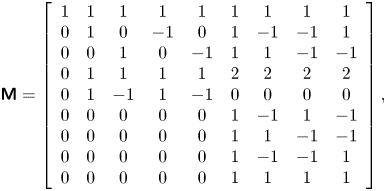 \begin{gather} {\boldsymbol{\mathsf{M}}} = \left[ {\begin{array}{ccccccccc} 1 & 1 & 1 & 1 & 1 & 1 & 1 & 1 & 1\\ 0 & 1 & 0 & { - 1} & 0 & 1 & { - 1} & { - 1} & 1\\ 0 & 0 & 1 & 0 & { - 1} & 1 & 1 & { - 1} & { - 1}\\ 0 & 1 & 1 & 1 & 1 & 2 & 2 & 2 & 2\\ 0 & 1 & { - 1} & 1 & { - 1} & 0 & 0 & 0 & 0\\ 0 & 0 & 0 & 0 & 0 & 1 & { - 1} & 1 & { - 1}\\ 0 & 0 & 0 & 0 & 0 & 1 & 1 & { - 1} & { - 1}\\ 0 & 0 & 0 & 0 & 0 & 1 & { - 1} & { - 1} & 1\\ 0 & 0 & 0 & 0 & 0 & 1 & 1 & 1 & 1 \end{array}}\right],\end{gather}
 \begin{gather} {\boldsymbol{\mathsf{N}}}=\left[\begin{array}{@{}ccccccccc@{}} 1 & 0 & 0 & 0 & 0 &0 & 0 & 0 & 0\\ { - {u_x}} & 1 & 0 & 0 & 0&0 & 0 & 0 & 0\\ { - {u_y}} & 0 & 1 & 0 & 0&0 & 0 & 0 & 0\\ {u_x^2 + u_y^2} & { - 2{u_x}} & { - 2{u_y}} & 1 & 0 &0 & 0 & 0 & 0\\ {u_x^2 - u_y^2} & { - 2{u_x}} & {2{u_y}} & 0 & 1 &0 & 0 & 0 & 0\\ {{u_x}{u_y}} & { - {u_y}} & { - {u_x}} & 0 & 0 &1 & 0 & 0 & 0\\ { - u_x^2{u_y}} & {2{u_x}{u_y}} & {u_x^2} & { - {u_y}/2} & { - {u_y}/2} &{ - 2{u_x}} & 1 & 0 & 0\\ { - u_y^2{u_x}} & {{u_y}^2} & {2{u_x}{u_y}} & { - {u_x}/2} & {{u_x}/2} &{ - 2{u_y}} & 0 & 1 & 0\\ {u_x^2u_y^2} & { - 2{u_x}u_y^2} & { - 2{u_y}u_x^2} & {u_x^2/2 + u_y^2/2} & {u_y^2/2 - u_x^2/2} &{4{u_x}{u_y}} & { - 2{u_y}} & { - 2{u_x}} & 1 \end{array}\right]. \end{gather}
Due to the physical definitions of  $\boldsymbol{\mathsf{M}}$ and
  $\boldsymbol{\mathsf{N}}$, both of them are invertible. Moreover,
  $\boldsymbol{\mathsf{N}}^{-1}$ has a quite similar formulation to
  $\boldsymbol{\mathsf{N}}$, and can be obtained by reversing all the odd-order velocity terms in (2.8). For more details, the interested reader is directed to Fei & Luo (Reference Fei and Luo2017). In addition, the relaxation matrix is diagonal,
  ${\boldsymbol{\mathsf{S}}} = \textrm {diag}( {{s_0},{s_1},{s_1},{s_b},{s_v},{s_v},{s_3},{s_3},{s_4}} )$, where we consider the relaxation rates identical for each component.
In the numerical implementation, the matrix calculations for  $f_i^{k,eq}$ and
  $R_i^{k}$ are not needed because their central moments are defined by matching the continuous integration of the Maxwellian distribution (Fei & Luo Reference Fei and Luo2017; Fei et al. Reference Fei, Luo, Lin and Li2018b):
 \begin{equation} \left.\begin{gathered} \left\langle {f_i^{k,eq}|{{\left( {{e_{ix}} - {u_x}} \right)}^m}{{\left( {{e_{iy}} - {u_y}} \right)}^n}} \right\rangle = \int_{ - \infty }^{ + \infty } {\int_{ - \infty }^{ + \infty } {f_M^k{{({\xi _x} - {u_x})}^m}{{({\xi _y} - {u_y})}^n}\,{\rm d}} } {\xi _x}\,{\rm d}{\xi _y}, \\ \left\langle {R_i^k|{{\left( {{e_{ix}} - {u_x}} \right)}^m}{{\left( {{e_{iy}} - {u_y}} \right)}^n}} \right\rangle = \int_{ - \infty }^{ + \infty } {\int_{ - \infty }^{ + \infty } {R_M^k{{({\xi _x} - {u_x})}^m}{{({\xi _y} - {u_y})}^n}\,{\rm d}} } {\xi _x}\,{\rm d}{\xi _y}, \end{gathered}\right\} \end{equation}
where  $f_M^k$ is the Maxwellian equilibrium distribution in continuous velocity space
  ${\boldsymbol {\xi }} = [{\xi _x},{\xi _y}]$ for molecules of component k and
  $R_M^k$ is the forcing effect approximation in the Boltzmann equation of He, Chen & Doolen (Reference He, Chen and Doolen1998). As a result, the equilibrium central moments and the forcing terms in the central moment space (
 $| {C_i^k} \rangle = {\boldsymbol{\mathsf{NM}}}| {R_i^k} \rangle$) can be obtained (Fei & Luo Reference Fei and Luo2017):
 \begin{equation} \left.\begin{gathered} \left| {\tilde{T}_i^{k,eq}} \right\rangle = {\left[ {{\rho_k},0,0,2{\rho_k}c_s^2,0,0,0,0,{\rho_k}c_s^4} \right]^\top},\\ \left| {C_i^k} \right\rangle = {\left[ {0,F_x^k,F_y^k,0,0,0,F_y^kc_s^2,F_x^kc_s^2,0} \right]^\top}, \end{gathered}\right\} \end{equation}
where  ${\rho _k}$ and
  ${{\boldsymbol {F}}^k} = [F_x^k,F_y^k]$ are the component density and forcing field, respectively. Based on the above definitions, one can solve
  $\bar {f}_i^k$ by iterating (2.1). After each iteration step, the macroscopic variables are updated by (Shan & Chen Reference Shan and Chen1993; Chai & Zhao Reference Chai and Zhao2012)
 \begin{equation} \rho = \sum\limits_k {{\rho _k}} = \sum\limits_k {\sum\limits_i {\bar{f}_i^k} } ,\quad{{ }}\rho {\boldsymbol{u}} = \sum\limits_k {{\rho _k}{{\boldsymbol{u}}_k}} = \sum\limits_k {\left( {\sum\limits_i {\bar{f}_i^k} {{\boldsymbol{e}}_i} + 0.5\Delta t{{\boldsymbol{F}}^k}} \right)} . \end{equation}
Using the Chapman–Enskog analysis (see Appendix A), the above two-component CLBM reproduces the following macroscopic Navier–Stokes equations and the convective–diffusion equation for the mixture fluid in the low-Mach limit:
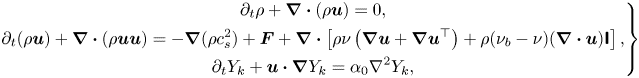 \begin{equation} \left.\begin{gathered} {\partial _t}\rho + \boldsymbol{\nabla} \boldsymbol{\cdot} (\rho {\boldsymbol{u}}) = 0,\\ {\partial _t}(\rho {\boldsymbol{u}}) + \boldsymbol{\nabla} \boldsymbol{\cdot} (\rho {\boldsymbol{uu}}) ={-} \boldsymbol{\nabla} (\rho c_s^2) + {\boldsymbol{F}} + \boldsymbol{\nabla}\boldsymbol{\cdot} \left[ {\rho \nu \left( {\boldsymbol{\nabla} {\boldsymbol{u}} + \boldsymbol{\nabla} {{\boldsymbol{u}}^{\top}}} \right) + \rho ({\nu _b} - \nu )( \boldsymbol{\nabla}\boldsymbol{\cdot} {\boldsymbol{u}}){\boldsymbol{\mathsf{I}}}} \right],\\ {\partial _t}{Y_k} + {\boldsymbol{u}} \boldsymbol{\cdot}\boldsymbol{\nabla} {Y_k} = {\alpha _0}{\nabla ^2}{Y_k} , \end{gathered}\right\} \end{equation}
where  ${\boldsymbol {F}} = \sum \nolimits _k {{{\boldsymbol {F}}^k}}$ is the force field imposed on the system,
  ${Y_k} = {\rho _k}/\rho$ is the component mass fraction and
  $\nu = c_s^2\Delta t(1/{s_v} - 1/2)$,
  ${\nu _b} = c_s^2\Delta t(1/{s_b} - 1/2)$ and
  ${\alpha _0} = (1/s_1^k - 1/2)c_s^2\Delta t$ are the mixture kinetic viscosity, bulk viscosity and binary diffusivity, respectively. Here, it may be noted that the kinetic viscosity and binary diffusivity can be tuned independently due to the use of the cascaded collision scheme, relaxing the limitation of the unity Schmidt number (
 $Sc = \nu /{\alpha _0} = 1.0$) in the classical single-relaxation-time scheme. Due to mass conservation, the first relaxation rate can be chosen arbitrarily and is fixed as
  ${s_0} = 1.0$ in the following. Unless otherwise specified, the other relaxation rates are set as
  ${s_3} = (16 - 8{s_2})/(8 - {s_2})$ and
  ${s_4}=1.0$ to achieve the non-slip boundary condition (Pan, Luo & Miller Reference Pan, Luo and Miller2006; Guo & Zheng Reference Guo and Zheng2008; Fei & Luo Reference Fei and Luo2017) while maintaining numerical stability.
2.2. Two-component two-phase pseudopotential interactions
In our case, the water component ( $k = A$) is the phase-change component, which means the intra-component interaction between liquid water and its vapour must be taken into account. The non-condensible dry air component (
 $k = B$) is miscible with water vapour but almost insoluble in liquid water. To mimic such behaviours, an appropriate inter-component interaction is needed. To this aim, we use the pseudopotential interaction model originally proposed by Shan & Chen (Reference Shan and Chen1993, Reference Shan and Chen1994), due to its simplicity in implementation and in handling different types of isothermal or non-isothermal multiphase systems (Li et al. Reference Li, Kang, Francois, He and Luo2015; Fei et al. Reference Fei, Du, Luo, Succi, Lauricella, Montessori and Wang2019; Qin et al. Reference Qin, Del Carro, Mazloomi Moqaddam, Kang, Brunschwiler, Derome and Carmeliet2019; Fei et al. Reference Fei, Yang, Chen, Mo and Luo2020; Wang et al. Reference Wang, Fei and Luo2022). The following intra- and inter-component interaction forces are used:
 \begin{equation} \left.\begin{gathered}
{{\boldsymbol{F}}_{AA}} ={-} {G_{AA}}\psi
({\boldsymbol{x}})\sum_{i {\ne} 0} {w\left( {{{\left| {{{
\boldsymbol{e}}_i}} \right|}^2}} \right)} \psi
({\boldsymbol{x}} + {{\boldsymbol{e}}_i} \Delta
t){{\boldsymbol{e}}_i},\\ {{\boldsymbol{F}}_{AB}} ={-}
{G_{AB}}{\rho _A}({\boldsymbol{x}})\sum_{i {\ne} 0} {w\left(
{{{\left| {{{\boldsymbol{e}}_i}} \right|}^2}} \right)}
{\rho _B}({\boldsymbol{x}} + {{\boldsymbol{e}}_i}\Delta
t){{\boldsymbol{e}}_i}, \end{gathered}\right\}
\end{equation}
\begin{equation} \left.\begin{gathered}
{{\boldsymbol{F}}_{AA}} ={-} {G_{AA}}\psi
({\boldsymbol{x}})\sum_{i {\ne} 0} {w\left( {{{\left| {{{
\boldsymbol{e}}_i}} \right|}^2}} \right)} \psi
({\boldsymbol{x}} + {{\boldsymbol{e}}_i} \Delta
t){{\boldsymbol{e}}_i},\\ {{\boldsymbol{F}}_{AB}} ={-}
{G_{AB}}{\rho _A}({\boldsymbol{x}})\sum_{i {\ne} 0} {w\left(
{{{\left| {{{\boldsymbol{e}}_i}} \right|}^2}} \right)}
{\rho _B}({\boldsymbol{x}} + {{\boldsymbol{e}}_i}\Delta
t){{\boldsymbol{e}}_i}, \end{gathered}\right\}
\end{equation}
where  $\psi ({\boldsymbol {x}})$ is the pseudopotential function and
  $w$ is the interaction weight with
  $w(1) = 1/3$ and
  $w(2) = 1/12$. Parameters
  ${G_{AA}}$ and
  ${G_{BB}}$ are interaction strengths. Due to the symmetry, we have
  ${{\boldsymbol {F}}_{AB}} = {{\boldsymbol {F}}_{BA}}$.
To incorporate the non-ideal gas equation of state (EOS) for the description of the water-to-vapour phase transition, the following pseudopotential function is employed (Yuan & Schaefer Reference Yuan and Schaefer2006):
 \begin{equation} \psi = \sqrt {\frac{{2({p_{EOS}} - {\rho _A}c_s^2)}}{{{G_{AA}}{c^2}}}}, \end{equation}
where  ${G_{AA}}=-1$ and
  ${p_{EOS}}$ is the pressure calculated by the EOS. Here, the Peng–Robinson non-ideal gas EOS is applied (Peng & Robinson Reference Peng and Robinson1976):
 \begin{equation} {p_{EOS}} = \frac{{{\rho _A}RT}}{{1 - b{\rho _A}}} - \frac{{a\varphi (T)\rho _A^2}}{{1 + 2b{\rho _A} - {b^2}\rho _A^2}}, \end{equation}
where  $\varphi (T) = {[1 + (0.37464 + 1.54226\varpi - 0.26992{\varpi ^2})(1 - \sqrt {T/{T_{cr}}} )]^2}$, with the acentric factor
  $\varpi =0.344$, and
  $R = 1$ is the gas constant. The critical pressure
  ${p_{cr}}$ and temperature
  ${T_{cr}}$ are determined by
  $a = 0.4572{R^2}T_{cr}^2/{p_{cr}}$ and
  $b = 0.0778R{T_{cr}}/{p_{cr}}$ (Peng & Robinson Reference Peng and Robinson1976). When such a square-root-form pseudopotential in (2.14) is used, the system suffers from the so-called thermodynamic inconsistency that the liquid–vapour coexistence densities by the mechanical stability solution deviate from those of the Maxwell construction. To solve the problem, Li, Luo & Li (Reference Li, Luo and Li2012, Reference Li, Luo and Li2013) proposed adjusting the mechanical stability condition to be consistent with the Maxwell construction. Recently, such an adjustment method has been extended to the CLBM for single-component non-isothermal multiphase systems, such as 2-D convective boiling (Saito et al. Reference Saito, De Rosis, Fei, Luo, Ebihara, Kaneko and Abe2021) and three-dimensional (3-D) pool boiling (Fei et al. Reference Fei, Yang, Chen, Mo and Luo2020). For the present two-component multiphase system, the central-moment forcing terms for the water component in (2.10) are slightly modified:
 \begin{equation} \left| {C_i^A} \right\rangle = {\left[ {0,F_x^A,F_y^A,\eta ,0,0,F_y^Ac_s^2,F_x^Ac_s^2,\eta c_s^2} \right]^{\rm T}}, \end{equation}
where  $\eta = 4\sigma {| {{{\boldsymbol {F}}_{AA}}} |^2}/[{\psi ^2}\Delta t(1/{s_b} - 0.5)]$ with an adjustment factor
  $\sigma$, whereas no adjustment is needed for the dry air component. Based on the interaction forces in (2.13), the total pressure of the system is given by
 \begin{equation} p = {p_{EOS}} + {\rho _B}c_s^2 + {G_{AB}}{\rho _A}{\rho _B}, \end{equation}
where the first and second terms are the component partial pressure according to the EOSs and the third term is the pressure contribution due to the inter-component interaction.
We stress that in (2.12) the binary diffusivity is derived based on the ideal gas EOS for each component, i.e.  ${p_k} = {\rho _k}c_s^2$. However, in this subsection, to describe the phase transition in the water component, its EOS has been updated as the non-ideal gas EOS in (2.15). Thermodynamically, water vapour can be assumed to be an ideal gas, but its equivalent sound speed in the vapour region of the Peng–Robinson EOS is different from
  ${c_s}$, leading to a deviation of the effective binary diffusivity
  $\alpha$ from the theoretical diffusivity
  ${\alpha _0}$ in (2.12). In the following, the effective binary diffusivity
  $\alpha$ is obtained based on canonical tests.
2.3. Geometric-function-based two-component contact angle scheme
To simulate evaporation in porous media, a numerical scheme is required to implement the contact angle at curved solid boundaries. In the pseudopotential LBM, the contact angle is often realized by employing another solid–fluid interaction at the boundary nodes (Martys & Chen Reference Martys and Chen1996; Li et al. Reference Li, Luo, Kang and Chen2014) or specifying a constant virtual wall density/pseudopotential (Benzi et al. Reference Benzi, Biferale, Sbragaglia, Succi and Toschi2006) when calculating the pseudopotential interactions in (2.13). They are often denoted as the solid–fluid interaction scheme and the virtual-density scheme, respectively. As discussed by Li et al. (Reference Li, Yu and Luo2019), the solid–fluid interaction scheme leads to large spurious currents, and the virtual-density scheme produces an artificial liquid film near the solid boundary. For evaporation in porous media, such artificial liquid film results in reconnection of the otherwise discontinuous liquid network, like the effect of a corner film (Chauvet et al. Reference Chauvet, Duru, Geoffroy and Prat2009), leading to higher evaporation rate. Moreover, in both the two schemes, the local geometry information (e.g. local curvature) is not explicitly incorporated, indicating inconsistency of measured contact angles in different pore structures, as also noted in Coelho et al. (Reference Coelho, Moura, Telo da Gama and Araújo2021).
Alternatively, one can accurately implement the contact angle in complex geometries using a geometric function scheme originally proposed for a phase-field method (Ding & Spelt Reference Ding and Spelt2007). Such a method was recently extended to the pseudopotential LBM by Li et al. (Reference Li, Yu and Luo2019) and further coupled with contact angle hysteresis by Qin et al. (Reference Qin, Zhao, Kang, Derome and Carmeliet2021), while still limited to single-component multiphase systems. In this work, we extend this method to two-component multiphase systems. The geometric formulation scheme also allocates a solid density value to the solid point so that the required contact angle is achieved by substituting the density into the interactions in (2.13), but the solid density is self-adaptive at each lattice node at every time step, rather than a constant value as in the virtual density scheme. As sketched in figure 1, the dashed curve is the physical boundary and the solid zigzag line  $\partial w$ connects all the solid nodes neighbouring the flow field. To achieve a prescribed contact angle
  ${\theta _p}$ at a solid point
  $S \in \partial w$, a solid density of the water component is given by (Li et al. Reference Li, Yu and Luo2019)
 \begin{equation} {\rho _{A,S}} = \left\{\begin{array}{@{}ll} \max({\rho _{A,{D_1}}},{\rho _{A,{D_2}}}), & {{}}{\theta _p} \leqslant {\rm \pi}/2,\\ \min({\rho _{A,{D_1}}},~{\rho _{A,{D_2}}}), & {{}}{\theta _p} > {\rm \pi}/2, \end{array} \right. \end{equation}
where  ${\rho _{A,{D_1}}}$ and
  ${\rho _{A,{D_2}}}$ are the densities at the two interaction points
  ${D_1}$ and
  ${D_2}$ along two characteristic lines
  ${L_1}$ and
  ${L_2}$. If
  ${D_1}$ and
  ${D_2}$ are located between liquid points, as the case in figure 1(a),
  ${\rho _{A,{D_1}}}$ and
  ${\rho _{A,{D_2}}}$ are calculated by linear interpolation. Otherwise, linear extrapolation schemes are used. The two characteristic lines are in the directions of the two unit vectors
  ${\boldsymbol {l}_1}$ and
  ${\boldsymbol {l}_2}$, defined as
 \begin{equation} \left.\begin{gathered} {\boldsymbol{l}_1} = \left[ {{n_{s,x}}\cos ({\theta _c}) - {n_{s,y}}\sin ({\theta _c}),{{}}{n_{s,x}}\sin ({\theta _c}) + {n_{s,y}}\cos ({\theta _c})} \right],\\ {\boldsymbol{l}_2} = \left[ {{n_{s,x}}\cos ({\theta _c}) + {n_{s,y}}\sin ({\theta _c}), - {n_{s,x}}\sin ({\theta _c}) + {n_{s,y}}\cos ({\theta _c})} \right], \end{gathered}\right\} \end{equation}
where  ${\theta _c} = {\rm \pi}/2 - {\theta _p}$ is the complementary angle and
  ${\boldsymbol {n}_s} = [ {{n_s}_x,{{}}{n_s}_y} ]$ is the normal vector of the curved surface at the local point S. Following Li et al. (Reference Li, Yu and Luo2019) and Qin et al. (Reference Qin, Zhao, Kang, Derome and Carmeliet2021),
  ${\boldsymbol {n}_s}$ is evaluated by the eighth-order isotropic scheme based on the D2Q25 lattice (figure 1b):
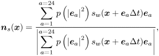 \begin{equation} {\boldsymbol{n}_s}({\boldsymbol{x}}) = \frac{\displaystyle{\sum_{a = 1}^{a = 24} {p\left( {{{\left| {{{\boldsymbol{e}}_a}} \right|}^2}} \right){s_w}({\boldsymbol{x}} + {{\boldsymbol{e}}_a}\Delta t){{\boldsymbol{e}}_a}} }}{{\displaystyle\left| {\sum_{a = 1}^{a = 24} {p\left( {{{\left| {{{\boldsymbol{e}}_a}} \right|}^2}} \right){s_w}({\boldsymbol{x}} + {{\boldsymbol{e}}_a}\Delta t){{\boldsymbol{e}}_a}} } \right|}}, \end{equation}
where the weights are  $p(1) = 4/63$,
  $p(2) = 4/135$,
  $p(4) = 1/180$,
  $p(5) = 2/945$ and
  $p(8) = 1/15\,120$ (Sbragaglia et al. Reference Sbragaglia, Benzi, Biferale, Succi, Sugiyama and Toschi2007). The index function
  ${s_w}({\boldsymbol {x}} + {{\boldsymbol {e}}_a}\Delta t)$ equals 0 for a fluid point and 1 for a solid point.
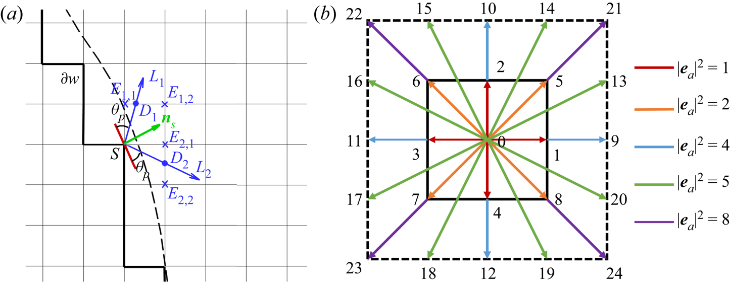
Figure 1. (a) Sketch of the geometric function scheme to achieve a prescribed contact angle  ${\theta _p}$ at the solid point S on a curved surface. (b) The D2Q25 lattice is used to calculate the unit normal vector
  ${{\boldsymbol {n}}_s}$ in (a).
In the literature, the effect of the dry air component in the implementation of contact angle is often ignored since its mass fraction is considered to be small (Zheng et al. Reference Zheng, Eimann, Philipp, Fieback and Gross2019). However, it indeed plays a role when its mass fraction is large, as in the cases considered in the following. To this aim, we suggest determining the solid density of the dry air component as
 \begin{equation} {\rho _{B,S}} = \left\{ \begin{array}{@{}ll} \min ({\rho _{B,{D_1}}},{\rho _{B,{D_2}}}), & {{}}{\theta _p} \leqslant {\rm \pi}/2,\\ \max ({\rho _{B,{D_1}}},{\rho _{B,{D_2}}}), & {{}}{\theta _p} > {\rm \pi}/2, \end{array} \right. \end{equation}
where the intersection densities  ${\rho _{B,{D_1}}}$ and
  ${\rho _{B,{D_2}}}$ are calculated using the same method described above. Such a choice is consistent with the physics that the two components have complementary wettabilities. We demonstrate in the following that the present scheme can accurately implement contact angles on curved solid walls over a wide range, independently of component mass fractions in the gas phase.
3. Model validation
In this section, we validate our proposed model in terms of three aspects: (1) ability to simulate two-component two-phase evaporation with a large dry air mass fraction in the gas phase; (2) flexibility to tune the contact angle independently of the mass fraction; and (3) capacity to reproduce a microfluidic evaporation experiment. We set  ${G_{AB}} = {G_{BA}} = 0.15$ to provide a suitable miscible state between water vapour and dry air (Zheng et al. Reference Zheng, Eimann, Philipp, Fieback and Gross2019). Following Li et al. (Reference Li, Kang, Francois, He and Luo2015), the saturation temperature is set as
  ${T_{sat}} = T/{T_{cr}} = 0.86$, and
  $a = 3/49$ and
  $b = 2/21$ are chosen, leading to saturated liquid water density
  $\rho _l^s \approx 6.5$ and water vapour density
  $\rho _v^s \approx 0.38$. The liquid vapour saturation density ratio and viscosity ratio are fixed at values of 17 and 1, respectively. Following LBM convention, lattice units are used here. We recall that the unit conversion from lattice to physical units can be conducted based on characteristic variables (Fei et al. Reference Fei, Qin, Wang, Luo, Derome and Carmeliet2022a). For convenience, components A and B are denoted as water (vapour) and air, respectively.
3.1. Achievement of large dry air mass fraction
We first validate the ability of the model to simulate two-component two-phase evaporation with a large dry air mass fraction in the gas phase. One may notice that in realistic cases, wet air is a gas mixture including nitrogen, oxygen, water vapour and other components. Here, we simplify it to be a two-component mixture (Weishaupt, Koch & Helmig Reference Weishaupt, Koch and Helmig2022) composed of water vapour and pseudocomponent dry air, since dry air, as a gas mixture, behaves similarly to its gas components taken separately and is almost insoluble in liquid water. The mass fraction of water vapour in wet air is usually below 3 % ( ${Y_{vapour}} \leqslant 3\,\%$ or
  ${Y_{air}} \geqslant 97\,\%$ ) in ambient conditions, but may vary greatly depending on environment temperature and relative humidity. In contrast, in previous lattice Boltzmann modelling, water vapour is often the main component in the gas phase and the dry air mass fraction is low, i.e. only
  ${Y_{air}} = 1\,\%$–
 $2\,\%$ for non-isothermal cases (Zheng et al. Reference Zheng, Eimann, Philipp, Fieback and Gross2019) or
  ${Y_{air}} = 10\,\%$–
 $15\,\%$ for isothermal cases (Fei et al. Reference Fei, Qin, Zhao, Derome and Carmeliet2022b). In this subsection, we first determine the maximum achievable dry air mass fraction
  ${Y_{air}}$ in our model.
The considered problem is the isothermal Stefan problem, as represented in figure 2, where the bottom and the top parts are the liquid and gas phases, respectively. Both phases are composed of two components: liquid water and a very small amount of dissolved air in the liquid phase; water vapour and dry air in the gas phase. The top boundary is open to the surrounding gas (with fixed component concentrations), and the water vapour fraction at the phase interface ( $y = 0$, subscript 1) is larger than its value at the boundary (
 $y = L$, subscript 2), i.e.
  ${Y_{vapour,1}} > {Y_{vapour,2}}$, driving the vapour diffusion from the interface to the environment, with an analytical diffusion flux (Turns Reference Turns1996)
 \begin{equation} flux = \frac{{\rho \alpha }}{L}\ln \left( {1 + {B_Y}} \right), \end{equation}
where  $L$ is the distance from the interface to the boundary and
  ${B_Y}$ is the mass transfer number defined as
  ${B_Y} = ({Y_{vapour,1}} - {Y_{vapour,2}})/(1 - {Y_{vapour,1}})$. The liquid water, therefore, evaporates to balance the mass flux due to diffusion in the gas phase, leading to the receding of the interface (increasing L). In the simulation, we vary the vapour fraction at the boundary
  ${Y_{vapour,2}}$ by changing the boundary densities (
 ${\rho _{vapour,2}}$ and
  ${\rho _{air,2}}$) simultaneously so that the total pressure p by (2.17) is kept constant. The computational domain is resolved by
  $2\Delta x \times 500\Delta x$, with periodic boundary conditions in the horizontal direction and the bounce-back scheme on the bottom boundary.
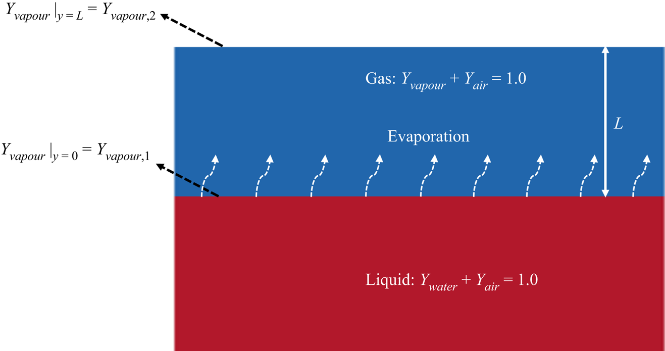
Figure 2. Schematic representation of the Stefan problem.
For the top boundary, the unknown DDFs can be approximately reconstructed based on the non-equilibrium extrapolation (NEQ) scheme (Guo, Zheng & Shi Reference Guo, Zheng and Shi2002):
 \begin{equation} \bar{f}_i^k({x_0},t) \approx \bar{f}_i^{k, \times }({x_0},t) = f_i^{k,eq}({\rho _{k,2}},{{\boldsymbol{u}}_1}) + f_i^{k,neq}({x_1},t){{}},\quad i = 4,7,8, \end{equation}
where  ${\boldsymbol {x}_0} = [ {x,L} ]$ and
  ${\boldsymbol {x}_1} = [ {x,L-1} ]$ are the boundary nodes and neighbouring fluid nodes, respectively, and
  ${\boldsymbol {u}_1}$ is the mixture velocity at
  ${\boldsymbol {x}_1}$. The viscosity is first set as
  $\nu = 0.1$ and the second-order truncated equilibrium distribution function (Qian et al. Reference Qian, d'Humières and Lallemand1992) is used to calculate
  $f_i^{k,eq}$. We first test the effect of the adjustment factor
  $\sigma$ in (2.16) by changing
  $\sigma$ progressively but fixing
  ${Y_{air,2}} = 0.24$. As shown in figure 3(a), for the case
  $\sigma =0.099$, the flux curve fluctuates significantly. With decreasing
  $\sigma$, the flux curve gradually smooths and decreases with distance
  $L$, following the trend in (3.1). Actually, by setting
  $\sigma =0.090$, for the standard single-component planar interface problem (Shan Reference Shan2008), our model reproduces thermodynamically consistent liquid–vapour coexistence densities. Therefore, such a setting is used in the following. According to the suggestion by Turns (Reference Turns1996),
  ${Y_{vapour,1}}$ is defined at the location where
  ${\rho _{vapour}} = \rho _v^s$, and for the present settings, its value is almost constant (
 ${Y_{vapour,1}} \approx 0.99$).
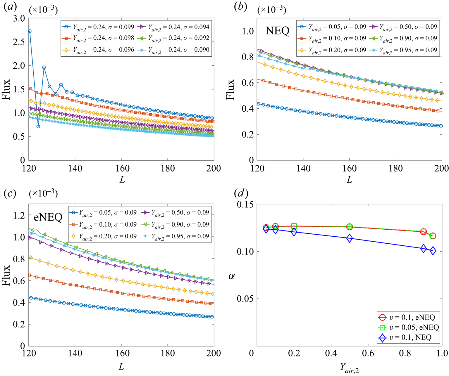
Figure 3. Simulation results of the Stefan problem. (a) Flux curves for cases with different  $\sigma$ at
  ${Y_{air,2}} = 0.24$. (b) Flux curves for cases with different
  ${Y_{air,2}}$ at
  $\sigma =0.09$ using NEQ scheme. (c) Flux curves for cases with different
  ${Y_{air,2}}$ at
  $\sigma =0.09$ using eNEQ scheme. (d) Spatially averaged binary diffusivity
  $\alpha$ for cases in (b,c), plus for
  $\nu = 0.05$ using eNEQ scheme.
According to (3.1), larger  ${Y_{air,2}}$ (corresponding to smaller
  ${Y_{vapour,2}}$ and larger mass transfer number
  ${B_Y}$) gives larger flux, which is confirmed when
  ${Y_{air,2}} \leqslant 0.5$, as seen in figure 3(b). On the contrary, when
  ${Y_{air,2}}$ is further increased, the evaporation flux begins to decrease. By carefully probing the results, it is found that, when
  ${Y_{air,2}}$ is large, the density gradient magnitude in each component
  $| {{{\partial {\rho _k}} / {\partial x}}} |$ becomes too large, leading to inaccuracy in the approximation in (3.2). More specifically, the boundary density obtained based on the NEQ scheme in (3.2) is
 \begin{equation} \rho _{k,2}^ \times{=} \sum_{i \ne 4,7,8} {\bar{f}_i^k({\boldsymbol{x}_0},t)} + \sum_{i = 4,7,8} {\bar{f}_i^{k, \times }({\boldsymbol{x}_0},t)}, \end{equation}
which deviates strongly from the value it should be, i.e.  $\rho _{k,2}$. To eliminate the mismatch,
  $\rho _{k,2}^ \times \ne {\rho _{k,2}}$, inspired by the discussion for the single-component single-phase system (Ju et al. Reference Ju, Shan, Yang and Guo2021), we propose to reconstruct the unknown DDFs at the boundary via the following exact NEQ (eNEQ) scheme:
 \begin{equation} \bar{f}_i^k({x_0},t) = \bar{f}_i^{k, \times }({x_0},t) + \beta _i^k{{}}\quad i = 4,7,8, \end{equation}
where the correction term  $\beta _i^k$ is explicitly expressed as
 \begin{equation} \beta _i^k = \frac{{w(i)}}{{\sum {w(i)} }}\left( {{\rho _{k,2}} - \rho _{k,2}^ \times } \right){{}}\quad i = 4,7,8. \end{equation}
The flux curves using the eNEQ scheme are shown in figure 3(c), and we can see that the diffusion flux can be increased by increasing  ${Y_{air,2}}$ up to 0.9. Afterward, the diffusion flux slightly decreases, as seen for the case
  ${Y_{air,2}}=0.95$. The effective binary diffusivity
  $\alpha$ can be measured by fitting the diffusion flux curves with (3.1) and the results are plotted in figure 3(d). It should be noted that the measurement of a binary diffusion coefficient based on the isothermal Stefan problem has also been validated in experiments (Slattery & Mhetar Reference Slattery and Mhetar1997). It is seen that, for the NEQ scheme, the measured
  $\alpha$ is decreasing with
  ${Y_{air,2}}$, mainly due to the above-mentioned mismatch effect. By eliminating the defect using the eNEQ scheme, the measured
  $\alpha$ is almost independent of the boundary component mass fraction at
  ${Y_{air,2}} \leqslant 0.9$, following the classical Fick's law (Turns Reference Turns1996). In addition, we also test the cases with a different mixture viscosity (
 $\nu = 0.05$), and the results are identical to
  $\nu = 0.1$ cases, indicating that the Schmidt number (
 ${S_C} = \nu /\alpha$) can be tuned in the present model. The above results confirm that our proposed model is able to simulate two-component two-phase evaporation problems with a large dry air mass fraction, up to 90 % in the gas phase.
3.2. Mass-fraction-independent contact angles
To validate the capability and accuracy of the two-component geometric function contact angle scheme introduced in § 2.3, we simulate a single droplet sitting on a curved surface with different water vapour mass fractions in the gas at different prescribed contact angles. The computational domain is a box of size  $300\Delta x \times 300\Delta x$. A solid cylinder with a radius of
  ${R_c} = 60\Delta x$ is located at
  $(150, 80)$ and a droplet with radius
  ${R_0} = 50\Delta x$ is initially placed on the cylinder with its centre at
  $(150, 180)$. The periodic boundary condition is applied in all directions, and the halfway bounce-back scheme is used to treat the solid boundary. We consider three different gas mixtures by initializing the gas phase with
  $({Y_{vapour,i}},{{}}{Y_{air,i}}) = (95\,\% ,{{}}5\,\% )$,
  $(50\,\% ,{{}}50\,\% )$ and
  $(10\,\% ,{{}}90\,\% )$, respectively. The prescribed contact angle ranges from
  ${\theta _p} = {15^ \circ }$ to
  ${\theta _p} = {135^ \circ }$.
The steady state for different cases is shown in figure 4, where the black solid line indicates the location of liquid–gas interface and the contours are for the vapour mass fraction  ${Y_{vapour}}$. Despite the different component mass fraction distributions in the gas, the droplet profiles for different
  ${Y_{vapour,i}}$ cases are essentially identical, with some very small differences at the smallest contact angle
  ${\theta _p} = {15^ \circ }$. The contact angle
  ${\theta _m}$ measured with ImageJ Fiji software for all the cases is plotted in figure 5(a), where we can see that the measured
  ${\theta _m}$ values for different
  ${Y_{vapour,i}}$ cases collapse and are consistent with
  ${\theta _p}$ values. The maximum errors are around
  $+ {3^ \circ }$ and
  $-{2^ \circ }$ at the minimum and maximum prescribed contact angles (
 ${\theta _p} = {15^ \circ }$ and
  ${\theta _p} = {135^ \circ }$), respectively. Figure 5(b) shows the maximum spurious velocity magnitude for different cases. The neutral wetting cases have smaller spurious currents compared with the hydrophilic and hydrophobic cases, and the spurious currents slightly increase for smaller vapour mass fraction. Generally, the maximum spurious current for all the cases considered is below 0.0066, which is comparable with single-component cases in the literature (Li et al. Reference Li, Yu and Luo2019). The above results confirm that our two-component contact angle implementation shows the flexibility to tune the contact angle independently of the component mass fraction and can well control the spurious currents.
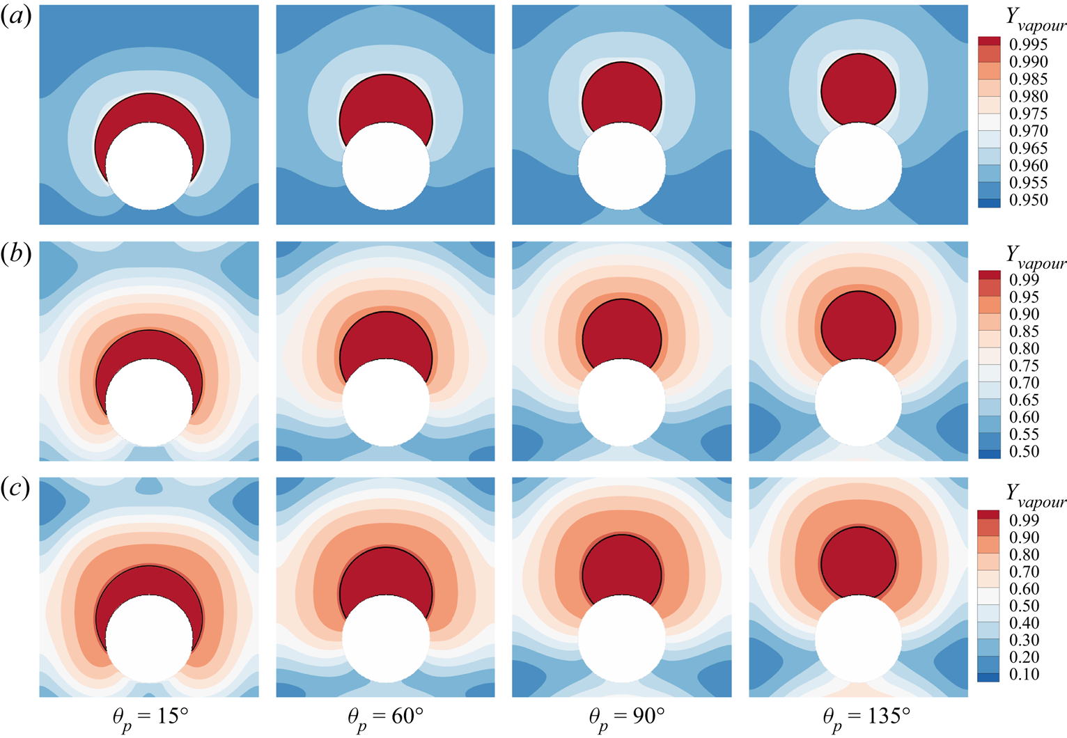
Figure 4. Validation of contact angle implementation scheme at different prescribed contact angles:  ${\theta _p} = {15^ \circ }$,
  ${\theta _p} = {60^ \circ }$,
  ${\theta _p} = {90^ \circ }$ and
  ${\theta _p} = {135^ \circ }$. Three initial water vapour mass fractions in the gas phase are considered: (a)
  ${Y_{vapour,i}}=0.95$, (b)
  ${Y_{vapour,i}}=0.5$ and (c)
  ${Y_{vapour,i}}=0.1$.
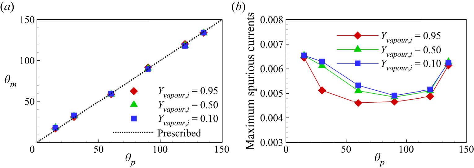
Figure 5. (a) Measured contact angles  ${\theta _m}$ versus prescribed contact angle
  ${\theta _p}$. (b) Comparison of the maximum spurious currents for different cases.
3.3. Validation with microfluidic evaporation experiment
To further validate our model for evaporation in porous media, we compare simulation results with microfluidic evaporation experimental results of Wu, Kharaghani & Tsotsas (Reference Wu, Kharaghani and Tsotsas2016). The experiment is conducted in a custom-designed network which consists of regular pores and throats. As sketched in figure 6(a), a set of  $5 \times 5$ equal-size square pores are connected by rectangular throats of different widths. The side length of the pores and the distance between centres of two neighbouring pores are fixed at
  $l = 1\ \textrm {{mm}}$ and
  $a = 2\ \textrm {mm}$, respectively. The throat widths are uniformly distributed within the range
  $0.14 \leqslant w \leqslant 0.94\ \textrm {{mm}}$, with an increment of 0.02 mm. The depth perpendicular to the plane in figure 6(a) is
  $h = 0.1\ \textrm {{mm}}$. The evaporation is driven by the vapour diffusion along the top middle pore, which is open to the environment. The contact angle of deionized water on the polydimethylsiloxane network material is about
  ${69^\circ }$. In the simulation, the network is resolved by
  $684\Delta x \times 730\Delta x$ lattices, leading to
  $11\Delta x$ for the minimum throat width. Such a resolution is recognized to be sufficiently fine for accurate lattice Boltzmann simulations of multiphase flows in porous media (Zhao et al. Reference Zhao, Qin, Derome and Carmeliet2020; Fei et al. Reference Fei, Qin, Zhao, Derome and Carmeliet2022b). A concentration boundary condition with
  $({Y_{vapour,out}},{{}}{Y_{air,out}}) = (10\,\% ,{{}}90\,\%)$ is imposed at the outlet and the halfway bounce-back scheme is applied at the solid boundary.
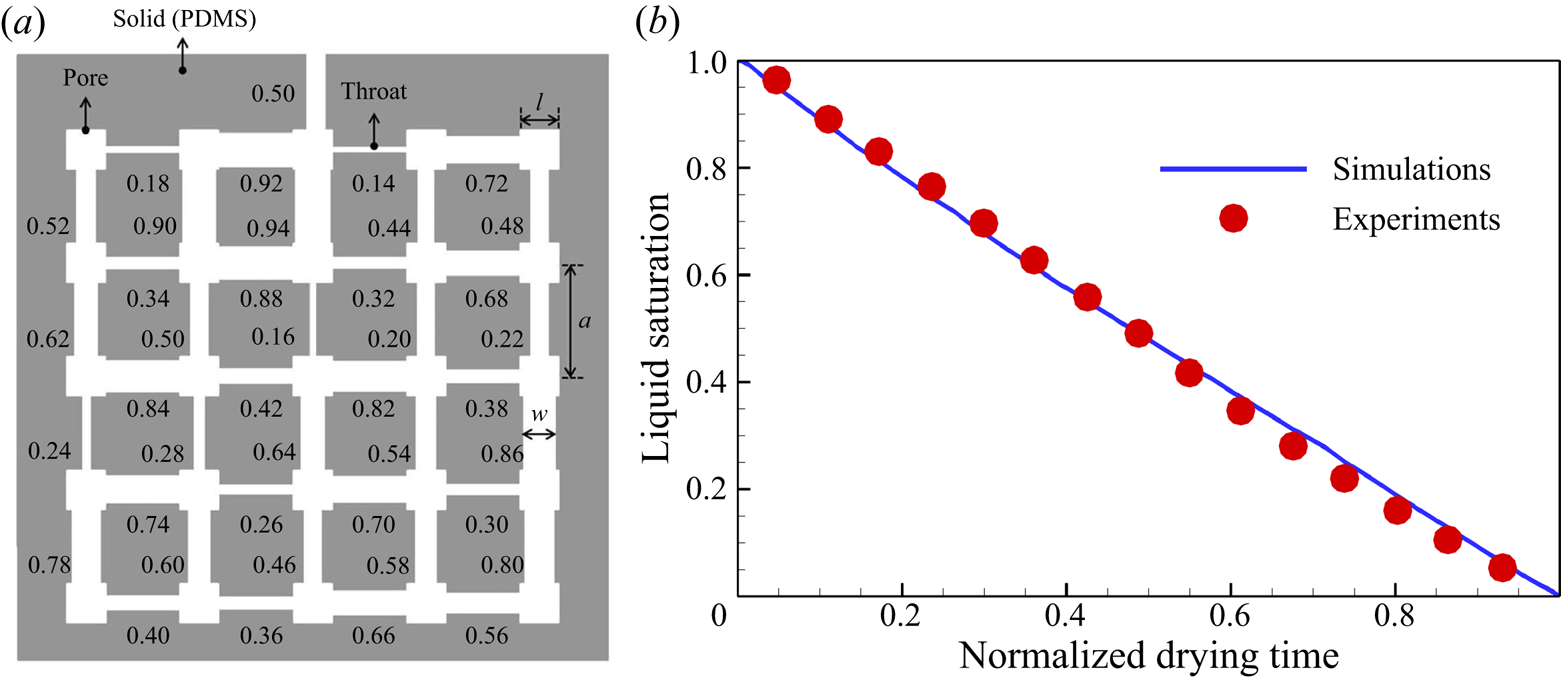
Figure 6. Validation with microfluidic evaporation experiment. (a) Structure of the network taken from Wu et al. (Reference Wu, Kharaghani and Tsotsas2016), copyright Elsevier (PDMS, polydimethylsiloxane). (b) Variation of the liquid saturation with drying time normalized by the total drying time.
As shown in figure 6(b), the normalized time evolution of the liquid saturation by our simulation coincides with the experiment results. Saturation decreases almost linearly with time in both simulation and experiment, indicating evaporation undergoes a constant rate period (CRP). As further illustration, the liquid distribution in the network at different liquid saturations S is presented in figure 7, showing that the top right corner remains filled with liquid until the end and therefore that the evaporation regime remains in CRP. For different liquid saturation values, the liquid distributions by our simulation are well consistent with the experiment, despite some minor differences. Some residual liquid patches are seen in simulation, but not in experiment. At  $S = 0.49$, the left top corner is dried out in simulation while it is still filled with liquid in experiment. One of the reasons for the small differences is that the simulations are carried out in two dimensions, but the experiments are conducted in three dimensions, as analysed by Liu et al. (Reference Liu, Sun, Wu, Wei and Hou2021). In Appendix B, a preliminary 3-D simulation is conducted using the 3-D multiphase CLBM (Fei et al. Reference Fei, Yang, Chen, Mo and Luo2020). Compared with the current 2-D simulation, the main liquid configuration remains the same, indicating the acceptable accuracy of the 2-D simulation. The improvement of 3-D simulation lies in that the isolated liquid patches almost disappear, as shown in figure 20. In addition, leaving out contact angle hysteresis in the proposed algorithm may also result in some differences (Xu, Liu & Valocchi Reference Xu, Liu and Valocchi2017). Generally, the accuracy of the present simulation is within an acceptable range.
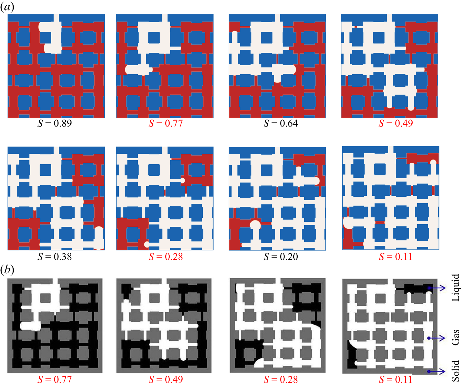
Figure 7. Evolution of the liquid distribution in the network at different liquid saturations S. (a) The LBM simulations in the present work. (b) Experimental images taken from Wu et al. (Reference Wu, Kharaghani and Tsotsas2016), copyright Elsevier.
4. Numerical results and discussion
4.1. Simulation set-up
In this section, the model proposed above is applied to study convective evaporation in a synthetic porous medium. The porous medium is designed with a dual-porosity geometry by filling a rectangular domain ( $L \times H = 481\Delta x \times 401\Delta x$) with larger solid cylinders on both sides and smaller cylinders in its middle region, leading to porosities of
  ${\phi _1} \approx 0.64$ and
  ${\phi _1} \approx 0.82$ in each region, respectively. The mean porosity is
  $\bar {\phi }\approx 0.72$. Such dual-porosity configuration is retained to mimic the capillary pumping effect induced by the heterogeneous pore structures in real porous media, an approach similarly applied in the literature (Qin et al. Reference Qin, Del Carro, Mazloomi Moqaddam, Kang, Brunschwiler, Derome and Carmeliet2019, Reference Qin, Zhao, Kang, Derome and Carmeliet2021; Gu, Liu & Wu Reference Gu, Liu and Wu2021). To ensure numerical accuracy, the smallest cylinder diameter is set as
  ${D_m} = 15\Delta x$, which is three times the interface thickness showing the resolution needed for pore-scale simulations (Zhao et al. Reference Zhao, Qin, Derome and Carmeliet2020; Fei et al. Reference Fei, Qin, Zhao, Derome and Carmeliet2022b). The porous medium is installed in the middle bottom of the computational domain and initially filled with liquid water, as sketched in figure 8(a). Its top surface is exposed to a gas mixture that is blowing over it with a Poiseuille inflow (with peak velocity
  ${U_m} = 0.08$), purging the vapour by convection and diffusion. The channel height
  ${H_1}$ is chosen to be large enough to resolve the fully developed vapour boundary layer thickness. For a free-stream flow over an impermeable flat plate, the vapour boundary layer thickness can be approximated by the following expression (Leal Reference Leal1992):
 \begin{equation} {\delta _m} = \delta S{c^{ - 1/3}} \approx 4.64X{Re} _x^{ - 1/2}{\left( {{\nu / \alpha }} \right)^{ - 1/3}}. \end{equation}
Here  $\delta$ is the momentum boundary layer thickness and
  ${{Re}_x} = {U_\infty }X/\nu$ is the local Reynolds number defined based on the downstream location
  $X$ and the free-stream gas velocity. For our cases, the boundary layer is affected by two other factors: the top surface of the porous medium (
 ${y=H}$) is permeable and its vapour concentration is non-uniform and variable. For a typical case, the vapour boundary layer thickness profile follows (4.1) in the beginning at the upstream, and gradually decreases with time, as shown in figure 8(b). To resolve the boundary layer, the channel height is chosen as
  ${H_1} = 100\Delta x$, leading to an inflow Reynolds number
  ${Re} = {U_m}{H_1}/2\nu = 100$ with
  $\nu = 0.04$. Based on preliminary tests, we set the inlet section length
  ${L_1} = {H_1}$ and the outlet section length
  ${L_2} = 2{H_1}$ to eliminate inlet/outlet effects.
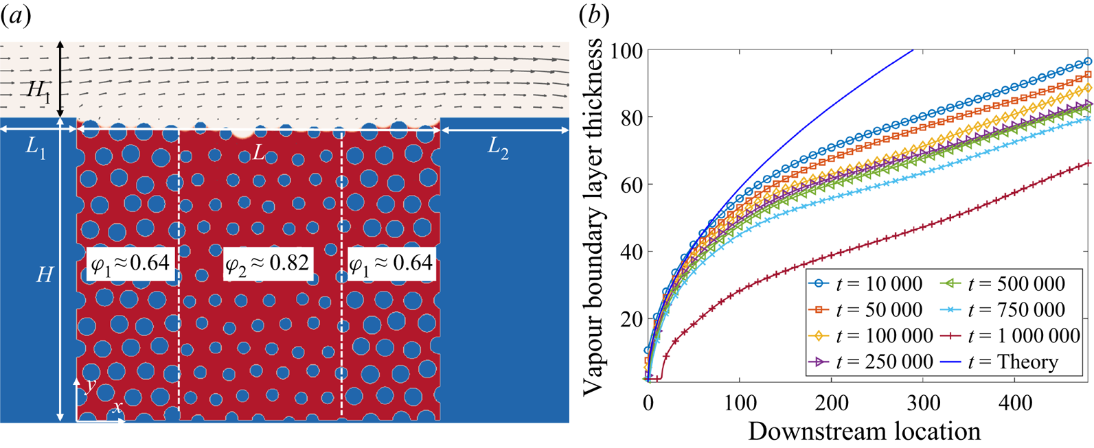
Figure 8. (a) Simulation set-up. A dual-porosity medium filled with liquid water is installed in the middle bottom. A mixture gas (dry air  $+$ water vapour) is convectively blown in the top channel, with a Poiseuille inflow velocity profile. (b) Development of vapour boundary layer thickness for a typical case. The solid line is the Blasius solution.
In the simulations, the convective boundary condition (Lou, Guo & Shi Reference Lou, Guo and Shi2013) is imposed at the outlet and the halfway bounce-back scheme is applied to deal with the non-slip boundary conditions at the channel walls and the porous medium solid matrix. The flexibility of the present model makes it possible to conduct a systematic parametric study of evaporation in porous media at the pore scale. To highlight this, we probe the effects of two key parameters, inflow vapour concentration  ${Y_{vapour,in}}$ and contact angle
  $\theta$, on the evaporation dynamics. To study the effect of inflow vapour concentration, we first fix the contact angle and vary
  ${Y_{vapour,in}}$ from 0.95 to 0.1 (marked as Group 1 in table 1). Similarly, we then consider the effect of contact angle by fixing the inflow vapour concentration while changing
  $\theta$ from
  ${15^ \circ }$ to
  ${105^ \circ }$ (marked as Group 2). It may be noted that the capillary pumping effect plays a role for hydrophilic conditions, and therefore we mainly consider cases with
  $\theta \leqslant {90^ \circ }$. An additional contact angle
  $\theta = {105^ \circ }$ is also included to show the evaporation patterns for slightly hydrophobic conditions. In addition, we consider another six cases (marked as Group 3) for completeness of our considered parametric space. The considered cases spread within a wide range of the parameters, i.e.
  $0.1 \leqslant {Y_{vapour,in}} \leqslant 0.98$ and
  ${15^ \circ } \leqslant \theta \leqslant {105^ \circ }$, as summarized in table 1.
Table 1. Cases considered for the effect of contact angle ( $\theta$) and inflow vapour concentration (
 ${Y_{vapour,in}}$).
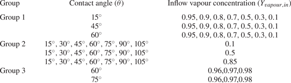
4.2. Effect of inflow vapour concentration  ${Y_{vapour,in}}$

The snapshots of the convective evaporation with  $\theta = {15^ \circ }$ and three typical inflow vapour concentration cases,
  ${Y_{vapour,in}} = 0.9$, 0.5 and 0.1, are presented in figure 9 (see also supplementary movies 1, 2 and 3 available at https://doi.org/10.1017/jfm.2022.1048). For each case, it is clearly shown that the liquid–gas interface (indicated by the solid black line) recedes first from the middle region. When the middle region is almost completely dried, the evaporation front starts to recede in the side regions. Such behaviour is directly attributed to the capillary pumping effect. The capillary pressure
  ${p_c}$, defined based on the surface tension
  $\gamma$ and the radius of curvature in the local pores
  $r$ by
  ${p_c} = \gamma \cos (\theta )/r$, is larger in the smaller pores on both side regions than that in the middle larger pores. Since in our case the mixture gas in the channel is open to the environment and kept at constant gas pressure
  ${p_g}$, the liquid pressure (
 ${p_l} = {p_g} - {p_c}$) is higher in the middle region than that in side regions. Such a liquid pressure difference keeps pumping the liquid from the larger pores to the smaller pores, leading to the evaporation front receding in the middle but remaining pinned at the channel level in the side regions. As the middle region dries, the evaporation front gradually penetrates deeper and finally percolates through the porous medium, e.g.
  $t = 1.0 \times {10^6}$ in figure 9(a), then the capillary pumping effect is weakened and can no longer supply sufficient liquid to the smaller pores. Afterward, the evaporation begins to recede in the side parts, showing a decrease in the global evaporation rate. By decreasing the inflow vapour concentration from
  ${Y_{vapour,in}} = 0.9$ to
  ${Y_{vapour,in}} = 0.5$, the evaporation rate is significantly increased up to
  $t = 1.0 \times {10^6}$, as evidenced by the difference in the penetration depths and dried out structures. The global drying curves for different cases are discussed later in figure 11. It is as expected because the main evaporation driving force, i.e. vapour concentration gradient from the channel to the liquid–vapour interface, is larger in figure 9(b) than in figure 9(a). By further decreasing
  ${Y_{vapour,in}}$ to 0.1, the evaporation rate can be further increased but not so remarkably, as seen in figure 9(c).
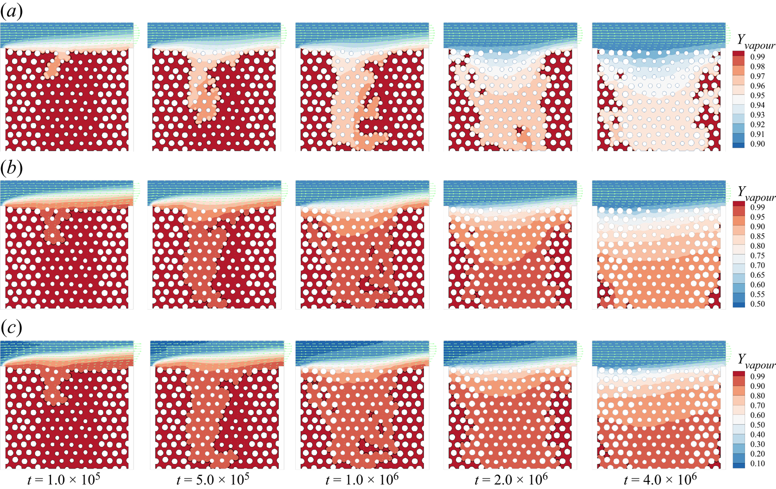
Figure 9. Time evolution of liquid distribution in the porous medium for cases with  $\theta = {15^ \circ }$. The arrows show the velocity field, the solid black lines indicate the liquid–gas interface locations and the contours present the vapour mass fraction: (a)
  ${Y_{vapour,in}} = 0.9$ (supplementary movie 1), (b)
  ${Y_{vapour,in}} = 0.5$ (supplementary movie 2) and (c)
  ${Y_{vapour,in}} = 0.1$ (supplementary movie 3).
Benefiting from the present pore-scale model, we can quantify the local degrees of evaporation by explicitly obtaining the pore-scale information from our simulation results. We first consider the vertical profiles of saturation,  ${S_y}$, defined as the ratio of pore cells occupied by liquid phase to the total pore cells at a certain height
  $y$. The time evolution of the saturation profiles for the case with
  $\theta = {15^ \circ }$ and
  ${Y_{vapour,in}} = 0.9$ is plotted in figure 10(a). At the very beginning (
 $t = 1.0 \times {10^4}$), the porous medium is almost fully filled, showing a step change from
  ${S_y} = 1.0$ to 0 close to
  $y = H$. With ongoing time, the profiles are gradually smoothed out by widening the unsaturated zone (
 $0 < {S_y} < 1.0$) and thinning the fully filled zone (
 ${S_y} = 1.0$). At
  $t = 1.0 \times {10^6}$, the fully filled zone disappears as the evaporation front in the middle region has reached the bottom, seen also in figure 9(a). The vertical saturation profiles then decrease entirely, but very slowly due to the decreased evaporation rate mentioned above. For the cases with different
  ${Y_{vapour,in}}$, the time evolution of
  ${S_y}$ profiles has the same trend, as seen, for example, in figure 10(b) for
  ${Y_{vapour,in}} = 0.1$. Compared with figure 10(a), the major difference is that the fully filled zone disappears earlier at
  $t = 5.0 \times {10^5}$ due to its larger evaporation rate. Figures 10(c) and 10(d) show the local evaporation rates at the top surface of the porous medium, corresponding to figures 10(a) and 10(b), respectively. Initially, the evaporation is strongest at the leftmost throat, where the inflowing gas mixture is at the lowest vapour concentration
  ${Y_{vapour}}$, and continues to decrease along the downstream direction as the gas mixture gets more and more saturated with water vapour. The evaporation rate at the left throats decreases dramatically from
  $t = 1.0 \times {10^6}$ to
  $t = 2.0 \times {10^6}$ in figure 10(c) (similarly, from
  $t = 7.5 \times {10^5}$ to
  $t = 1.0 \times {10^6}$ in figure 10d), since the capillary pumping effect is no longer at play and the evaporation front begins to recede in the side regions. However, the evaporation rate at the rightmost throat remains almost unchanged, mainly because the convective flow enters the porous medium, flows parallel to the surface, continues to accumulate vapour and exits again at the rightmost throat. As a result, we can see a clear pattern transition, from left–high–right–low to left–low–right–high, in both figures 10(c) and 10(d), which is consistent with the convective evaporation dynamics in a homogeneous porous medium reported by Weishaupt & Helmig (Reference Weishaupt and Helmig2021).
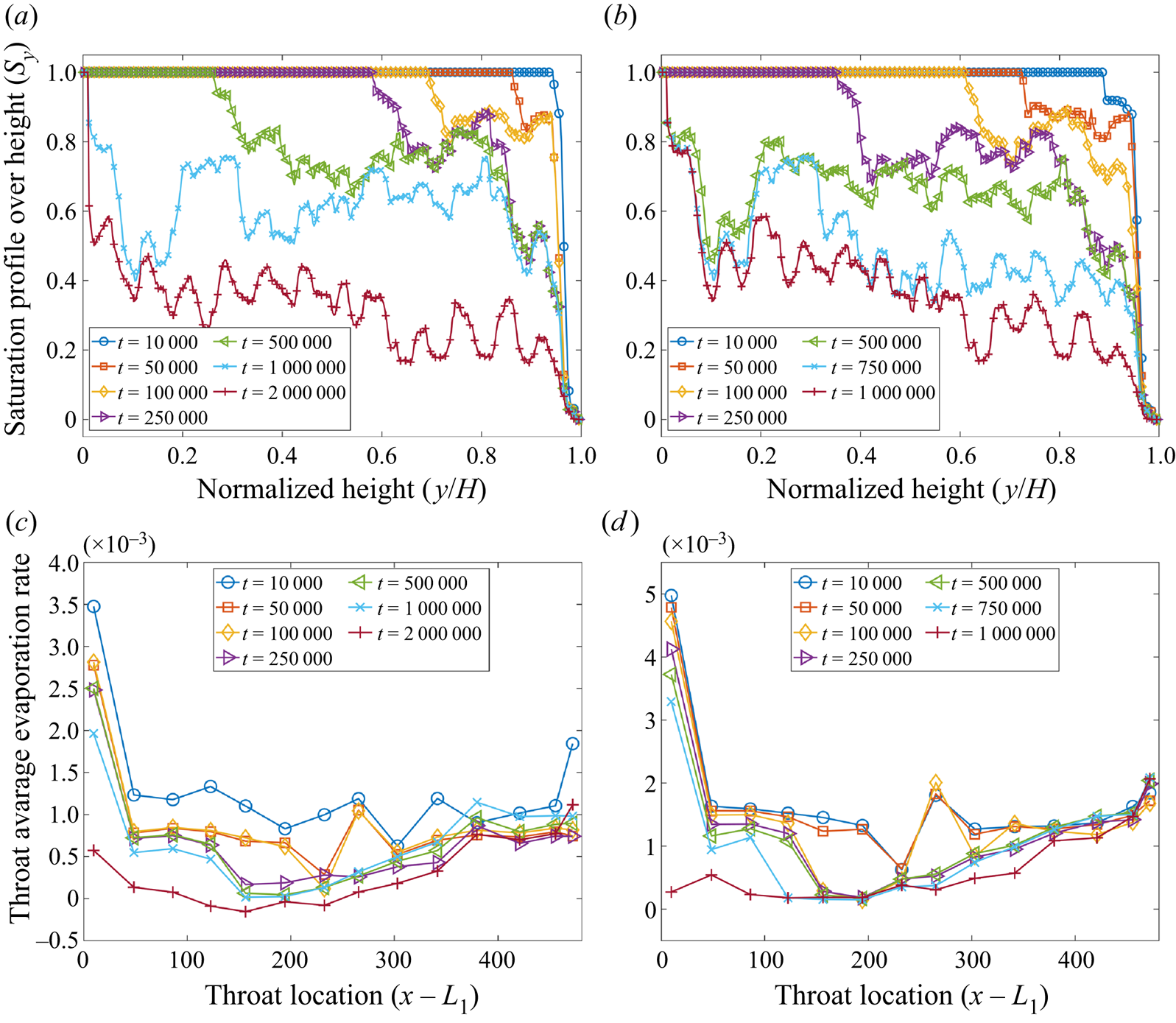
Figure 10. Pore-scale evaporation behaviours. Saturation profiles over height ( ${S_y}$) for cases with (a)
  ${Y_{vapour,in}} = 0.9$ and (b)
  ${Y_{vapour,in}} = 0.1$. Pore-local evaporation rates at the top surface of the porous medium (
 $y = H$) for (c)
  ${Y_{vapour,in}} = 0.9$ and (d)
  ${Y_{vapour,in}} = 0.1$.
To probe the global evaporation dynamics, the time evolution of the residual liquid mass for the cases with  $\theta = {15^ \circ }$ is shown in figure 11(a). It can be seen that, with the decrease of
  ${Y_{vapour,in}}$, the residual liquid mass drops faster, because a larger concentration difference leads to a larger evaporation rate. For each case, the slope of the curve is steeper in the early stage but flattens in later stages. The completion of the evaporation takes a very long time, so our simulations are stopped when the global saturation
  $S < 0.1$ for all cases (except for the slowest case
  ${Y_{vapour,in}} = 0.95$). For a better understanding of the cause of the change in these curve slopes, we plot the data as drying curves, i.e. evaporation rate versus mean liquid saturation, in figure 11(b). For classical drying curves of porous media, three main periods have been widely identified (Chauvet et al. Reference Chauvet, Duru, Geoffroy and Prat2009). In the first period, referred to as the CRP, the evaporation rate is essentially constant. The last period is the receding front period (RFP), characterized by a significant evaporation front receding into the porous medium, whereas the transition period, the falling rate period (FRP), is an intermediate crossover period characterized by a fast drop in the evaporation rate. Figure 11(b) shows that our present model well captures the three typical evaporation periods. We emphasize that the evaporation rate in the CRP is not actually constant (Coussot Reference Coussot2000) and a slightly decreasing trend similar to our cases is often seen (Chauvet et al. Reference Chauvet, Duru, Geoffroy and Prat2009). It is non-trivial to define strict boundaries between the three periods. For our cases, the CRP is sustained by continuously supplying liquid water to the smaller pores via capillary pumping. Since the pore volume of the middle pores makes up approximately half of the total pore volume, we define the CRP as the evaporation period at
  $S > 0.5$. The FRP is defined between
  $S=0.5$ and
  $S=0.25$ as the evaporation rate is significantly decreased within this range. For other cases in Group 1, i.e.
  ${Y_{vapour,in}} = [0.95,0.9,0.8,0.7,0.5,0.3,0.1]$ at
  $\theta = {45^ \circ }$ and
  $\theta = {60^ \circ }$, the evaporation curves are similar and we can also observe the three main periods, as shown in figures 11(c) and 11(d). It is also seen that, with increasing contact angle, the transition from CRP to RFP is smoothed out because the capillary pumping effect is gradually weakened.

Figure 11. Global evaporation behaviours. (a) Time evolution of the residual liquid mass for cases with  $\theta = {15^ \circ }$. Evaporation curves (evaporation rate versus mean liquid saturation) for cases with
  $\theta =$ (b)
  ${15^ \circ }$, (c)
  ${45^ \circ }$ and (d)
  ${60^ \circ }$.
From figure 11(b–d), we can see that the evaporation rate increases with decreasing  ${Y_{vapour,in}}$, i.e. increasing inflow dry air mass fraction
  ${Y_{air,in}}$, thus approaching common conditions. To quantify this dependence, we plot the average evaporation rate in the CRP (
 $E{R_{CRP}}$) versus
  ${Y_{vapour,in}}$ at different contact angles in figure 12(a). We observe that, at a given
  ${Y_{vapour,in}}$,
  $E{R_{CRP}}$ is larger for the smaller-contact-angle case due to its significantly stronger capillary pumping effect. Moreover, at each contact angle,
  $E{R_{CRP}}$ increases nonlinearly with decreasing
  ${Y_{vapour,in}}$. To interpret the underlying mechanism, we refer again to the Stefan evaporation model introduced in § 3.1. As shown in (3.1), for the pure diffusion evaporation, the evaporation rate is proportional to
  $\ln (1 + {B_Y})$ rather than to the vapour concentration difference. In our present cases, the mass transfer number
  ${B_Y}$ can straightforwardly be defined based on the vapour concentration at the liquid–gas interface (
 ${Y_{vapour,1}}$) and the inlet (
 ${Y_{vapour,in}}$) by
  ${B_Y} = ({Y_{vapour,1}} - {Y_{vapour,in}})/(1 - {Y_{vapour,1}})$. The dependence of
  $E{R_{CRP}}$ on
  $(1 + {B_Y})$ is plotted on a semi-log scale in figure 12(b). The linear fitting for all three contact angle configurations confirms the log-law scaling dependence:
 \begin{equation} E{R_{CRP}} \propto \ln ({B_Y} + 1). \end{equation}
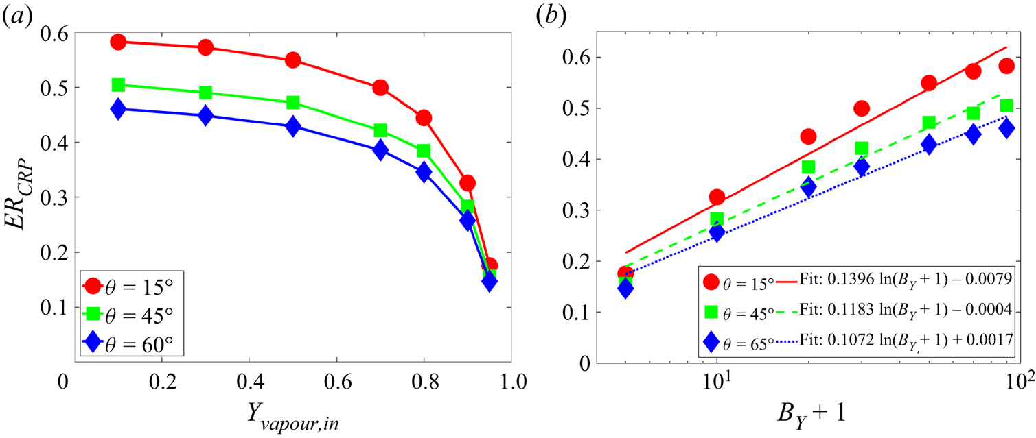
Figure 12. (a) Dependence of the average evaporation rate in CRP ( $E{R_{CRP}}$) on inflow vapour concentration (
 ${Y_{vapour,in}}$). (b) Dependence of
  $E{R_{CRP}}$ on the mass transfer number
  ${B_Y} = ({Y_{vapour,1}} - {Y_{vapour,in}})/(1 - {Y_{vapour,1}})$. The plot is on a semi-log scale.
Further, with ongoing evaporation, the liquid saturation decreases to be small enough and the system goes into the RFP. In this period, the evaporation rate does not increase significantly with decreasing  ${Y_{vapour,in}}$, as seen in figure 11(b–d). Actually, when the liquid saturation is small enough (
 $S=0.2$), the evaporation front has receded deeply into the porous medium. At such a stage, the vapour concentration profile inside the porous medium changes slightly, although the inflow vapour concentration varies largely, as seen in figure 13(a). It is found that the log-law scaling in (4.1) still works for the average evaporation rate in RFP (
 $E{R_{RFP}}$) but with a smaller prefactor than in CRP, as shown in figure 13(b). Contrary to
  $E{R_{CRP}}$,
  $E{R_{RFP}}$ is larger for the larger-contact-angle case. These different effects of contact angle on CRP and RFP are analysed in the next subsection.
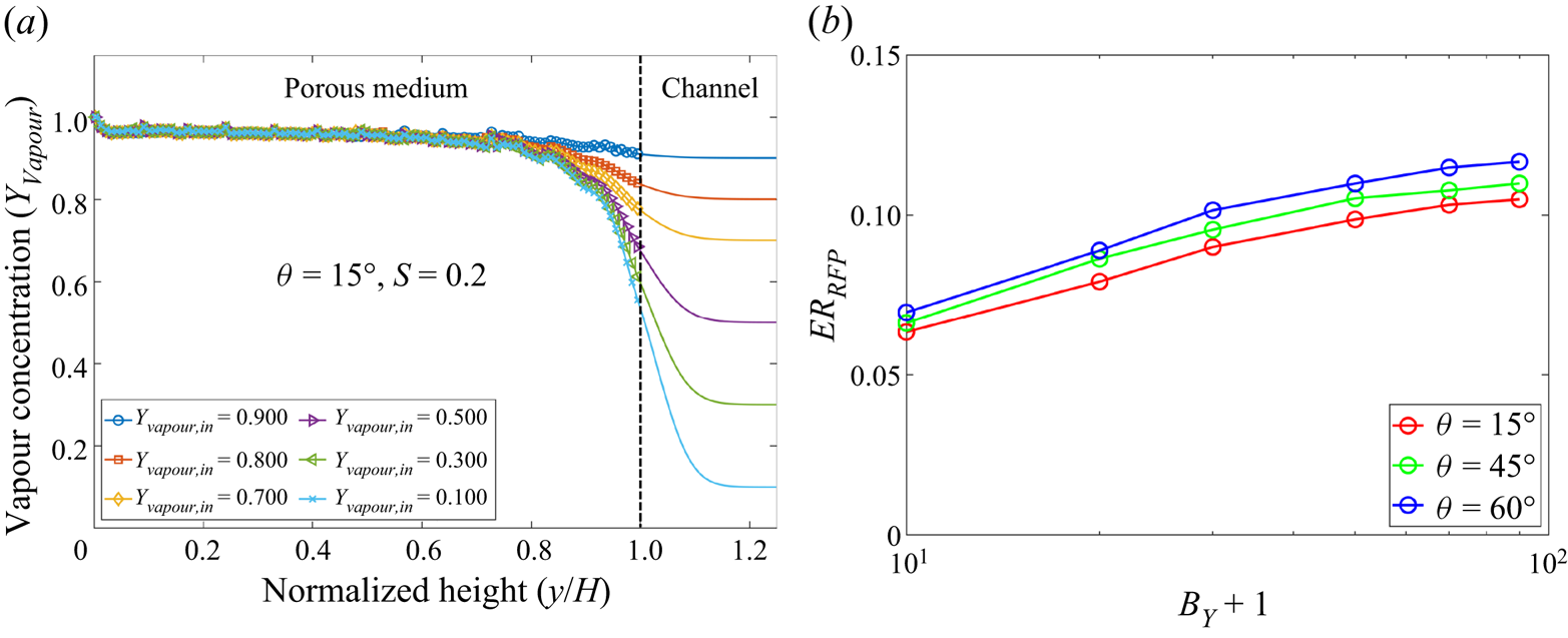
Figure 13. (a) Comparison of the vapour concentration profiles for different cases with  $\theta = {15^ \circ }$ at
  $S=0.2$. (b) Dependence of the average evaporation rate in RFP (
 $E{R_{RFP}}$) on the mass transfer number
  ${B_Y}$ for different contact angles. The plot is on a semi-log scale.
4.3. Effect of contact angle $\theta$

To study the effect of contact angle on the evaporation dynamics, we vary the contact angle  $\theta$ at a fixed inflow vapour concentration. The time evolution of the liquid distribution in the porous medium for different contact angles
  $\theta = {30^ \circ }$,
  $\theta = {60^ \circ }$ and
  $\theta = {105^ \circ }$ is shown in figures 14(a)–14(c), respectively (see also supplementary movies 4, 5 and 6). For all cases, we see that the evaporation front recedes first in the middle and then in the side regions, similar to figure 9. As we have discussed, for the hydrophilic cases, the capillary pumping effect leads to such an evaporation pattern. For a larger contact angle, the capillary pumping is less significant. As a result, the case with
  $\theta = {60^ \circ }$ evaporates slower than the
  $\theta = {30^ \circ }$ case, as evidenced at
  $t = 1.0 \times {10^6}$ that the evaporation front has penetrated through the middle large pores for
  $\theta = {30^ \circ }$ in figure 14(a) but not yet for
  $\theta = {60^ \circ }$ in figure 14(b). For the weak hydrophobic case
  $\theta = {105^ \circ }$, the capillary pressure
  ${p_c} = \gamma \cos (\theta )/r$ is negative. Therefore, the liquid pressure in the smaller pores is larger than that in the larger pores, leading to weak pumping flow from the side parts to the middle part, explaining why the evaporation front recedes from the beginning (
 $t = 1.0 \times {10^5}$) over the total surface. For the larger pores, although liquid is partially supplied from smaller pores, the evaporation front still recedes faster because they show wider vapour diffusion pathways (larger vapour permeability). Nevertheless, the competing effects of the above two phenomena result in a more compact evaporation pattern, and therefore it takes much longer for the evaporation front to completely penetrate through the middle part, as seen in figure 14(c). In addition, at a smaller contact angle, the liquid–vapour interface is more curved together with more isolated liquid islands, and its length is longer (as also seen in the supplementary movies), which helps to increase evaporation since the evaporation rate is generally proportional to the area of the liquid–vapour interface (Qin et al. Reference Qin, Del Carro, Mazloomi Moqaddam, Kang, Brunschwiler, Derome and Carmeliet2019).
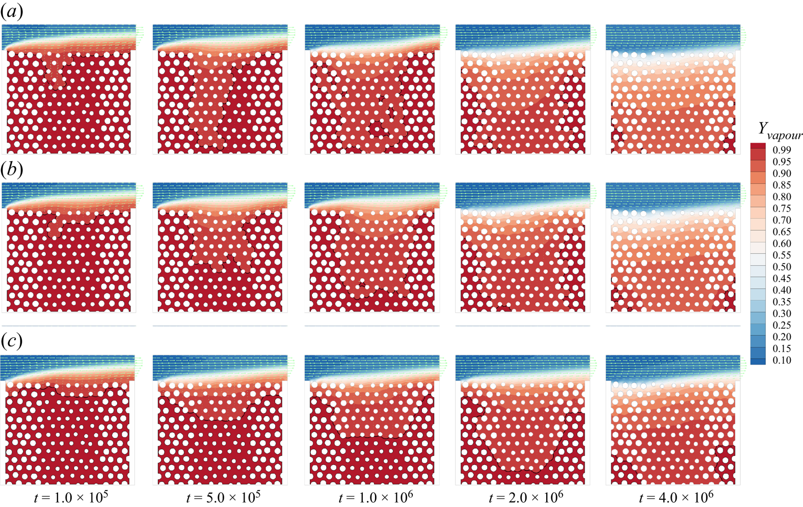
Figure 14. Time evolution of the liquid distribution in the porous medium for cases with  ${Y_{vapour,in}} = 0.1$. The arrows show the velocity field, the solid black lines indicate the liquid–gas interface locations and the contours are for the vapour mass fraction distributions. Contact angle (a)
  $\theta = {30^ \circ }$ (supplementary movie 4), (b)
  $\theta = {60^ \circ }$ (supplementary movie 5) and (c)
  $\theta = {105^ \circ }$ (supplementary movie 6).
In terms of the global evaporation behaviour, the time evolution of the residual liquid mass for the cases with  ${Y_{vapour,in}} = 0.1$ and different
  $\theta$ is shown in figure 15(a). The liquid mass decreases faster for smaller
  $\theta$, mainly due to its more significant capillary pumping effect. For all cases (except for
  $\theta = {105^ \circ }$), we can see a clear phase transition, from a fast evaporation stage in the beginning to a slow evaporation stage in the end, experiencing different evaporation periods. The corresponding evaporation curve is shown in figure 15(b). It is clearly shown that for most of the cases, the evaporation goes through a CRP at large saturation levels, followed by a fast FRP and finally enters into the RFP. At smaller contact angles (
 $\theta \leqslant {45^ \circ }$), the CRP is well sustained by the sufficient liquid supply pumped from the larger pores, as evidenced by the plateaus in figure 15(b–d). When
  $\theta$ increases, the pumping effect weakens not providing sufficient liquid supply leading to a slightly decreasing evaporation rate in drying curves at
  $S \geqslant 0.5$. For the weak hydrophobic case (
 $\theta = {105^ \circ }$), the evaporation rate keeps decreasing, and thus a CRP cannot be identified. To be consistent throughout the paper, the region
  $S \geqslant 0.5$ is identified as CRP although the transition point from CRP to FRP occurs at a higher degree of saturation for the higher contact angles. Such results are consistent with figure 14(c) showing that the evaporation front keeps receding in both large and small pores, never being pinned at the surface throughout the entire evaporation process. Similar to figure 15(b), the evaporation curves for cases of intermediate and large inflow vapour concentration (
 ${Y_{vapour,in}} = 0.5$ and 0.85) experience the three typical evaporation periods, as seen in figures 15(c) and 15(d).

Figure 15. Global evaporation behaviour. (a) Time evolution of the residual liquid mass for cases with  ${Y_{vapour,in}} = 0.1$ and different contact angles
  $\theta$. Evaporation curves for cases with
  ${Y_{vapour,in}} =$ (b) 0.1, (c) 0.5 and (d) 0.85.
To study the quantitative effect of the contact angle on the evaporation rate, we plot the average evaporation rate in CRP ( $E{R_{CRP}}$) versus
  $\theta$ for all the Group 2 cases in table 1 in figure 16(a). Generally,
  $E{R_{CRP}}$ decreases with
  $\theta$ and at given
  $\theta$ a larger
  $E{R_{CRP}}$ is seen at smaller
  ${Y_{vapour,in}}$. In our cases, CRP occurs due to the significant capillary pumping flow from larger to smaller pores (or the opposite in the slightly hydrophobic case). Therefore, one may expect that
  $E{R_{CRP}}$ depends on
  $\cos (\theta )$. As shown in figure 16(b), very good linear relations are found between
  $E{R_{CRP}}$ and
  $\cos (\theta )$,
 \begin{equation} E{R_{CRP}} \propto \cos (\theta ), \end{equation}
which confirms that the capillary pumping effect is dominant in the CRP for the present considered cases.
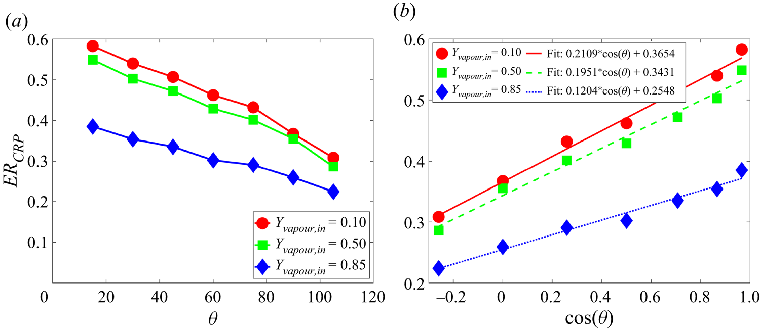
Figure 16. (a) Dependence of average evaporation rate in CRP ( $E{R_{CRP}}$) on contact angle (
 $\theta$). (b) Dependence of
  $E{R_{CRP}}$ on
  $\cos (\theta )$.
In contrast, it is interesting to see from figure 15(b–d) that in the RFP, the larger contact angle leads to a higher evaporation rate, especially for large  ${Y_{vapour,in}}$ in figure 15(d), as also seen in the results of figure 13(b). Such an opposite dependence of evaporation rate in the RFP on the contact angle is related to the Kelvin effect. The Kelvin effect refers to the change in vapour pressure above a curved interface by the following expression (Maalal, Prat & Lasseux Reference Maalal, Prat and Lasseux2021):
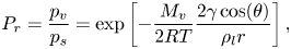 \begin{equation} {P_r} = \frac{{{p_v}}}{{{p_s}}} = \exp \left[ { - \frac{{{M_v}}}{{2RT}}\frac{{2\gamma \cos (\theta )}}{{{\rho _l}r}}} \right], \end{equation}
where  ${P_r}$ is the normalized vapour pressure (or relative humidity) and
  ${M_v}$ is the vapour molecular weight. Figure 17 shows the normalized vapour pressure distributions for three different contact angle cases at a liquid saturation
  $S = 0.2$. The larger the contact angle, the larger the vapour pressure near the liquid–gas interface, which is qualitatively consistent with (4.4). Thus, the vapour concentration inside the porous medium is higher at a larger contact angle, as shown in figure 18(a). Since the inlet vapour concentration in the channel is fixed by
  ${Y_{vapour,in}}$, the larger concentration gradient for the larger-contact-angle case leads to a higher evaporation rate. If such an effect is dominant, one could expect the logarithm of
  $E{R_{RFP}}$ to decrease linearly with
  $\cos (\theta )$. As seen in figure 18(b), generally, the linear relation
  $\ln (E{R_{RFP}}) \propto - \cos (\theta )$ works well, although some deviations can be observed. Actually, the concentration difference due to the Kelvin effect is not large, reaching only several per cent at most. If the vapour concentration in the channel is large, such a concentration difference inside the porous medium will have a marked effect and therefore the trend for
  ${Y_{vapour,in}} = 0.85$ follows better the linearly decreasing scaling. One may also notice that, for
  $\theta = {105^ \circ }$, the evaporation front seen in figure 14(c) is very compact, leading to a longer diffusion length from the liquid–gas interface to the channel than other cases, which counters the advantage procured by the Kelvin effect and may explain the local decrease of
  $E{R_{RFP}}$ for the
  ${Y_{vapour,in}} = 0.1$ curve at
  $\theta = {105^ \circ }$.
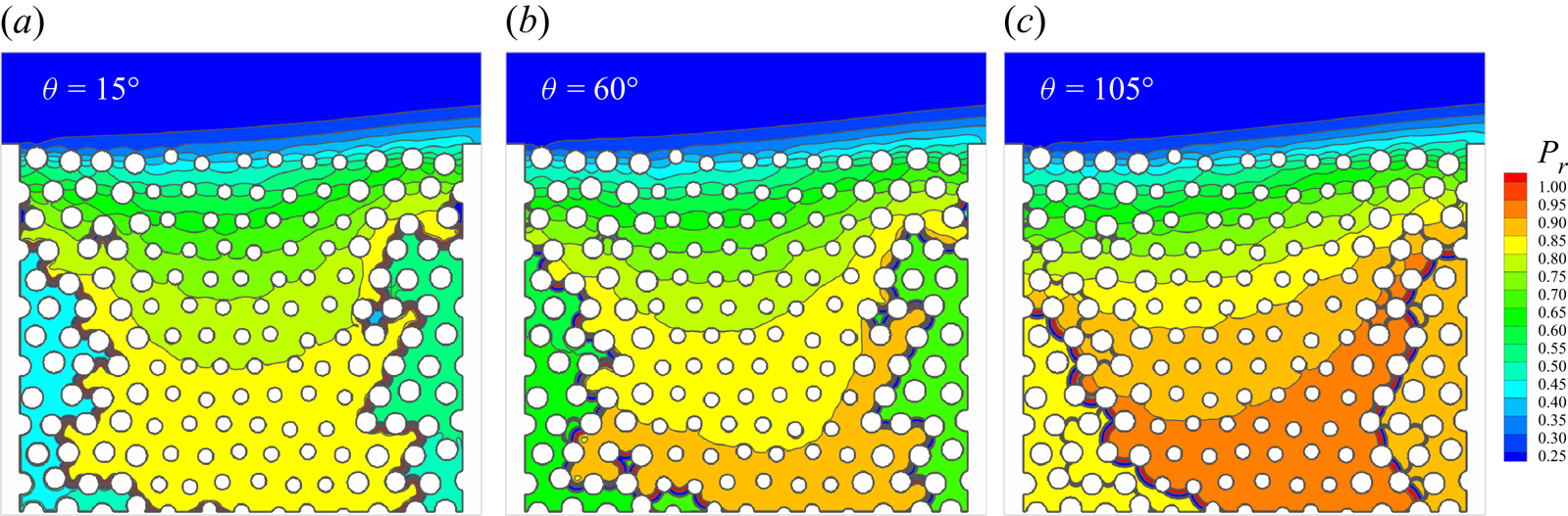
Figure 17. Normalized vapour pressure distribution with  ${Y_{vapour,in}} = 0.5$ at
  $S = 0.2$ for different contact angles: (a)
  $\theta = {15^ \circ }$, (b)
  $\theta = {60^ \circ }$ and (c)
  $\theta = {105^ \circ }$.
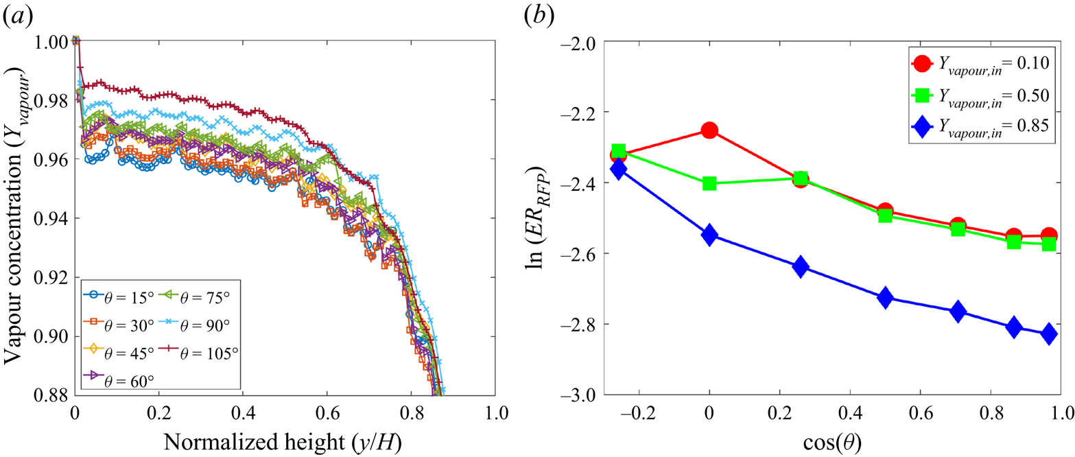
Figure 18. (a) Comparison of the vapour concentration profiles for different cases with  ${Y_{vapour,in}} = 0.5$ at
  $S = 0.2$. (b) Average evaporation rate in RFP (
 $E{R_{RFP}}$) versus
  $\cos (\theta )$.
4.4. Universal scaling relation in CRP
Up to now, we have discussed that the evaporation rate in the CRP increases on decreasing the inflow vapour concentration  ${Y_{vapour,in}}$ and the contact angle
  $\theta$ distinctly. Two scaling relations for the two parameters have been found, i.e. (4.2) and (4.3), respectively. In addition, we have also shown that the inflow Reynolds number (Re) affects the evaporation rate in the CRP by the following scaling (Fei et al. Reference Fei, Qin, Zhao, Derome and Carmeliet2022b):
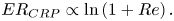 \begin{equation} E{R_{CRP}} \propto \ln \left( {1 + {Re} } \right). \end{equation}
For practical drying applications, it is a common aim to prolong the CRP for as long as possible and increase the evaporation rate in the CRP as high as possible. Therefore, it is important to study a more general scenario: what will happen if  ${Y_{vapour,in}}$,
  $\theta$ and Re are changed simultaneously? To this aim, we revisit the found scaling relations. It is noted that evaporation also happens even without capillary pumping, i.e. with
  $\cos (\theta ) = 0$, as long as the pressure/concentration difference persists (
 ${Y_{vapour,in}} < {Y_{vapour,1}}$). Without convective inflow (
 $Re=0$), evaporation can be also purely induced by binary diffusion. Based on these considerations, a more general scaling relation depending on the two parameters is written as
 \begin{equation} E{R_{CRP}} = {k_3}\ln \left( {1 + {B_Y}} \right) \left[ \ln \left( {1 + {Re}} \right) + {k_2}\right] \left[ {\cos (\theta ) + {k_1}} \right], \end{equation}
where the bias factors  ${k_1}$ and
  ${k_2}$ are used to estimate the evaporation rate at
  $\theta = {90^ \circ }$ and
  $Re=0$, respectively. Here
  ${k_3}$ is a global scaling parameter, since the other three terms in the equation are dimensionless in
  ${B_Y}$, Re and
  ${\cos (\theta )}$. This parameter includes the effects of the binary diffusion coefficient, the surface tension and the porous geometry.
To verify its effectiveness, we have summarized all the cases of table 1 into one plot, in figure 19. Since the evaporation rate in the CRP also slightly changes, here we define  $E{R_{CRP}}$ as the average evaporation rate over the CRP regime. To include the effect of Re, we consider another group of cases (Group 4), by fixing
  $\theta$ and
  ${Y_{vapour,in}}$ while varying Re from 5 to 150, as given in table 2. In total, 57 cases are considered, excluding the repeated cases in Groups 1, 2 and 4. We note that, to optimize the computational cost, the simulations for cases in Group 3 and Group 4 are stopped at
  $S = 0.5$. From figure 19, we observe that all points tend to collapse, over a comparatively wide range of the evaporation rate
  $E{R_{CRP}} = 0.05$–
 $0.61$, spanning the parameter spaces
  ${Y_{vapour,in}} \in [0.1,\textrm {{ }}0.98]$,
  $\theta \in [{15^ \circ },\textrm {{ }}{105^ \circ }]$ and
  ${Re} \in [5,150]$, onto a single curve which is well fitted by the linear scaling relation proposed in (4.6). The fitting parameters
  ${k_1}$,
  ${k_2}$ and
  ${k_3}$ depend on other system parameters, such as porous medium geometry, having
  ${k_1} = 1.750$,
  ${k_2} = 8.195$ and
  ${k_3} = 0.00383$ for the present configuration. One may note that the capillary number
  $Ca$ affects the capillary pumping effect, and the smaller the capillary number, the stronger the pumping. It has been shown in drying experiments by Qin et al. (Reference Qin, Del Carro, Mazloomi Moqaddam, Kang, Brunschwiler, Derome and Carmeliet2019) that a CRP characterized by a designed evaporation pattern can be guaranteed when
  $Ca < {10^{ - 2}}$. As for our cases, the pore-scale liquid-phase average velocity can be estimated as
  $\bar {u} = E{R_{CRP}}/({\rho _l}{l_p}{n_p})$, using the average pore size
  ${l_p} = 16\Delta x$ and the number of pores in each row
  ${n_p}=14$, giving
  $3.38 \times {10^{ - 5}} \leqslant \bar {u} \leqslant 4.20 \times {10^{ - 4}}$. The surface tension measured from the Laplace test is
  $\gamma = 0.083$. Based on the definition
  $Ca = {{(v{\rho _l}\bar {u})} / \gamma }$, the capillary number for the considered cases at CRP ranges from
  $1.06 \times {10^{ - 4}}$ to
  $1.31 \times {10^{ - 3}}$. The pore-scale Reynolds number, defined as
  ${Re} = \bar {u}{l_p}/\nu$, ranging from 0.014 to 0.17, is also comparable with that of the experiments by Qin et al. (Reference Qin, Del Carro, Mazloomi Moqaddam, Kang, Brunschwiler, Derome and Carmeliet2019).
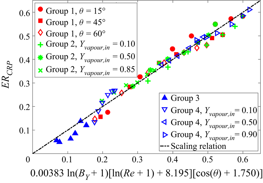
Figure 19. Universal scaling relation of average evaporation rate in CRP.
Table 2. Cases considered for the effect of inflow Reynolds number (Re).
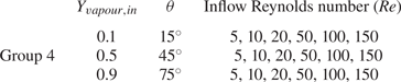
5. Concluding remarks
In this work, a mesoscopic LBM is proposed and applied to simulate the two-component multiphase evaporation in porous media at the pore scale. We consider isothermal systems, and the evaporation in porous media is driven by the difference in vapour concentration from the liquid–gas interface to the far field. Our model is constructed based on the multicomponent multiphase pseudopotential model, with two lattice Boltzmann equations for solving the volatile component (water and its vapour) and the non-condensible component (NCG, dry air), respectively. The lattice Boltzmann cascaded collision operator is employed to improve numerical stability and flexibility. Through Chapman–Enskog multiscale analysis, we show that our model reproduces the Navier–Stokes equations for the two-component mixture in the low-Mach-number limit. An effective binary transport mechanism between vapour and dry air in the gas phase, resulting from the difference between component velocity and mixture velocity, can be automatically captured in our model. Based on the two-component Stefan problem, we show that our model follows Fick's diffusion law and has the flexibility to tune the mass fraction of NCG from 2 % up to 90 %. We propose a scheme to implement the contact angle by extending the well-established single-component geometric function scheme to two-component systems. Based on the steady droplet tests, we show that our proposed scheme can tune the contact angle within a wide range, independently of the component mass fraction. Furthermore, our model is well validated with an evaporation experiment in a microfluidic network.
Our model is applied to study the convective evaporation in a custom-designed dual-porosity medium, characterized by blowing a drier gas mixture over the material surface. Benefiting from its pore-scale feature, the detailed pore-scale dynamics, such as the receding evaporation front and the changing vertical saturation profile, can be directly resolved in our model. We observed a clear transition of the local pore evaporation rate at the material surface, from inflow–high–outflow–low to inflow–low–outflow–high, which is consistent with previous numerical study. Moreover, three main evaporation periods in classical evaporation experiments, i.e. CRP, FRP and RFP, are reproduced in our simulations. A systematic parameter study is carried out to investigate the effect of inflow vapour concentration  ${Y_{vapour,in}}$ and contact angle
  $\theta$ on evaporation dynamics. In the CRP, the average evaporation rate is increased by decreasing
  ${Y_{vapour,in}}$ and scales with the concentration-related mass transfer number
  ${B_Y}$ by
  $E{R_{CRP}} \propto \ln (1 + {B_Y})$. In the RFP, the scaling relation is less prominent since the vapour concentration profiles inside the porous medium are not sensitive to
  ${Y_{vapour,in}}$. The effect of the contact angle
  $\theta$ is twofold: in the CRP, the average evaporation rate increases with decreasing
  $\theta$ by
  $E{R_{CRP}} \propto \cos (\theta )$ since the capillary pumping effect is dominant; in the RFP, the average evaporation rate drops with decreasing
  $\theta$ by
  $\ln (E{R_{RFP}}) \propto - \cos (\theta )$ when the Kelvin effect is significant. Moreover, a universal scaling dependence of average evaporation in the CRP on the inflow vapour concentration
  ${Y_{vapour,in}}$, contact angle
  $\theta$ and inflow Reynolds number Re is found, i.e.
  $E{R_{CRP}} = {k_3}\ln ( {1 + {B_Y}} ) {\cdot } [ {\ln ( {1 + {Re} } ) + {k_2}} ] {\cdot } [ {\cos (\theta ) + {k_1}} ]$, over a comparatively wide range of parameter values,
  ${Y_{vapour,in}} \in [0.1,{{}}0.98]$,
  $\theta \in [{15^ \circ },{{}}{105^ \circ }]$ and
  ${Re} \in [5,150]$.
Supplementary movies
Supplementary movies are available at https://doi.org/10.1017/jfm.2022.1048.
Funding
This work was supported by the Swiss National Science Foundation (Project No. 175793) and the Swiss National Super Computing Center (Project No. s1081 and No. go09).
Declaration of interests
The authors report no conflict of interest.
Appendix A. Chapman–Enskog analysis
Taylor series expansion of (2.1) at  $({\boldsymbol {x}},t)$ yields
 \begin{align} &\Delta t({\partial _t} + {{\boldsymbol{e}}_i} \boldsymbol{\cdot}\boldsymbol{\nabla} )f_i^k + \frac{{\Delta {t^2}}}{2}{({\partial _t} + {{\boldsymbol{e}}_i} \boldsymbol{\cdot}\boldsymbol{\nabla} )^2}f_i^k + O(\Delta {t^3}) \nonumber\\ &\quad ={-} ({{\boldsymbol{\mathsf{M}}}^{ - 1}}{\boldsymbol{\mathsf{N}}^{ - 1}}{\boldsymbol{\mathsf{SN}}}{\boldsymbol{\mathsf{M}}})\left( {f_i^k - f_i^{k,eq}} \right) + \Delta tR_i^k + \frac{{\Delta {t^2}}}{2}({\partial _t} + {{\boldsymbol{e}}_i} \boldsymbol{\cdot} \boldsymbol{\nabla} )R_i^k. \end{align}
Multiplying (A1) by  $\boldsymbol{\mathsf{M}}$ leads to
 \begin{align} ({\boldsymbol{\mathsf{I}}}{\partial _t} + {\boldsymbol{\mathsf{D}}}){{\boldsymbol{m}}^k} + \frac{{\Delta t}}{2}{({\boldsymbol{\mathsf{I}}}{\partial _t} + {\boldsymbol{\mathsf{D}}})^2}{{\boldsymbol{m}}^k} ={-} \frac{{{\boldsymbol{\mathsf{N}}^{ - 1}}{\boldsymbol{\mathsf{SN}}}}}{{\Delta t}}({{\boldsymbol{m}}^k} - {{\boldsymbol{m}}^{k,eq}}) + {{\boldsymbol{C}}^k} + \frac{{\Delta t}}{2}({\boldsymbol{\mathsf{I}}}{\partial _t} + {\boldsymbol{\mathsf{D}}}){{\boldsymbol{C}}^k}, \end{align}
where  ${{\boldsymbol {m}}^k} = {\boldsymbol{\mathsf{M}}}|\,{f_i^k} \rangle$,
  ${{\boldsymbol {m}}^{k,eq}} = {\boldsymbol{\mathsf{M}}}|\,{f_i^{k,eq}} \rangle$,
  ${{\boldsymbol {C}}^k} = {\boldsymbol{\mathsf{M}}}| {R_i^k} \rangle$ and
  ${\boldsymbol{\mathsf{D}}} = {\boldsymbol{\mathsf{M}}}[ {({{\boldsymbol {e}}_i} \boldsymbol {\cdot } \boldsymbol {\nabla } ){\boldsymbol{\mathsf{I}}}} ]{{\boldsymbol{\mathsf{M}}}^{ - 1}}$.
To perform the Chapman–Enskog analysis, the following multiscale expansions are introduced:
 \begin{equation} \left.\begin{gathered} f_i^k = f_i^{k,(0)} + \varepsilon f_i^{k,(1)} + \varepsilon f_i^{k,(2)} + \cdots, \\ {\partial _t} = \varepsilon {\partial _{t_1}} + {\varepsilon ^2}{\partial _{t_2}},\quad {{}} \boldsymbol{\nabla} = \varepsilon \boldsymbol{\nabla},\quad {{\boldsymbol{F}}^k} = \varepsilon {{\boldsymbol{F}}^{k,(1)}},\quad R_i^k = \varepsilon R_i^{k,(1)}. \end{gathered}\right\} \end{equation}
Using these expansions, (A2) can be rewritten in the consecutive order of  $\varepsilon$:
 $$\begin{gather} O({\varepsilon ^0}):{{\boldsymbol{m}}^{k,(0)}} = {{\boldsymbol{m}}^{k,eq}}, \end{gather}$$
 $$\begin{gather}O({\varepsilon ^1}):({\boldsymbol{\mathsf{I}}}{\partial _{t_1}} + {{\boldsymbol{\mathsf{D}}}_1}){{\boldsymbol{m}}^{k,(0)}} ={-} \frac{{{\boldsymbol{\mathsf{N}}^{ - 1}}{\boldsymbol{\mathsf{SN}}}}}{{\Delta t}}{{\boldsymbol{m}}^{k,(1)}} + {{\boldsymbol{C}}^{k,(1)}}, \end{gather}$$
 \begin{gather} O({\varepsilon ^2}):\;{\partial _{t_2}}{{\boldsymbol{m}}^{k,(0)}} + ({\boldsymbol{\mathsf{I}}}{\partial _{t_1}} + {{\boldsymbol{\mathsf{D}}}_1}){{\boldsymbol{m}}^{k,(1)}} + \frac{{\Delta t}}{2}{({\boldsymbol{\mathsf{I}}}{\partial _{t_1}} + {{\boldsymbol{\mathsf{D}}}_1})^2}{{\boldsymbol{m}}^{k,(0)}} \nonumber\\ \quad ={-} \frac{{{\boldsymbol{\mathsf{N}}^{ - 1}}{\boldsymbol{\mathsf{SN}}}}}{{\Delta t}}{{\boldsymbol{m}}^{k,(2)}} + \frac{{\Delta t}}{2}({\boldsymbol{\mathsf{I}}}{\partial _{t_1}} + {{\boldsymbol{\mathsf{D}}}_1}){{\boldsymbol{C}}^{k,(1)}}. \end{gather}
According to (A5), (A6) can be rewritten as
 \begin{equation} O({\varepsilon ^2}):\;{\partial _{t_2}}{{\boldsymbol{m}}^{k,(0)}} + ({\boldsymbol{\mathsf{I}}}{\partial _{t_1}} + {{\boldsymbol{\mathsf{D}}}_1})\left( {{\boldsymbol{\mathsf{I}}} - \frac{{{\boldsymbol{\mathsf{N}}^{ - 1}}{\boldsymbol{\mathsf{SN}}}}}{2}} \right){{\boldsymbol{m}}^{k,(1)}} ={-} \frac{{{\boldsymbol{\mathsf{N}}^{ - 1}}{\boldsymbol{\mathsf{SN}}}}}{{\Delta t}}{{\boldsymbol{m}}^{k,(2)}}. \end{equation}
Here, we need the explicit expressions for  ${\boldsymbol{\mathsf{D}}} = {\boldsymbol{\mathsf{M}}}[ {({{\boldsymbol {e}}_i} \boldsymbol {\cdot } \boldsymbol {\nabla } ){\boldsymbol{\mathsf{I}}}} ]{{\boldsymbol{\mathsf{M}}}^{ - 1}}$ and
  ${\boldsymbol{\mathsf{N}}^{ - 1}}{\boldsymbol{\mathsf{SN}}}$, which can be obtained by the software Matlab. According to (A5), we can obtain the continuity and momentum equations at
  $O(\varepsilon )$ level:
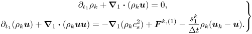 \begin{equation} \left.\begin{gathered} {\partial _{{t_1}}}{\rho _k} + {\boldsymbol{\nabla}_1} \boldsymbol{\cdot} ({\rho _k}{\boldsymbol{u}}) = 0,\\ {\partial _{{t_1}}}({\rho _k}\boldsymbol{u})+ {\boldsymbol{\nabla} _1} \boldsymbol{\cdot} ({\rho _k}{\boldsymbol{uu}}) ={-} {\boldsymbol{\nabla} _1}({\rho _k}c_s^2) + {{\boldsymbol{F}}^{k,(1)}} - \frac{{s_1^k}}{{\Delta t}}{\rho _k}({{\boldsymbol{u}}_k} - {\boldsymbol{u}}). \end{gathered}\right\} \end{equation}
Here, one may notice that the component velocity  ${{\boldsymbol {u}}_k}$ is not necessarily equal to the velocity of the two-component mixture
  ${{\boldsymbol {u}}}$. According to classical diffusion theory (Shan & Doolen Reference Shan and Doolen1996), the velocity difference
  ${{\boldsymbol {u}}_k}-{\boldsymbol {u}}$ is the mass-average diffusion velocity of component k towards the mixture, and therefore
  ${{\boldsymbol {J}}_k} = {\rho _k}({{\boldsymbol {u}}_k} - \boldsymbol {u})$ the mass diffusion flux. Analogously, we have the equations at the
  $O(\varepsilon ^2 )$ level as follows:
 \begin{equation} \left.\begin{gathered} {\partial _{{t_2}}}{\rho _k} + {\boldsymbol{\nabla}_1} \boldsymbol{\cdot} \left[ {\left( {1 - \frac{{{s_1}}}{2}} \right){{\boldsymbol{J}}_k}} \right] = 0,\\ {\partial _{{t_2}}}({\rho _k}{u_x}) + \frac{1}{2}{\partial _{x_1}}\left[ {\left( {1 - \frac{{{s_b}}}{2}} \right)m_3^{k,(1)} + \left( {1 - \frac{{{s_\nu }}}{2}} \right)m_4^{k,(1)}} \right] \\ + \frac{1}{2}{\partial _{y_1}}\left[ {\left( {1 - \frac{{{s_v}}}{2}} \right)m_5^{k,(1)}} \right] + {\partial _{{t_1}}}\left[ {\left( {1 - \frac{{{s_1}}}{2}} \right){J_{k,x}}} \right] = 0,\\ {\partial _{{t_2}}}({\rho _k}{u_y})+ \frac{1}{2}{\partial _{y_1}}\left[ {\left( {1 - \frac{{{s_b}}}{2}} \right)m_3^{k,(1)} - \left( {1 - \frac{{{s_\nu }}}{2}} \right)m_4^{k,(1)}} \right]\\ + \frac{1}{2}{\partial _{x_1}}\left[ {\left( {1 - \frac{{{s_\nu }}}{2}} \right)m_5^{k,(1)}} \right] + {\partial _{{t_1}}}\left[ {\left( {1 - \frac{{{s_1}}}{2}} \right){J_{k,y}}} \right] = 0, \end{gathered}\right\} \end{equation}
where we have assumed  $({{\boldsymbol {u}}^x} - \boldsymbol {u}) \sim O({\varepsilon ^2})$ and the higher-order terms have been neglected (Chai & Zhao Reference Chai and Zhao2012). By using the
  $O(\varepsilon )$ equation once again, we can obtain
 \begin{equation} \left.\begin{gathered} {\partial _{t_1}}m_3^{k,eq} + {\partial _{x_1}}(m_1^{k,eq} + m_7^{k,eq}) + {\partial _{y_1}}(m_2^{k,eq} + m_6^{k,eq}) ={-} \frac{{{s_b}}}{{\Delta t}}m_3^{k,(1)} + C_3^{k,(1)},\\ {\partial _{t_1}}m_4^{k,eq} + {\partial _{x_1}}(m_1^{k,eq} - m_7^{k,eq}) - {\partial _{y_1}}(m_2^{k,eq} - m_6^{k,eq}) ={-} \frac{{{s_2}}}{{\Delta t}}m_4^{k,(1)} + C_4^{k,(1)},\\ {\partial _{t_1}}m_5^{k,eq} + {\partial _{x_1}}m_6^{k,eq} + {\partial _{y_1}}m_7^{k,eq} ={-} \frac{{{s_2}}}{{\Delta t}}m_5^{k,(1)} + C_5^{k,(1)}. \end{gathered}\right\} \end{equation}
Here, the following relations can be obtained according to (A8):
 \begin{equation} {\partial _{t_1}}({\rho _k}{u_a}{u_\beta }) \approx{-} {u_\alpha }{\partial _{\beta _1}}(\rho c_s^2) - {u_\beta }{\partial _{\alpha_1}}(\rho c_s^2) + {u_\alpha }F_\beta ^{k,(1)} + {u_\beta }F_\alpha^{k,(1)}. \end{equation}
Substituting (A11) into (A10), we can obtain
 \begin{equation} \left.\begin{gathered} m_3^{k,(1)} ={-} \frac{{2\Delta t}}{{{s_b}}}{\rho _k}c_s^2({\partial _{x_1}}{u_x} + {\partial _{y_1}}{u_y}),\\ m_4^{k,(1)} ={-} \frac{{2\Delta t}}{{{s_\nu }}}{\rho _k}c_s^2({\partial _{x_1}}{u_x} - {\partial _{y_1}}{u_y}),\\ m_5^{k,(1)} ={-} \frac{{2\Delta t}}{{{s_\nu }}}{\rho _k}c_s^2({\partial _{x_1}}{u_y} + {\partial _{y_1}}{u_x}). \end{gathered}\right\} \end{equation}
Then, (A9) can be rewritten as
 \begin{equation} \left.\begin{gathered} {\partial _{{t_2}}}{\rho _k} + {\boldsymbol{\nabla} _1} \boldsymbol{\cdot} \left[ {\left( {1 - \frac{{{s_1}}}{2}} \right){{\boldsymbol{J}}_k}} \right] = 0,\\ {\partial _{{t_2}}}({\rho _k}{u_x})+{\partial _{{t_1}}}\left[ {\left( {1 - \frac{{{s_1}}}{2}} \right){J_{k,x}}} \right] = {\partial _{x_1}}\left[ {{\rho _k}{\nu _b}\left( {{\boldsymbol{\nabla} _1} \boldsymbol{\cdot} {\boldsymbol{u}}} \right) + {\rho _k}\nu \left( {{\partial _{x_1}}{u_x} - {\partial _{y_1}}{u_y}} \right)} \right]\\ + {\partial _{y_1}}\left[ {{\rho _k}\nu \left( {{\partial _{x_1}}{u_y} + {\partial _{y_1}}{u_x}} \right)} \right],\\ {\partial _{{t_2}}}({\rho _k}{u_y})+ {\partial _{{t_1}}}\left[ {\left( {1 - \frac{{{s_1}}}{2}} \right){J_{k,y}}} \right] = {\partial _{y_1}}\left[ {{\rho _k}{\nu _b}\left( {{\boldsymbol{\nabla} _1} \boldsymbol{\cdot} {\boldsymbol{u}}} \right) + {\rho _k}\nu \left( {{\partial _{y_1}}{u_y} - {\partial _{x_1}}{u_x}} \right)} \right]\\ + {\partial _{x_1}}\left[ {{\rho _k}\nu \left( {{\partial _{x_1}}{u_y} + {\partial _{y_1}}{u_x}} \right)} \right], \end{gathered}\right\} \end{equation}
where  $\nu = c_s^2\Delta t(1/{s_\nu } - 1/2)$ and
  ${\nu _b} = c_s^2\Delta t(1/{s_b} - 1/2)$ are the component kinetic and bulk viscosities, respectively.
Combining (A8) and (A13) through  ${\partial _t} = \varepsilon {\partial _{t1}} + {\varepsilon ^2}{\partial _{t2}}$, we can obtain
 \begin{equation} \left.\begin{gathered} {\partial _t}{\rho _k} + \boldsymbol{\nabla} \boldsymbol{\cdot} ({\rho _k}{\boldsymbol{u}}) + \boldsymbol{\nabla}\boldsymbol{\cdot} \left[ {\left( {1 - \frac{{{s_1}}}{2}} \right){{\boldsymbol{J}}_k}} \right] = 0,\\ {\partial _t}({\rho _k}{\boldsymbol{u}}) + \boldsymbol{\nabla}\boldsymbol{\cdot} ({\rho _k}{\boldsymbol{uu}}) + {\partial _t}\left[ {\left( {1 - \frac{{{s_1}}}{2}} \right){{\boldsymbol{J}}_k}} \right] ={-} {\boldsymbol{\nabla}}({\rho _k}c_s^2) + {{\boldsymbol{F}}^k} \\ + \boldsymbol{\nabla}\boldsymbol{\cdot} \left[ {{\rho _k}{\nu}\left( {{\boldsymbol{\nabla}_1}{\boldsymbol{u}} + {\boldsymbol{\nabla}_1}{{\boldsymbol{u}}^{\top}}} \right) + {\rho _k}({\nu _{b}} - {\nu})(\boldsymbol{\nabla}\boldsymbol{\cdot} {\boldsymbol{u}}){\boldsymbol{\mathsf{I}}}} \right] - s_1{{\boldsymbol{J}}_k}/\Delta t . \end{gathered}\right\} \end{equation}
Due to the zero net mass diffusion flux, we have  $\sum \nolimits _k {{{\boldsymbol {J}}_k}} = 0$, and therefore we can further obtain the Navier–Stokes equations for the mixture:
 \begin{equation} \left.\begin{gathered} {\partial _t}\rho + \boldsymbol{\nabla}\boldsymbol{\cdot} (\rho {\boldsymbol{u}}) = 0,\\ {\partial _t}(\rho {\boldsymbol{u}}) + \boldsymbol{\nabla} \boldsymbol{\cdot} (\rho {\boldsymbol{uu}}) ={-} \boldsymbol{\nabla} (\rho c_s^2) + {\boldsymbol{F}} + \boldsymbol{\nabla} \boldsymbol{\cdot} \left[ {\rho \nu \left( {\boldsymbol{\nabla} {\boldsymbol{u}} + \boldsymbol{\nabla} {{\boldsymbol{u}}^{\top}}} \right) + \rho ({\nu _b} - \nu )(\boldsymbol{\nabla}\boldsymbol{\cdot} {\boldsymbol{u}}){\boldsymbol{\mathsf{I}}}} \right]. \end{gathered}\right\} \end{equation}
According to the continuity equation for the mixture, we can rewrite the component mass equation as
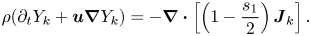 \begin{equation} \rho ({\partial _t}{Y_k} + {\boldsymbol{u}}\boldsymbol{\nabla} {Y_k}) ={-} \boldsymbol{\nabla} \boldsymbol{\cdot} \left[ {\left( {1 - \frac{{{s_1}}}{2}} \right){{\boldsymbol{J}}_k}} \right]. \end{equation}
The component momentum equation at  ${t_1}$ scale can be rewritten as
 \begin{equation} {\rho _k}({\partial _{{t_1}}}{\boldsymbol{u}} + {\boldsymbol{u}}{\boldsymbol{\nabla} _1}{\boldsymbol{u}}) ={-} {\boldsymbol{\nabla}_1}{p_k} + {\boldsymbol{F}}_1^k - \frac{{{s_1}}}{{\Delta t}}{{\boldsymbol{J}}_k}. \end{equation}
The mixture momentum equation at  ${t_1}$ scale can be written as
 \begin{equation} \rho ({\partial _{{t_1}}}{\boldsymbol{u}} + {\boldsymbol{u}}{\boldsymbol{\nabla}_1}{\boldsymbol{u}}) ={-} {\boldsymbol{\nabla}_1}p + {{\boldsymbol{F}}_1}. \end{equation}
Therefore, we have
 \begin{equation} \frac{{{s_1}}}{{\Delta t}}{{\boldsymbol{J}}_k} ={-} {\boldsymbol{\nabla}_1}{p_k} + {Y_k}{\boldsymbol{\nabla}_1}p + (1 - {Y_k}){\boldsymbol{F}}_1^k - {Y_k}{\boldsymbol{F}}_1^{\bar{k}}. \end{equation}
If the system is at mechanical equilibrium, the total pressure gradient is zero (at least for the planar interface system). Far from the liquid–gas interface, the intra-component force goes to zero and the inter-component forces approximately cancel with each other. Under such conditions, (A19) can be further simplified as
 \begin{equation} \left( {1 - \frac{{{s_1}}}{2}} \right){{\boldsymbol{J}}_k} ={-} \left( {\frac{1}{{{s_1}}} - \frac{1}{2}} \right)\Delta t{\boldsymbol{\nabla}_1}{p_k} ={-} \rho {\alpha _0}{\boldsymbol{\nabla}_1}{Y_k}. \end{equation}
If both the components are ideal gases, i.e.  ${p_k} = {\rho _k}c_s^2$, we have
  ${\alpha _0} = (1/{s_1} - 1/2)c_s^2\Delta t$. Substituting (A20) into (A16), the following convection–diffusion equation is obtained:
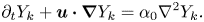 \begin{equation} {\partial _t}{Y_k} + {\boldsymbol{u}} \boldsymbol{\cdot}\boldsymbol{\nabla} {Y_k} = {\alpha _0}{\nabla ^2}{Y_k}. \end{equation}
Appendix B. Three-dimensional simulations
In this appendix, we consider a 3-D simulation of the microfluidic evaporation experiment in § 3.3. In § 2.3, we have extended the geometric-function-based contact angle scheme to two-component multiphase systems. However, the extension to three dimensions is not straightforward due to the fact that in two dimensions there are only two possible characteristic lines making a prescribed contact angle  ${\theta _p}$ with
  ${{\boldsymbol {n}}_s}$ (as shown in figure 1a), but in 3-D space the characteristic lines that make an angle
  ${\theta _p}$ with
  ${{\boldsymbol {n}}_s}$ form a circular cone surface around
  ${{\boldsymbol {n}}_s}$ (Akai, Bijeljic & Blunt Reference Akai, Bijeljic and Blunt2018). Recently, Li et al. (Reference Li, Yu and Luo2019) proposed an improved virtual density scheme to implement the contact angle, which works well in both two and three dimensions, while its extension to two-component systems has not been developed yet. Since our aim is to show that some of the differences between the 2-D simulations and the experiments can be improved when using 3-D simulations, we only consider a single-component system (liquid water and water vapour). The previously proposed 3-D CLBM based on the D3Q19 lattice (Fei et al. Reference Fei, Yang, Chen, Mo and Luo2020) is used in the single-component multiphase flow, and the contact angle scheme by Li et al. (Reference Li, Yu and Luo2019) is employed to implement the contact angle. Following Zhao et al. (Reference Zhao, Qin, Kang, Derome and Carmeliet2022), the evaporation is triggered by setting a low boundary vapour density, i.e.
  ${\rho _{out}} = 0.75\rho _v^s$. The computational domain is resolved by
  $684\Delta x \times 730\Delta x \times 10\Delta x$ lattices, and the other settings are kept the same as in 2-D simulations. The liquid distribution in the network at different liquid saturations S is presented in figure 20. Compared with the 2-D simulation results in figure 7(a), it is seen that the isolated liquid patches almost disappear in 3-D simulations and the simulation results agree better with the experimental results in figure 7(b). Nevertheless, the present 3-D simulation is preliminary and more elaborate 3-D simulations need to be conducted in the future with an appropriate extension of the numerical model.
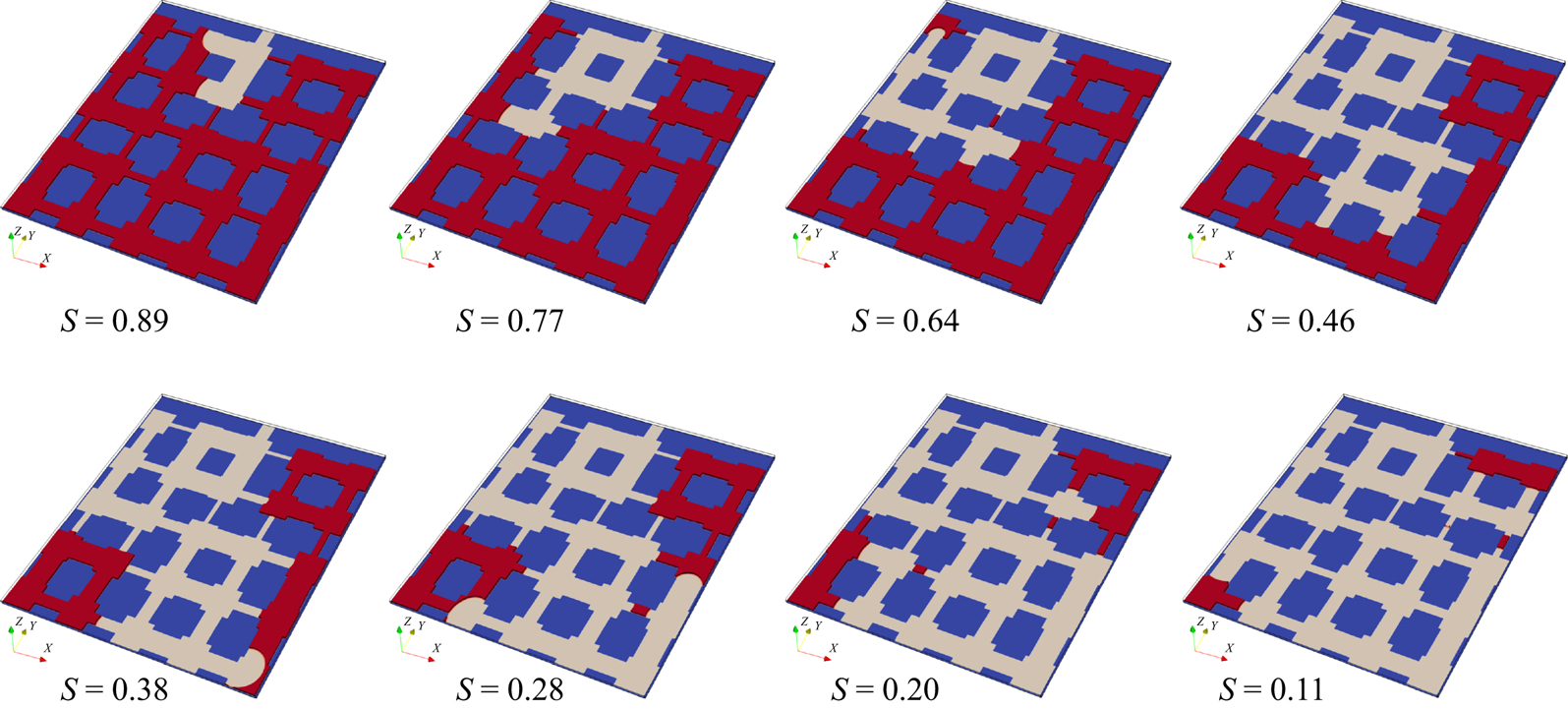
Figure 20. Evolution of the liquid distribution in the network at different liquid saturations S.


 Open access