


1. Introduction
Elastocapillarity involving the interplay of capillary and elastic forces has received much attention in recent years (Style et al. Reference Style, Jagota, Hui and Dufresne2017; Bico, Reyssat & Roman Reference Bico, Reyssat and Roman2018; Andreotti & Snoeijer Reference Andreotti and Snoeijer2020). This is due to the fact that elastocapillary phenomena are common in our everyday life, e.g. the clumping of wet hair or paintbrush bristles, the buckling of pulmonary airways, etc. Elastocapillarity is also relevant to many industrial applications at the microscopic scale. For example, in microelectromechanical systems (MEMS), it is known that elastocapillary interactions are responsible for the collapse of microstructures in humid environments. This leads to an irreversible system failure and poses major fabrication difficulties in MEMS.
There has been much work on elastocapillary problems involving elastic slabs. Consider a liquid drop deposited on an elastic substrate for example. Interesting phenomena occur at the contact line where the fluid interface meets the solid surface. For example, the substrate can be deformed by the capillary force of the drop, resulting in a wetting ridge (Shanahan Reference Shanahan1987b; Carré, Gastel & Shanahan Reference Carré, Gastel and Shanahan1996; Pericet-Cámara et al. Reference Pericet-Cámara, Best, Butt and Bonaccurso2008; Das et al. Reference Das, Marchand, Andreotti and Snoeijer2011; Jerison et al. Reference Jerison, Xu, Wilen and Dufresne2011; Limat Reference Limat2012; Style et al. Reference Style, Boltyanskiy, Che, Wettlaufer, Wilen and Dufresne2013; Hui & Jagota Reference Hui and Jagota2014; Pozrikidis & Hill Reference Pozrikidis and Hill2014; Bardall, Daniels & Shearer Reference Bardall, Daniels and Shearer2018); the contact angle of the fluid interface may violate the classical Young–Dupré equation (Shanahan Reference Shanahan1987b; Style & Dufresne Reference Style and Dufresne2012; Style et al. Reference Style, Boltyanskiy, Che, Wettlaufer, Wilen and Dufresne2013). The deformation of the substrate also affects the contact line dynamics (Shanahan Reference Shanahan1988; Carré et al. Reference Carré, Gastel and Shanahan1996; Extrand & Kumagai Reference Extrand and Kumagai1996; Kajiya et al. Reference Kajiya, Daerr, Narita, Royon, Lequeux and Limat2013; Karpitschka et al. Reference Karpitschka, Das, van Gorcum, Perrin, Andreotti and Snoeijer2015; Howland et al. Reference Howland, Antkowiak, Castrejón-Pita, Howison, Oliver, Style and Castrejón-Pita2016).
When the substrate is thin, its deformation is roughly uniform across the thickness thus it can be effectively modelled by a two-dimensional (2-D) elastic sheet with bending and stretching energies. The bending of such an elastic sheet by capillary forces occurs on the length scale  $l_B = \sqrt {{E t^3}/{24(1-\nu ^2)\gamma }}$, where
  $\gamma$ is the fluid surface tension, and
  $E$,
$E$,  $\nu$ and
  $t$ are the Young's modulus, the Poisson ratio and the thickness of the substrate, respectively (Bico et al. Reference Bico, Reyssat and Roman2018). Bending of elastic sheets leads to an enhancement of capillary rise (Kim & Mahadevan Reference Kim and Mahadevan2006). It also enables elastic sheets to spontaneously wrap liquid droplets, a process called capillary origami in the literature. Py et al. (Reference Py, Reverdy, Doppler, Bico, Roman and Baroud2007, Reference Py, Reverdy, Doppler, Bico, Roman and Baroud2009) derived a folding criterion in terms of the size of the sheet from the balance of elastic and capillary effects. They also showed that folded structures can be controlled by tailoring the initial sheet geometry. Antkowiak et al. (Reference Antkowiak, Audoly, Josserand, Neukirch and Rivetti2011) showed the folding process was accelerated using drop impact, and different three-dimensional (3-D) structures were produced from a given sheet by varying the impact speed and the location of impact. Folding of an elastic sheet around a deposited drop was studied by Neukirch, Antkowiak & Marigo (Reference Neukirch, Antkowiak and Marigo2013) using a variational approach. Brubaker & Lega (Reference Brubaker and Lega2016) derived equilibrium equations for folded origami systems with pinned contact lines by minimizing the sum of the interfacial and elastic energies; the work was later extended to the case of a partial wetting droplet on inextensible elastic sheets in two dimensions (Brubaker Reference Brubaker2019). The folded structure was also investigated based on governing equations obtained from mechanical equilibrium (Péraud & Lauga Reference Péraud and Lauga2014). When the sheet is ultra-thin with negligible bending energy, the final shape of the folded structure is determined by geometric constraints which only involve interfacial energies (Paulsen et al. Reference Paulsen, Démery, Santangelo, Russell, Davidovitch and Menon2015). On an ultra-thin elastic sheet, the capillary force from a deposited drop can induce wrinkles. The size of the wrinkled region, the pattern of wrinkling as well as its mechanism have been studied in many work, e.g. Huang et al. (Reference Huang, Juszkiewicz, de Jeu, Cerda, Emrick, Menon and Russell2007), Vella, Adda-Bedia & Cerda (Reference Vella, Adda-Bedia and Cerda2010), Schroll et al. (Reference Schroll, Adda-Bedia, Cerda, Huang, Menon, Russell, Toga, Vella and Davidovitch2013) and Davidovitch & Vella (Reference Davidovitch and Vella2018).
In contrast to the large body of work on static problems involving thin sheets, there have been very few studies concerning the dynamics. Duprat, Aristoff & Stone (Reference Duprat, Aristoff and Stone2011) studied the dynamics of the rise of a wetting liquid between flexible sheets. Bradley et al. (Reference Bradley, Box, Hewitt and Vella2019); Bradley, Hewitt & Vella (Reference Bradley, Hewitt and Vella2021) and Zhang & Qian (Reference Zhang and Qian2022) investigated the spontaneous movement of a liquid droplet in a thin channel formed by elastic sheets, a process called bendotaxis. Taroni & Vella (Reference Taroni and Vella2012) developed a dynamic model to study the elastocapillary interaction of a liquid drop with the bounding elastic beams and investigated equilibrium configurations of the system as the steady limit of the dynamics. The model took into account the effects of both the Laplace pressure in the bulk of the droplet and the line force at the contact line on the deflection of the beams. All these works were based on the lubrication approximation for the fluid dynamics. Antkowiak et al. (Reference Antkowiak, Audoly, Josserand, Neukirch and Rivetti2011) developed a 2-D model for the folding dynamics of elastic sheets induced by drop impact. There, after the initial spreading of the drop, the fluid dynamics was assumed to relax sufficiently fast so that the drop was in quasi-static state with the contact lines pinned and separated by a prescribed distance. Only the dynamics of the elastic sheets was considered in their model. Nevertheless, good agreements of the dynamics and the final shape of the sheet with experiments were obtained.
Aside from the above theoretical work, effective numerical methods were also proposed to simulate the dynamics. For example, Alben et al. (Reference Alben, Gorodetsky, Kim and Deegan2019) developed semi-implicit numerical methods to approximate the over-damped dynamics of elastic sheets. The numerical methods have a better stability property as compared to explicit discretization methods, thus allow larger time steps. Barrett, Garcke & Nürnberg (Reference Barrett, Garcke and Nürnberg2017, Reference Barrett, Garcke and Nürnberg2020) developed parametric finite element methods to simulate surface evolutions, e.g. the dynamics of biomembranes with the Willmore energy (Helfrich Reference Helfrich1973). Numerical methods were also developed for systems involving moving contact lines, e.g. Wouters et al. (Reference Wouters, Aouane, Krüger and Harting2019), Pepona et al. (Reference Pepona, Shek, Semprebon, Krüger and Kusumaatmaja2021) and Chen & Zhang (Reference Chen and Zhang2022). These methods use the lattice Bolztmann method or dissipative particle dynamics to model the fluid dynamics and various discrete models for the elastic sheet. The coupling of the fluids and the sheet is usually achieved through interactions between the fluid and solid particles.
In the current work, we focus on the dynamics of elastocapillarity. Specifically, we derive a thermodynamically consistent model for the dynamics of two immiscible fluids or two phases of one fluid on a thin and inextensible elastic sheet in two dimensions. The fluid dynamics is modelled by the Stokes equations. The elastic sheet is characterized by the Willmore bending energy and a local inextensibility constraint. This type of elastic sheet is widely used in modelling vesicles (Kusumaatmaja et al. Reference Kusumaatmaja, Li, Dimova and Lipowsky2009; Kusumaatmaja & Lipowsky Reference Kusumaatmaja and Lipowsky2011; Zhao, Spann & Shaqfeh Reference Zhao, Spann and Shaqfeh2011; Yazdani & Bagchi Reference Yazdani and Bagchi2012; Zhao & Shaqfeh Reference Zhao and Shaqfeh2013; Farutin & Misbah Reference Farutin and Misbah2014; Luo & Bai Reference Luo and Bai2015). The total energy of the system consists of the interfacial and bending energies. We follow principles of non-equilibrium thermodynamics to derive the simplest interfacial and boundary conditions. We obtain these conditions from the consideration of the energy dissipation of the dynamical system. Specifically, we identify the relevant fluxes and their corresponding forces in the energy dissipation, then we connect these fluxes and their corresponding forces using constitutive relations, e.g. linear functions as the simplest one. This energy-based framework is rather general and standard. It has been used in earlier works, for example, to derive boundary conditions at the moving contact line on rigid solid substrates (Ren, Hu & Weinan Reference Ren, Hu and Weinan2010; Ren & Weinan Reference Ren and Weinan2011) and for the moving contact line problem involving soluble surfactants (Zhao, Ren & Zhang Reference Zhao, Ren and Zhang2021). For the current problem, the derived model consists of the Stokes equations for the fluid dynamics, the standard conditions on the fluid interface, the kinematic and inextensibility conditions of the sheet as well as the boundary conditions on the sheet and at the moving contact line. These boundary conditions can be phrased as the balance of various forces.
(i) In the tangential direction of the sheet, the fluid shear stress, the friction force and the gradient of the sheet tension balance each other (see (3.17a) and (3.18)). In the normal direction of the sheet, the fluid normal stress is balanced by the forces arising from the surface and bending energies (see (3.17b)).
(ii) At the moving contact line, the Young stress arising from the deviation of the contact angle from the equilibrium Young's angle, the friction force and the jump of the sheet tension balance each other in the sheet's tangential direction (see (3.22b) and (3.23)). The tension of the fluid interface balances the jump of the curvature gradient of the sheet in the normal direction (see (3.22a)).
In this model, the energy of the system is dissipated through three channels: the viscous force in the bulk of the fluids, the friction at the fluid–sheet interface and the friction at the moving contact line.
Using this model, we simulate the relaxation dynamics of a droplet on an elastic sheet and the droplet transport driven by bendotaxis. Bendotaxis is a mechanism for droplet self-transport in a thin channel formed by two deformable sheets. The sheets are fixed at one end of the channel and free to move at the other end. A droplet confined in the channel moves simultaneously towards the free end as a result of the interaction of the elastic and capillary forces. Understanding the transport dynamics is important for industrial applications, e.g. in designing self-cleaning surfaces. In this work, we employ the derived model to investigate the mechanism of bendotaxis as well as the effects of the droplet wettability and the sheet stiffness on the dynamics. The numerical method in both applications is a finite element method based on a weak formulation of the model. The method is an extension of the parametric finite element method (Barrett et al. Reference Barrett, Garcke and Nürnberg2020) to problems involving moving contact lines.
The rest of the paper is organized as follows. In § 2, we consider the static problem. We first introduce the energy then review the governing equations for the equilibrium system. In § 3, we consider the dynamical problem. We derive the boundary conditions on the elastic sheet and at the moving contact line from the consideration of thermodynamics. Sections 4 and 5 are devoted to applications. We use the derived model to simulate the relaxation dynamics of a droplet on an elastic sheet in § 4 and the droplet motion driven by bendotaxis in § 5. The paper is concluded in § 6.
2. Energetics
We consider the system of two immiscible fluids (fluid 1 and fluid 2) in contact with an elastic sheet in the two-dimensional space, as shown in figure 1. The two fluid regions are denoted by  $\varOmega _1$ and
  $\varOmega _2$, respectively. The sheets in contact with fluid 1 and fluid 2 are denoted by
  $\varSigma _1$ and
  $\varSigma _2$, respectively. The whole sheet
  $\varSigma _1\cup \varSigma _2$ is denoted by
  $\varXi$. The contact lines are denoted by
  $\varLambda$. Furthermore, we denote the unit tangent vector to
  $\varSigma _i\ (i = 1,2)$ by
  $\boldsymbol {\tau }$. The unit normal vector to
  $\varSigma _i\ (i = 1,2,3)$ is denoted by
  ${\boldsymbol n}$, where
  ${\boldsymbol n}$ points away from the fluid region on the sheet and from
  $\varOmega _1$ to
  $\varOmega _2$ on the fluid–fluid interface. The curvature
  $\kappa$ of
  $\varSigma _i$ is defined as
 \begin{equation} \kappa =
\left\{\begin{array}{@{}ll} \boldsymbol{\nabla}_s
\boldsymbol{\cdot} {\boldsymbol n}, & \text{on }
\varSigma_1, \varSigma_2, \\ -\boldsymbol{\nabla}_s
\boldsymbol{\cdot} {\boldsymbol n}, & \text{on }
\varSigma_3, \end{array}\right.
\end{equation}
\begin{equation} \kappa =
\left\{\begin{array}{@{}ll} \boldsymbol{\nabla}_s
\boldsymbol{\cdot} {\boldsymbol n}, & \text{on }
\varSigma_1, \varSigma_2, \\ -\boldsymbol{\nabla}_s
\boldsymbol{\cdot} {\boldsymbol n}, & \text{on }
\varSigma_3, \end{array}\right.
\end{equation}
where  $\boldsymbol {\nabla }_s$ is the surface gradient operator and the negative sign is due to the fact that
  ${\boldsymbol n}$ points upwards on
  $\varSigma _3$. Furthermore, let
  $\boldsymbol {m}_i$ be the unit conormal vector of
  $\varSigma _i\ (i=1,2,3)$ at the contact line, as shown in figure 1(b).

Figure 1. (a) A droplet on an elastic sheet confined in a box. (b) The three interfaces near the contact line.
The total free energy of the system is given by
 \begin{equation} \mathcal{E} = \sum_{i=1}^3 \gamma_i |\varSigma_i| + \frac{c_b}2 \int_{\varXi}\kappa^2\,\mathrm{d}s, \end{equation}
where the first term models the interfacial energy and the second term, known as the Willmore energy, models the bending energy of the sheet. Here,  $\gamma_i\ (i=1, 2, 3)$ are the interfacial tension coefficients of the fluid–sheet and fluid–fluid interfaces,
  $|\varGamma_i|\ (i=1, 2, 3)$ are the arc lengths of the interfaces and
  $c_b$ is the bending modulus of the sheet.
The static profiles of the fluid–fluid interface and the sheet as well as the contact angle can be obtained by minimizing the above energy under the area conservation constraint. In a related work (Zhang, Yao & Ren Reference Zhang, Yao and Ren2020), we studied the equilibrium configuration of a droplet on an elastic membrane in two and three dimensions. The 2-D membrane model took the same form as the one considered here in (2.2). In the following, we briefly review the main results regarding the equilibrium equations in 2-D as well as their asymptotic solutions in the limits of large and small bending modulus, respectively. We note that such a variational approach has been used in earlier work and similar equilibrium equations have been derived (Shanahan Reference Shanahan1987a; Neukirch et al. Reference Neukirch, Antkowiak and Marigo2013; Brubaker Reference Brubaker2019). For example, under the assumption of radial symmetry, equilibrium equations were derived by variation of the total energy, where the sheet elastic energy was described by the bending energy (Shanahan Reference Shanahan1985, Reference Shanahan1987a) and the FvK model consisting of both stretching and bending energies (Olives Reference Olives1993, Reference Olives1996), respectively. More recently, a variational approach was employed to study equilibrium configurations of capillary folding in two dimensions (Neukirch et al. Reference Neukirch, Antkowiak and Marigo2013; Brubaker Reference Brubaker2019) and in three dimensions using the FvK model with pinned contact line (Brubaker & Lega Reference Brubaker and Lega2016).
The governing equations for the static configuration of the system read
 \begin{gather} \gamma_i\kappa -c_b\left(\Delta_s\kappa +\frac12\kappa^3\right)-\lambda_i=0,\quad\text{on }\varSigma_i\ (i=1,2), \end{gather}
 \begin{gather}-\gamma_3 \kappa +\lambda_2-\lambda_1=0,\quad\text{on }\varSigma_3, \end{gather}
 \begin{gather}{[}\![\kappa]\!]^1_2=0,\quad \gamma_3\boldsymbol{m}_3-(\gamma_2-\gamma_1)\boldsymbol{m}_1+c_b \left(\boldsymbol{m}_1\boldsymbol{\cdot}[\![\boldsymbol{\nabla}_s\kappa ]\!]^1_2\right){\boldsymbol n} |_\varXi=\boldsymbol{0}, \quad\text{at }\varLambda, \end{gather}
 \begin{gather}\kappa=0, \quad \gamma_2\cos\theta_w+c_b\left(\boldsymbol{m}_w\boldsymbol{\cdot}\boldsymbol{\nabla}_s\kappa\right)\sin\theta_w=0,\quad\text{at }\partial\varXi, \end{gather}
where  $\lambda _1$ and
  $\lambda _2$ are Lagrange multipliers for the conservation of the area of
  $\varOmega _1$ and
  $\varOmega _2$, respectively, and
  ${\boldsymbol n}|_{\varXi }$ is the unit normal vector of the sheet at the contact line. The last equation is the natural boundary condition at the boundary of the sheet, where
  $\theta _w\in [0,{\rm \pi} ]$ is the angle between the downward tangent vector of the wall
  $\varSigma _4$ and the unit conormal vector
  $\boldsymbol {m}_w$ of the sheet, as depicted in figure 1(a). From the contact line condition (2.3c), we see that the Young–Dupré equation
  $\gamma _3\cos \theta _Y=\gamma _2-\gamma _1$ holds in the tangent direction of the sheet with
  $\theta _Y=\cos ^{-1}(\boldsymbol {m}_3\boldsymbol {\cdot }\boldsymbol {m}_1)$ being the Young's angle. In addition, we have
  $\gamma _3\sin \theta _Y=-c_b (\boldsymbol {m}_1\boldsymbol {\cdot }[\![\boldsymbol {\nabla }_s \kappa ]\!]^1_2)$ in the normal direction of the sheet, which states that the surface tension force in the normal direction is balanced by the force resulting from the jump of
  $\boldsymbol {\nabla }_s \kappa$ across the contact line. We note that a sheet with the inextensibility constraint (see (3.6)) satisfies the same equilibrium equations in (2.3), where the constant Lagrange multiplier for the constraint is absorbed into the surface tension.
Asymptotic solutions were obtained for the above system in the limits as  $c_b$ tends to
  $+\infty$ and
  $0^+$, respectively (Zhang et al. Reference Zhang, Yao and Ren2020). In the stiff limit as
  $c_b\rightarrow +\infty$, the leading order solution is given by the configuration in which a circular droplet sits on a rigid substrate with the Young's contact angle. In the soft limit as
  $c_b\rightarrow 0^+$, the sheet profile exhibits a transition layer in the vicinity of the contact line, and leading-order solutions in the inner (transition) and outer regions were obtained using the matched asymptotic technique. While the real contact angle of the fluid interface still satisfies the Young–Dupré equation, the apparent contact angles obey Neumann's law,
 \begin{equation} \frac{\sin\theta_{12}}{\gamma_3} = \frac{\sin\theta_{23}}{\gamma_1} = \frac{\sin\theta_{31}}{\gamma_2}, \end{equation}
where  $\theta _{ij}$ is the apparent contact angle between the interfaces
  $\varSigma _i$ and
  $\varSigma _j$ in the outer region.
3. Dynamical theory
Next we turn our attention to the dynamical problem. We parametrize the fluid–fluid interface as  ${\boldsymbol {r}}(\zeta, t)$ and the sheet as
  ${\boldsymbol {q}}(\xi, t)$, where
  $\zeta =0$ and
  $\xi =\xi _{{cl}}(t)$ correspond to the (left) contact line
 \begin{equation} {\boldsymbol{r}}(\zeta, t)|_{\zeta=0}={\boldsymbol{q}}(\xi,t)|_{\xi=\xi_{{cl}}(t)}. \end{equation}
The velocity of the fluid interface and the sheet are given by  $\dot {\boldsymbol {r}} = ({\partial }/{\partial t}){\boldsymbol {r}}(\zeta,t)$ and
  $\dot {\boldsymbol {q}} = ({\partial }/{\partial t}){\boldsymbol {q}}(\xi,t)$, respectively. Differentiation of (3.1) with respect to time gives the following kinematic relation at the contact line
 \begin{equation} \dot{\boldsymbol{r}} = \dot{\boldsymbol{q}} + |\partial_{\xi}{\boldsymbol{q}}|\dot{\xi}_{{cl}}\boldsymbol{\tau}, \end{equation}
where  $|\partial _{\xi }{\boldsymbol {q}}|$ is the magnitude of the vector
  $({\partial }/{\partial \xi }){\boldsymbol {q}}(\xi,t)$ and
  $\dot {\xi }_{{cl}}=({\mathrm {d}}/{\mathrm {d}t})\xi _{{cl}}(t)$ is the velocity of the contact line in the reference domain. We assume that the following continuity conditions hold at the contact line
 \begin{equation} [\![{\boldsymbol{q}}]\!]^1_2 = \boldsymbol{0}, \quad [\![\partial_\xi{\boldsymbol{q}}]\!]^1_2 = \boldsymbol{0}, \end{equation}
where  $[\![{\cdot }]\!]^1_2$ denotes the jump across the contact line from
  $\varSigma _2$ to
  $\varSigma _1$. These conditions imply that
  $\boldsymbol {m}_2=-\boldsymbol {m}_1$ at the contact line. The same equations hold at the right contact line depicted in figure 1(a).
We assume that the two fluids are simple incompressible fluids, and their dynamics are governed by the time-independent Stokes equations
 \begin{gather} - \boldsymbol{\nabla} p + \boldsymbol{\nabla}\boldsymbol{\cdot} \boldsymbol{\sigma}_i=\boldsymbol{0}, \end{gather}
 \begin{gather}\boldsymbol{\nabla}\boldsymbol{\cdot}\boldsymbol{u}=0, \end{gather}
in  $\varOmega _i\ (i=1,2)$. Here,
  $\boldsymbol {u}$ is the fluid velocity,
  $p$ is the pressure,
  $\boldsymbol {\sigma }_i =\eta _i(\boldsymbol {\nabla } \boldsymbol {u}+(\boldsymbol {\nabla }\boldsymbol {u})^{\rm T})$ is the viscous stress, and
  $\eta _i$ is the viscosity of fluid
  $i$.
$i$.
As usual, we assume that the fluid velocity is continuous across the fluid–fluid interface and this interface is advected by the fluid velocity
 \begin{gather} [\![\boldsymbol{u}]\!]^1_2 = \boldsymbol{0}, \quad \text{on } \varSigma_3, \end{gather}
 \begin{gather}\dot{\boldsymbol{r}} = \boldsymbol{u}, \quad \text{on } \varSigma_3, \end{gather}
where, with a slight abuse of notation, we use  $[\![{\cdot }]\!]^1_2$ to denote the jump across the fluid–fluid interface from fluid 2 to fluid 1 as well.
The sheet is assumed to be locally inextensible and satisfies the inextensibility condition
 \begin{equation} \boldsymbol{\nabla}_s\boldsymbol{\cdot}\dot{\boldsymbol{q}} = 0. \end{equation}
Furthermore, the sheet obeys the kinematic condition
 \begin{equation} \dot{\boldsymbol{q}}\boldsymbol{\cdot}{\boldsymbol n} = \boldsymbol{u}\boldsymbol{\cdot}{\boldsymbol n}, \quad \text{on } \varXi, \end{equation}
which is also the non-penetration condition for the fluids.
To close the system, we need additional conditions on the fluid–fluid interface and the sheet and at the moving contact line. Conditions at the outer (left, right and top) boundaries are specific to the problem setup and will be discussed later in the applications. The stress conditions on the fluid–fluid interface are well known, and our main interest here is to derive boundary conditions on the sheet and at the moving contact line. However, it will be more convenient for us to treat the conditions on the fluid–fluid interface and those on the elastic sheet on the same footing.
3.1. Thermodynamics and boundary/interface conditions
We will follow the principles of non-equilibrium thermodynamics to look for the simplest interface and boundary conditions. These conditions are consistent with the second law of thermodynamics, which, in the present context, means that the energy dissipation rate of the system has to be non-positive.
The total energy is given in (2.2). Let us compute the time derivative of each term. Since our main focus here is the boundary conditions on the sheet and at the contact line, we will neglect any possible contribution to the energy dissipation from the outer boundaries.
First of all, for the interfacial energy on  $\varSigma _1(t)$, we have
 \begin{align} \frac{\mathrm{d}}{\mathrm{d}t}\int_{\varSigma_1} \gamma_1\,\mathrm{d}s &= \int_{\varSigma_1}\gamma_1(\boldsymbol{\nabla}_s\boldsymbol{\cdot}\dot{\boldsymbol{q}}) \,\mathrm{d}s + \gamma_1\left(|\partial_{\xi}{\boldsymbol{q}}|\dot{\xi}_{{cl}}(\boldsymbol{\tau}\boldsymbol{\cdot}\boldsymbol{m}_1)\right) \Big|_{\varLambda},\nonumber\\ &= \int_{\varSigma_1}\gamma_1\kappa\dot{\boldsymbol{q}}\boldsymbol{\cdot}{\boldsymbol n} \,\mathrm{d}s + \gamma_1\left(|\partial_{\xi}{\boldsymbol{q}}|\dot{\xi}_{{cl}}(\boldsymbol{\tau}\boldsymbol{\cdot}\boldsymbol{m}_1)+\dot{\boldsymbol{q}}\boldsymbol{\cdot}\boldsymbol{m}_1\right)\Big|_{\varLambda}\nonumber\\ &=\int_{\varSigma_1}\gamma_1\kappa\dot{\boldsymbol{q}}\boldsymbol{\cdot}{\boldsymbol n} \,\mathrm{d}s + \gamma_1(\boldsymbol{u}\boldsymbol{\cdot}\boldsymbol{m}_1)\Big|_{\varLambda}, \end{align}
where  $({\cdot })|_{\varLambda }$ denotes the value at the contact line; in the case of multiple contact lines as in figure 1, it is the sum of the values at all the contact lines. In the last step of the above equation, we have used (3.2) and (3.5b). Similarly, for the interfacial energy on
  $\varSigma _2(t)$, we have
 \begin{equation} \frac{\mathrm{d}}{\mathrm{d}t} \int_{\varSigma_2} \gamma_2\,\mathrm{d}s=\int_{\varSigma_2}\gamma_2\kappa\dot{\boldsymbol{q}}\boldsymbol{\cdot}{\boldsymbol n} \,\mathrm{d}s - \gamma_2(\boldsymbol{u}\boldsymbol{\cdot}\boldsymbol{m}_1)\Big|_{\varLambda}, \end{equation}
where we have used the fact that  $\boldsymbol {m}_2=-\boldsymbol {m}_1$ at the contact line. For the interfacial energy on
  $\varSigma _3(t)$, we have
 \begin{equation} \frac{\mathrm{d}}{\mathrm{d}t} \int_{\varSigma_3} \gamma_3 \,\mathrm{d}s ={-}\int_{\varSigma_3}\gamma_3\kappa\boldsymbol{u}\boldsymbol{\cdot}{\boldsymbol n}\,\mathrm{d}s + (\gamma_3\boldsymbol{u}\boldsymbol{\cdot}\boldsymbol{m}_3)\Big|_{\varLambda}, \end{equation}
where we have used (3.5b).
For the Willmore energy of the sheet, we have
 \begin{align} &\frac{\mathrm{d}}{\mathrm{d}t}\int_{\varXi} \frac{c_b}{2}\kappa^2 \,\mathrm{d}s = c_b\sum_{i=1}^2 \int_{\varSigma_i} (-\dot{\boldsymbol{q}}\boldsymbol{\cdot}{\boldsymbol n})\left(\Delta_s\kappa+\frac{1}{2}\kappa^3\right) \,\mathrm{d}s\nonumber\\ &\quad +c_b\left(-[\![\kappa]\!]^1_2\boldsymbol{m}_1\boldsymbol{\cdot}\boldsymbol{\nabla}_s(\dot{\boldsymbol{q}}\boldsymbol{\cdot}{\boldsymbol n}|_{\varXi}) + (\boldsymbol{m}_1\boldsymbol{\cdot}[\![\boldsymbol{\nabla}_s\kappa]\!]^1_2)(\dot{\boldsymbol{q}}\boldsymbol{\cdot}{\boldsymbol n}|_{\varXi}) +\frac{1}{2}[\![\kappa^2]\!]^1_2\boldsymbol{u}\boldsymbol{\cdot}\boldsymbol{m}_1\right)\Big|_{\varLambda}, \end{align}
where  $\Delta _s$ is the Laplace–Beltrami operator. Details for the derivation of this result are provided in Appendix A.
Using the Stokes equation (3.4), we have
 \begin{align} 0&= \sum_{i=1}^2 \int_{\varOmega_i} \boldsymbol{u}\boldsymbol{\cdot}(\boldsymbol{\nabla}\boldsymbol{\cdot}\boldsymbol{\mathsf{T}}_i)\,\mathrm{d}\boldsymbol{x} ={-}\sum_{i=1}^2 \int_{\varOmega_i} \boldsymbol{\nabla}\boldsymbol{u}:\boldsymbol{\mathsf{T}}_i \,\mathrm{d}\boldsymbol{x} + \sum_{i=1}^2 \int_{\partial\varOmega_i}{\boldsymbol n}\boldsymbol{\cdot}\boldsymbol{\mathsf{T}}_i\boldsymbol{\cdot}\boldsymbol{u} \,\mathrm{d}s\nonumber\\ &={-}\sum_{i=1}^2 \int_{\varOmega_i}\frac{1}{2\eta_i}\|\boldsymbol{\sigma}_i\|^2_F \,\mathrm{d}\boldsymbol{x} +\sum_{i=1}^2 \int_{\varSigma_i}{\boldsymbol n}\boldsymbol{\cdot}\boldsymbol{\mathsf{T}}_i\boldsymbol{\cdot}\boldsymbol{u} \,\mathrm{d}s + \int_{\varSigma_3}{\boldsymbol n}\boldsymbol{\cdot}[\![\boldsymbol{\mathsf{T}}]\!]^1_2\boldsymbol{\cdot}\boldsymbol{u} \,\mathrm{d}s, \end{align}
where  $\|\boldsymbol {\cdot }\|_F$ denotes the Frobenius norm,
  $\boldsymbol{\mathsf{T}}_i =-p\boldsymbol {I} + \boldsymbol {\sigma }_i$, and
  $[\![\boldsymbol{\mathsf{T}}]\!]^1_2 = \boldsymbol{\mathsf{T}}_1-\boldsymbol{\mathsf{T}}_2$.
Corresponding to the local inextensibility condition (3.6), we introduce a Lagrange multiplier  $\nu$, named as the tension of the sheet or the sheet tension. Then we have
 \begin{equation} 0 ={-}\sum_{i=1}^2\int_{\varSigma_i} \nu \boldsymbol{\nabla}_s\boldsymbol{\cdot}\dot{\boldsymbol{q}}\,\mathrm{d}s =\sum_{i=1}^2 \int_{\varSigma_i} \left[\boldsymbol{\nabla}_s\nu \boldsymbol{\cdot}\dot{\boldsymbol{q}}-\nu \kappa\dot{\boldsymbol{q}}\boldsymbol{\cdot}{\boldsymbol n} \right]\,\mathrm{d}s - ([\![\nu]\!]^1_2\dot{\boldsymbol{q}}\boldsymbol{\cdot}\boldsymbol{m}_1)\Big|_{\varLambda}. \end{equation}
Combining (3.8), (3.9), (3.10) and (3.11), and using the identities in (3.12) and (3.13), we obtain
 \begin{align}
\frac{\mathrm{d}}{\mathrm{d}t}\mathcal{E}(t)
&={-}\sum_{i=1}^2
\int_{\varOmega_i}\frac{1}{2\eta_i}\|\boldsymbol{\sigma}_i\|^2_F
\,\mathrm{d}\boldsymbol{x}
+\int_{\varSigma_3}\left([\![\boldsymbol{\mathsf{T}}]\!]^1_2\boldsymbol{\cdot}{\boldsymbol
n} -\gamma_3\kappa{\boldsymbol
n}\right)\boldsymbol{\cdot}\boldsymbol{u}
\,\mathrm{d}s\nonumber\\ &\quad +\sum_{i=1}^2
\int_{\varSigma_i} \left({\boldsymbol
n}\boldsymbol{\cdot}\boldsymbol{\mathsf{T}}_i
+\boldsymbol{\nabla}_s\nu +\left[-
c_b(\Delta_s\kappa+\frac{1}{2}\kappa^3)+(\gamma_i-\nu)\kappa\right]{\boldsymbol
n}\right)\boldsymbol{\cdot}\dot{\boldsymbol{q}}
\,\mathrm{d}s\nonumber\\ &\quad +\sum_{i=1}^2
\int_{\varSigma_i} ({\boldsymbol
n}\boldsymbol{\cdot}\boldsymbol{\mathsf{T}}_i\boldsymbol{\cdot}\boldsymbol{\tau})(\boldsymbol{u}-\dot{\boldsymbol{q}})\boldsymbol{\cdot}\boldsymbol{\tau}
\,\mathrm{d}s \nonumber\\ &\quad
-c_b\left([\![\kappa]\!]^1_2\boldsymbol{m}_1\boldsymbol{\cdot}\boldsymbol{\nabla}_s(\dot{\boldsymbol{q}}\boldsymbol{\cdot}{\boldsymbol
n}|_{\varXi}) \right)\Big|_{\varLambda}\nonumber\\ &\quad
+\left(\left([\![\gamma-
\nu+\frac{c_b}{2}\kappa^2]\!]_2^1\boldsymbol{m}_1
+\gamma_3\boldsymbol{m}_3 +
c_b\boldsymbol{m}_1\boldsymbol{\cdot}[\![\boldsymbol{\nabla}_s\kappa]\!]^1_2{\boldsymbol
n}|_{\varXi}\right) \boldsymbol{\cdot}\dot{\boldsymbol{q}}
\right)\Big|_{\varLambda}\nonumber\\ &\quad
+\left(\left([\![\gamma +\frac{c_b}{2}\kappa^2]\!]_2^1
+\gamma_3\boldsymbol{m}_3 \boldsymbol{\cdot}
\boldsymbol{m}_1\right)
\left(\boldsymbol{u}-\dot{\boldsymbol{q}}\right)\boldsymbol{\cdot}\boldsymbol{m}_1\right)\Big|_{\varLambda},
\end{align}
\begin{align}
\frac{\mathrm{d}}{\mathrm{d}t}\mathcal{E}(t)
&={-}\sum_{i=1}^2
\int_{\varOmega_i}\frac{1}{2\eta_i}\|\boldsymbol{\sigma}_i\|^2_F
\,\mathrm{d}\boldsymbol{x}
+\int_{\varSigma_3}\left([\![\boldsymbol{\mathsf{T}}]\!]^1_2\boldsymbol{\cdot}{\boldsymbol
n} -\gamma_3\kappa{\boldsymbol
n}\right)\boldsymbol{\cdot}\boldsymbol{u}
\,\mathrm{d}s\nonumber\\ &\quad +\sum_{i=1}^2
\int_{\varSigma_i} \left({\boldsymbol
n}\boldsymbol{\cdot}\boldsymbol{\mathsf{T}}_i
+\boldsymbol{\nabla}_s\nu +\left[-
c_b(\Delta_s\kappa+\frac{1}{2}\kappa^3)+(\gamma_i-\nu)\kappa\right]{\boldsymbol
n}\right)\boldsymbol{\cdot}\dot{\boldsymbol{q}}
\,\mathrm{d}s\nonumber\\ &\quad +\sum_{i=1}^2
\int_{\varSigma_i} ({\boldsymbol
n}\boldsymbol{\cdot}\boldsymbol{\mathsf{T}}_i\boldsymbol{\cdot}\boldsymbol{\tau})(\boldsymbol{u}-\dot{\boldsymbol{q}})\boldsymbol{\cdot}\boldsymbol{\tau}
\,\mathrm{d}s \nonumber\\ &\quad
-c_b\left([\![\kappa]\!]^1_2\boldsymbol{m}_1\boldsymbol{\cdot}\boldsymbol{\nabla}_s(\dot{\boldsymbol{q}}\boldsymbol{\cdot}{\boldsymbol
n}|_{\varXi}) \right)\Big|_{\varLambda}\nonumber\\ &\quad
+\left(\left([\![\gamma-
\nu+\frac{c_b}{2}\kappa^2]\!]_2^1\boldsymbol{m}_1
+\gamma_3\boldsymbol{m}_3 +
c_b\boldsymbol{m}_1\boldsymbol{\cdot}[\![\boldsymbol{\nabla}_s\kappa]\!]^1_2{\boldsymbol
n}|_{\varXi}\right) \boldsymbol{\cdot}\dot{\boldsymbol{q}}
\right)\Big|_{\varLambda}\nonumber\\ &\quad
+\left(\left([\![\gamma +\frac{c_b}{2}\kappa^2]\!]_2^1
+\gamma_3\boldsymbol{m}_3 \boldsymbol{\cdot}
\boldsymbol{m}_1\right)
\left(\boldsymbol{u}-\dot{\boldsymbol{q}}\right)\boldsymbol{\cdot}\boldsymbol{m}_1\right)\Big|_{\varLambda},
\end{align}
where  $[\![\gamma ]\!]_2^1 = \gamma _1-\gamma _2$. From this equation, we see that the energy dissipation of the system consists of four contributions: the viscous dissipation in the bulk (the first term), the dissipation on the fluid–fluid interface (the second term), the dissipation on the fluid–sheet interface (the third and fourth terms) and the dissipation at the contact line (the last three terms). Each term is in the form of a product of a generalized flux and a generalized force. Next, we examine the implication of this form of energy dissipation for the interface and boundary conditions.
The fluid–fluid interface. In the second term of (3.14), the generalized flux is the fluid velocity  $\boldsymbol {u}$, and the generalized force is the total force (the viscous stress and the capillary force) acting on the fluid interface. Since the interface is massless, the total force necessarily vanishes according to Newton's second law. This gives the usual interface condition
 \begin{equation} [\![\boldsymbol{\mathsf{T}}]\!]^1_2\boldsymbol{\cdot}{\boldsymbol n} -\gamma_3\kappa{\boldsymbol n} = \boldsymbol{0}. \end{equation}
 The fluid–sheet interface. In the third term of the energy dissipation in (3.14), the generalized flux is the sheet velocity  $\dot {\boldsymbol {q}}$, the generalized force is the total force acting on the fluid–sheet interface, including the viscous fluid stress, the bending force, the surface tension and the sheet tension. Again, the total force is zero since the interface is massless. This gives
 \begin{equation} {\boldsymbol n}\boldsymbol{\cdot}\boldsymbol{\mathsf{T}}_i +\boldsymbol{\nabla}_s\nu +\left( - c_b\left(\Delta_s\kappa+\frac{1}{2}\kappa^3\right)+(\gamma_i-\nu)\kappa\right){\boldsymbol n} =\boldsymbol{0}. \end{equation}
This is a vector equation, which can be decomposed into the tangential and normal components as
 \begin{gather} {\boldsymbol n}\boldsymbol{\cdot}\boldsymbol{\mathsf{T}}_i\boldsymbol{\cdot}\boldsymbol{\tau} +\boldsymbol{\tau}\boldsymbol{\cdot}\boldsymbol{\nabla}_s\nu =0, \end{gather}
 \begin{gather}{\boldsymbol n}\boldsymbol{\cdot}\boldsymbol{\mathsf{T}}_i\boldsymbol{\cdot}{\boldsymbol n} - c_b\left(\Delta_s\kappa+\frac{1}{2}\kappa^3\right)+(\gamma_i-\nu)\kappa =0. \end{gather}
These two equations state the force balances in the tangential and normal directions, respectively.
In the fourth term, the generalized flux is the slip velocity of the fluid relative to the sheet,  $(\boldsymbol {u}-\dot {\boldsymbol {q}})\boldsymbol {\cdot }\boldsymbol {\tau }$, and the generalized force is the viscous shear stress
  ${\boldsymbol n}\boldsymbol {\cdot }\boldsymbol{\mathsf{T}}_i\boldsymbol {\cdot }\boldsymbol {\tau }$. Following the generalized thermodynamics formulism, we relate the generalized force to the generalized flux. We will assume the simplest form for the constitutive relation, namely, the generalized force is a linear function of the generalized flux. This gives us the well-known Navier slip condition
 \begin{equation} {\boldsymbol n}\boldsymbol{\cdot}\boldsymbol{\mathsf{T}}_i\boldsymbol{\cdot}\boldsymbol{\tau} ={-}\mu_i (\boldsymbol{u}- \dot{\boldsymbol{q}})\boldsymbol{\cdot}\boldsymbol{\tau}, \end{equation}
where the right-hand side is the friction force arising from the slip of the fluid on the surface of the sheet with  $\mu _i$ being the friction coefficient. Equations (3.17a) and (3.18) show that the viscous shear stress, the friction force and the gradient of the sheet tension balance each other. Thus, the slip condition can be alternatively written as
 \begin{equation} \boldsymbol{\tau}\boldsymbol{\cdot}\boldsymbol{\nabla}_s\nu ={-}\mu_i (\dot{\boldsymbol{q}}-\boldsymbol{u})\boldsymbol{\cdot}\boldsymbol{\tau}. \end{equation}
 The moving contact line. Next we examine the energy dissipation at the contact line given by the last three terms in (3.14). First of all, in the third to last term, the generalized flux is  $\boldsymbol {m}_1 \boldsymbol {\cdot }\boldsymbol {\nabla }_s(\dot {\boldsymbol {q}}\boldsymbol {\cdot }{\boldsymbol n}|_{\varXi })$, which represents the angular velocity of the sheet rotating around the contact line, and the generalized force is given by the jump of the sheet curvature across the contact line. Since the contact line is massless, we set the generalized force to zero. This gives the continuity condition for the sheet curvature at the contact line
 \begin{equation} [\![\kappa]\!]^1_2 =0. \end{equation}
Similarly, from the second to last term, we obtain
 \begin{equation} [\![\gamma - \nu ]\!]_2^1\boldsymbol{m}_1 +\gamma_3\boldsymbol{m}_3 + c_b\boldsymbol{m}_1\boldsymbol{\cdot}[\![\boldsymbol{\nabla}_s\kappa]\!]^1_2{\boldsymbol n}|_{\varXi} =\boldsymbol{0}, \end{equation}
where we have used (3.20). Let  $\theta _d$ be the dynamic contact angle between the fluid–fluid interface and the sheet, i.e.
  $\theta _d = \arccos (\boldsymbol {m}_1\boldsymbol {\cdot }\boldsymbol {m}_3)$. Then the above vector equation can be decomposed into the following normal and tangential components as
 \begin{gather} \gamma_3\sin\theta_d+c_b\boldsymbol{m}_1\boldsymbol{\cdot}[\![\boldsymbol{\nabla}_s\kappa]\!]^1_2 = 0, \end{gather}
 \begin{gather}{[}\![\gamma- \nu ]\!]_2^1+\gamma_3\cos\theta_d = 0. \end{gather}
These are the force balances at the contact line in the directions normal and tangential to the sheet, respectively. The curvature of the sheet is continuous, as shown in (3.20), but its gradient is discontinuous at the contact line unless  $\theta _d=0$ or
  ${\rm \pi}$. Equation (3.22a) shows that the jump of the gradient of the sheet curvature balances the surface tension of the fluid–fluid interface in the normal direction,
  $\gamma _3\sin \theta _d$. In the tangential direction, as shown in (3.22b), the surface tension of the fluid interface,
  $\gamma _3\cos \theta _d$, is balanced by the jump of the effective tension of the sheet,
  $[\![\gamma - \nu ]\!]_2^1$.
Finally, in the last term of (3.14), the generalized flux is the slip velocity of the contact line,  $(\boldsymbol {u}-\dot {\boldsymbol {q}})\boldsymbol {\cdot }\boldsymbol {m}_1$, and the generalized force is the unbalanced Young stress
  $\gamma _1-\gamma _2+\gamma _3\cos \theta _d$. We relate these two quantities following the generalized thermodynamics. By assuming a linear relation, we obtain
 \begin{equation} \gamma_1-\gamma_2+\gamma_3\cos\theta_d ={-}\mu_{\varLambda}(\boldsymbol{u}-\dot{\boldsymbol{q}})\boldsymbol{\cdot}\boldsymbol{m}_1, \end{equation}
where  $\mu _{\varLambda }$ is the friction coefficient at the moving contact line. From (3.22b) and (3.23), we see that the unbalanced Young stress
  $\gamma _1-\gamma _2+\gamma _3\cos \theta _d$, the friction force
  $-\mu _{\varLambda }(\boldsymbol {u}-\dot {\boldsymbol {q}})\boldsymbol {\cdot }\boldsymbol {m}_1$ and the jump of the sheet tension
  $[\![\nu ]\!]_2^1$ balance each other at the contact line. Thus, (3.23) can be alternatively written as
 \begin{equation} [\![\nu]\!]_2^1 ={-}\mu_{\varLambda}(\boldsymbol{u}-\dot{\boldsymbol{q}})\boldsymbol{\cdot}\boldsymbol{m}_1. \end{equation}
3.2. Dimensionless model and the dissipation law
The Stokes equation (3.4), the conditions (3.5) and (3.15) on the fluid–fluid interface, the conditions (3.6), (3.7), (3.16) and (3.18) on the sheet, the conditions (3.21) and (3.23) at the moving contact line, together with boundary conditions at outer boundaries, form the complete model for the dynamics of the coupled fluids–sheet system.
To make the model dimensionless, we follow the standard practice and rescale  ${\boldsymbol x}$,
  ${\boldsymbol {r}}$ and
  ${\boldsymbol {q}}$ using the system size
  $L$, the fluid velocity
  $\boldsymbol {u}$ using the characteristic velocity
  $U$, the pressure
  $p$ using
  $\eta _1 U/L$, time
  $t$ using
  $L/U$ and the total energy
  $\mathcal {E}$ using
  $\gamma _3 L$. Furthermore, we rescale the fluid viscosity
  $\eta _i\ (i=1,2)$ and the friction coefficient
  $\mu _\varLambda$ using
  $\eta _1$, the friction coefficient
  $\mu _i\ (i=1,2)$ using
  $\mu _1$, the surface tension
  $\gamma _i\ (i=1,2,3)$ and the sheet tension
  $\nu$ using
  $\gamma _3$, and the bending modulus
  $c_b$ using
  $\gamma _3 L^2$. We define the capillary number
  $Ca$ and the slip length
  $l_s$ as
 \begin{equation} Ca = \frac{\eta_1U}{\gamma_3}, \quad l_s = \frac{\eta_1}{\mu_1L}. \end{equation}
Then the dimensionless governing equations are given by
 \begin{gather} \boldsymbol{\nabla} p-\boldsymbol{\nabla}\boldsymbol{\cdot} (\eta_i(\boldsymbol{\nabla} \boldsymbol{u}+(\boldsymbol{\nabla}\boldsymbol{u})^{\rm T}))=\boldsymbol{0}, \end{gather}
 \begin{gather}\boldsymbol{\nabla}\boldsymbol{\cdot}\boldsymbol{u}=0, \end{gather}
for the fluids in  $\varOmega _i(t), i=1,2$, together with the following conditions on the fluid interface, on the elastic sheet and at the contact line.
(i) Interface conditions on the fluid interface
 $\varSigma _3(t)$:
(3.27a)\begin{gather} [\![\boldsymbol{u}]\!]^1_2 = \boldsymbol{0}, \end{gather}(3.27b)\begin{gather}Ca[\![\boldsymbol{\mathsf{T}}]\!]^1_2\boldsymbol{\cdot}{\boldsymbol n} - \kappa{\boldsymbol n} =\boldsymbol{0}, \end{gather}(3.27c)\begin{gather}\dot{\boldsymbol{r}} = \boldsymbol{u}. \end{gather}
$\varSigma _3(t)$:
(3.27a)\begin{gather} [\![\boldsymbol{u}]\!]^1_2 = \boldsymbol{0}, \end{gather}(3.27b)\begin{gather}Ca[\![\boldsymbol{\mathsf{T}}]\!]^1_2\boldsymbol{\cdot}{\boldsymbol n} - \kappa{\boldsymbol n} =\boldsymbol{0}, \end{gather}(3.27c)\begin{gather}\dot{\boldsymbol{r}} = \boldsymbol{u}. \end{gather}(ii) Conditions on the elastic sheet
$\varSigma _i(t),\ i=1,2$:
(3.28a)\begin{gather} Ca \boldsymbol{\mathsf{T}}_i \boldsymbol{\cdot}{\boldsymbol n}+\boldsymbol{\nabla}_s\nu +\left( - c_b\left(\Delta_s\kappa+\frac{1}{2}\kappa^3\right)+(\gamma_i-\nu)\kappa\right){\boldsymbol n} =\boldsymbol{0}, \end{gather}(3.28b)\begin{gather}\frac{l_s}{Ca} \boldsymbol{\nabla}_s\nu ={-}\mu_i (\dot{\boldsymbol{q}}-\boldsymbol{u}), \end{gather}(3.28c)\begin{gather}\boldsymbol{\nabla}_s \boldsymbol{\cdot}\dot{\boldsymbol{q}} = 0. \end{gather}(iii) Conditions at the moving contact line
$\varLambda (t)$:
(3.29a)\begin{gather} {[}\![{\boldsymbol{q}}]\!]^1_2 = [\![\boldsymbol{\tau}]\!]^1_2 =\boldsymbol{0}, \quad [\![\kappa]\!]^1_2 =0, \end{gather}(3.29b)\begin{gather}{[}\![\gamma-\nu]\!]_2^1\boldsymbol{m}_1 +\boldsymbol{m}_3 + c_b\boldsymbol{m}_1\boldsymbol{\cdot} [\![\boldsymbol{\nabla}_s\kappa]\!]^1_2{\boldsymbol n}|_{\varXi} = \boldsymbol{0}, \end{gather}(3.29c)\begin{gather}\frac{1}{Ca}[\![\nu]\!]^1_2 ={-}\mu_{\varLambda}(\boldsymbol{u}-\dot{\boldsymbol{q}})\boldsymbol{\cdot}\boldsymbol{m}_1. \end{gather}


Applying these conditions in (3.14), we obtain the following energy dissipation law,
 \begin{align} \frac{\mathrm{d}}{\mathrm{d}t}\mathcal{E}(t) &={-} \sum_{i=1}^2\int_{\varOmega_i(t)}\frac{Ca}{2\eta_i}\|\boldsymbol{\sigma}_i\|^2_F \,\mathrm{d}\boldsymbol{x}\nonumber\\ &\quad -\frac{Ca}{l_s}\sum_{i=1}^2 \int_{\varSigma_i(t)}\mu_i|\boldsymbol{u}-\dot{\boldsymbol{q}}|^2 \,\mathrm{d}s-Ca \left(\mu_{\varLambda}|\boldsymbol{u}-\dot{\boldsymbol{q}}|^2\right)\Big|_{\varLambda(t)} \leq 0, \end{align}
where the three terms on the right-hand side represent the rate of energy dissipation in the bulk, on the sheet and at the contact line, respectively.
Equation (3.28b) is the governing equation for the dynamics of the material points of the sheet. It can be rewritten as
 \begin{equation} \dot{\boldsymbol{q}} = \boldsymbol{u} -\frac{l_s}{\mu_iCa} \boldsymbol{\nabla}_s\nu. \end{equation}
Taking the surface divergence on both sides of the above equation and applying the inextensibility condition (3.28c), we obtain
 \begin{equation} \frac{l_s}{\mu_i}\Delta_s\nu = Ca\boldsymbol{\nabla}_s\boldsymbol{\cdot}\boldsymbol{u}, \quad \text{on } \varSigma_i(t),\ i=1,2. \end{equation}
In (3.31), the continuity of  $\dot {\boldsymbol {q}}$ and
  $\boldsymbol {u}$ across the contact line implies
 \begin{equation} \left[\!\!\left[\frac{1}{\mu_i}\boldsymbol{\nabla}_s\nu\right]\!\!\right]^1_2 = \frac{1}{\mu_1}[\boldsymbol{\nabla}_s\nu]_1-\frac{1}{\mu_2}[\boldsymbol{\nabla}_s\nu]_2 = \boldsymbol{0}, \end{equation}
where  $[\boldsymbol {\nabla }_s\nu ]_i$ denotes the surface gradient of
  $\nu$ at the contact line evaluated on the side of
  $\varSigma _i\ (i=1,2)$. Furthermore, from (3.29c) and (3.31), we obtain the following jump condition for
  $\nu$ at the contact line
 \begin{equation} [\![\nu]\!]^1_2 ={-}\frac{\mu_{\varLambda}l_s}{\mu_i}[\boldsymbol{\nabla}_s\nu]_i\boldsymbol{\cdot}\boldsymbol{m}_1,\quad i=1,2. \end{equation}
In numerical simulations, it is more convenient to use (3.32) with the jump conditions (3.34) in place of (3.28c) to determine the sheet tension  $\nu$. Once
  $\nu$ is known, the configuration of the sheet and its parametrization can be updated according to (3.31). Specifically, the configuration of the sheet can be updated using the normal component of (3.31),
 \begin{equation} \dot{\boldsymbol{q}}\boldsymbol{\cdot} {\boldsymbol n} = \boldsymbol{u}\boldsymbol{\cdot}{\boldsymbol n}. \end{equation}
The tangential component of (3.31), i.e.
 \begin{equation} \dot{\boldsymbol{q}}\boldsymbol{\cdot} \boldsymbol{\tau} = \boldsymbol{u}\boldsymbol{\cdot}\boldsymbol{\tau} -\frac{l_s}{\mu_iCa} \boldsymbol{\tau}\boldsymbol{\cdot}\boldsymbol{\nabla}_s\nu, \end{equation}
determines the motion of the sheet in the tangential direction, i.e. redistribution of the material points along the sheet, but not its geometry.
3.3. Fluid–vacuum–sheet system
Following the same procedure, we can derive the boundary and interface conditions for a fluid–vacuum–sheet system. Specifically, we consider the situation when fluid 2 in figure 1 is replaced by a vacuum. The fluid dynamics in  $\varOmega _1$ is still assumed to obey the Stokes equations in (3.4). The fluid–vacuum interface
  $\varSigma _3$ and the fluid–sheet interface
  $\varSigma _1$ obey the kinematic conditions in (3.5b) and (3.7), respectively. The sheet and its tangent are continuous at the contact line, so (3.3a,b) holds. Then following the generalized thermodynamics formulism as in § 3.1, we can derive the conditions on the sheet and at the moving contact line by analysing the rate of energy dissipation of the system. We skip the details and summarize these (dimensionless) conditions as follows.
(i) On the fluid–vacuum interface
$\varSigma _3$, we have the same conditions as in (3.27), except that the fluid velocity continuity condition (3.27a) is not required and the stress jump condition (3.27b) is replaced by
(3.37)\begin{equation} Ca \boldsymbol{\mathsf{T}}_1\boldsymbol{\cdot}{\boldsymbol n} - \kappa{\boldsymbol n} = \boldsymbol{0}. \end{equation}(ii) The conditions on
$\varSigma _1$, where the sheet is in contact with the fluid, are the same as those given in (3.28).(iii) On the sheet
$\varSigma _2$, we have the inextensibility condition (3.28c) and
(3.38)\begin{equation} \boldsymbol{\nabla}_s\nu +\left( - c_b\left(\Delta_s\kappa+\frac{1}{2}\kappa^3\right)+(\gamma_2-\nu)\kappa\right){\boldsymbol n} =\boldsymbol{0}. \end{equation}(iv) The conditions at the contact line
$\varLambda (t)$ remain the same as in (3.29).


Equation (3.38) can be decomposed into the normal and tangential components as
 \begin{gather} -c_b\left(\Delta_s\kappa+\frac{1}{2}\kappa^3\right)+(\gamma_2-\nu)\kappa=0, \end{gather}
 \begin{gather}\boldsymbol{\tau}\boldsymbol{\cdot}\boldsymbol{\nabla}_s\nu =0, \end{gather}
where the second equation implies that the sheet tension  $\nu$ is constant on
  $\varSigma _2$.
Using the above conditions, we obtain the following energy dissipation law for the fluid–vacuum–sheet system
 \begin{align} \frac{\mathrm{d}}{\mathrm{d}t}\mathcal{E}(t) &={-} \int_{\varOmega_1(t)}\frac{Ca}{2\eta_1}\|\boldsymbol{\sigma}_1\|^2_F \,\mathrm{d}\boldsymbol{x}\nonumber\\ &\quad -\frac{Ca}{l_s} \int_{\varSigma_1(t)}\mu_1|\boldsymbol{u}-\dot{\boldsymbol{q}}|^2 \,\mathrm{d}s-Ca \left(\mu_{\varLambda}|\boldsymbol{u}-\dot{\boldsymbol{q}}|^2\right)\Big|_{\varLambda(t)} \leq 0, \end{align}
where the three terms on the right-hand side represent the viscous dissipation in the bulk fluid, on the sheet due to the slip of the fluid and at the moving contact line, respectively.
4. Application: relaxation dynamics of a droplet on an elastic sheet
As an application of the proposed model, we consider the relaxation dynamics of a two-dimensional droplet on an elastic sheet. The setup of the system is shown in figure 2. The fluid forming the droplet and the surrounding fluid are denoted by fluid 1 and fluid 2, respectively. Initially, the droplet occupies the rectangular domain  $\varOmega _1(0) = [-0.5,0.5]\times [0,0.5]$, and the sheet is on the
  $x$-axis (
 $y=0$). We simulate the relaxation dynamics of the system.

Figure 2. Setup for the relaxation dynamics of a droplet on an elastic sheet. The computational domain,  $\varOmega = \varOmega _1\cup \varOmega _2$, is bounded by
  $x=-1$ on the left,
  $x=1$ on the right, the sheet on the bottom and
  $y=1$ on the top.
The simulation is carried out in the truncated domain where the left, right and upper boundaries are located at  $x=-1$,
  $x=1$ and
  $y=1$, respectively. On the upper boundary, we set the fluid velocity to be zero,
 \begin{equation} \boldsymbol{u} =\boldsymbol{0}. \end{equation}
On the left and right boundaries, we use the stress-free condition,
 \begin{equation} \boldsymbol{\mathsf{T}}_2\boldsymbol{\cdot}{\boldsymbol n}_w = \boldsymbol{0}, \end{equation}
where  ${\boldsymbol n}_w$ is the unit outward normal of the boundary. For the sheet, we use the natural boundary conditions at
  $x=\pm 1$,
 \begin{gather} \nu = 0, \end{gather}
 \begin{gather}\kappa = 0, \end{gather}
 \begin{gather}\gamma_2 \cos\theta_w +c_b (\boldsymbol{m}_w\boldsymbol{\cdot}\boldsymbol{\nabla}_s\kappa)\sin\theta_w = 0. \end{gather}
These conditions allow the material points of the sheet to cross the boundaries at  $x=\pm 1$.
Equations (3.26)–(3.29), together with the boundary conditions (4.1)–(4.3), form a complete model for the coupled fluids–sheet system. We simulate the dynamics using the finite element method based on a weak formulation of the model (see Appendix B). We consider two cases: one is a wetting case with  $\gamma _1=0.5,\ \gamma _2=1$ and the equilibrium contact angle
  $\theta _Y = {\rm \pi}/3$, the other one is a non-wetting case with
  $\gamma _1=1,\ \gamma _2=0.5$ and the equilibrium contact angle
  $\theta _Y = 2{\rm \pi} /3$. Other parameters are chosen as
  $\eta _2=0.1$,
  $\mu _2=0.1$,
  $\mu _{\varLambda }=0.1$,
  $Ca=0.2$,
  $l_s=0.1$ and
  $c_b=0.1$.
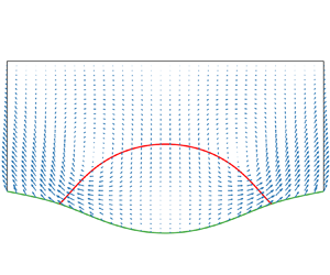
Several snapshots of the system at different times are shown in figure 3 for the wetting case and figure 4 for the non-wetting case. In both cases, the sheet, which is flat initially, is deformed. A pair of vortices in the velocity field form along with the evolution of the fluid interface. In the wetting case, outward velocities are generated at the contact lines driving the droplet to spread on the sheet. In the non-wetting case, the contact lines retreat with inward velocities.

Figure 3. The interface profiles and the fluid velocity for the wetting case ( $\theta _Y={\rm \pi} /3$): (a)
  $t=0$,
  $\max _{{\boldsymbol x}\in \varOmega }|\boldsymbol {u}| = 0$; (b)
  $t=0.05$,
  $\max _{{\boldsymbol x}\in \varOmega }|\boldsymbol {u}| = 1.207$; (c)
  $t=0.2$,
  $\max _{{\boldsymbol x}\in \varOmega }|\boldsymbol {u}| = 0.478$; (d)
  $t=1.0$,
  $\max _{{\boldsymbol x}\in \varOmega }|\boldsymbol {u}| = 0.027$.

Figure 4. The interface profiles and the fluid velocity for the non-wetting case ( $\theta _Y=2{\rm \pi} /3$): (a)
  $t=0$,
  $\max _{{\boldsymbol x}\in \varOmega }|\boldsymbol {u}| = 0$; (b)
  $t=0.05$,
  $\max _{{\boldsymbol x}\in \varOmega }|\boldsymbol {u}| = 1.203$; (c)
  $t=0.2$,
  $\max _{{\boldsymbol x}\in \varOmega }|\boldsymbol {u}| = 0.130$; (d)
  $t=1.0$,
  $\max _{{\boldsymbol x}\in \varOmega }|\boldsymbol {u}| = 0.005$.
In figure 5(a,b), we show the curvature and in figure 5(c,d) the tension of the elastic sheet at different times. Both the curvature gradient and the tension exhibit a jump across the contact line. The magnitude of the tension decays to  $0$ as the system approaches the equilibrium. The insets of panels (c, d) show the gradient of the tension rescaled by the friction coefficient,
  $({1}/{\mu _i})|\boldsymbol {\nabla }_s\nu |$, along the sheet. We observe that the rescaled gradient is continuous, though the tension itself has a jump at the contact line. Also the rescaled gradient of the tension attains the maximum at the contact line, indicating maximum slip occurs there according to (3.28b).

Figure 5. (a,b) Curvature and (c,d) tension of the sheet at different times: (a) curvature,  $\theta _Y={\rm \pi} /3$; (b) curvature,
  $\theta _Y=2{\rm \pi} /3$; (c) tension,
  $\theta _Y={\rm \pi} /3$; (d) tension,
  $\theta _Y=2{\rm \pi} /3$. The insets in panels (c,d) are plots of
  $({1}/{\mu _i})|\boldsymbol {\nabla }_s\nu |$.
In figure 6(a), we plot the total energy and in figure 6(b) the bending energy against time. The total energy decays in time, as expected from the energy dissipation property of the dynamical system. The bending energy, however, shows a rapid increase as a result of the deformation of the sheet at an initial stage.

Figure 6. (a) Rescaled energy  $\mathcal {E}(t)/\mathcal {E}(0)$ versus time; (b) bending energy,
  $\mathcal {E}_w(t)=({c_b}/{2})\int _{\varXi (t)}\kappa ^2\,\mathrm {d}s$, versus time.
Following the dynamics, the system eventually relaxes to the equilibrium state (steady state). In figure 7, we show the steady-state profiles of the interface and the sheet with large and small bending modulus. In the stiff case ( $c_b=100$), the sheet remains nearly flat and the droplet has the usual shape of a circular arc with the contact angle satisfying the Young–Dupré equation (panels a,c). In the soft case (
 $c_b =0.001$), the sheet is significantly deformed (panels b,d). Its curvature undergoes a rapid change near the contact line (the inner region) but is nearly constant away from the contact line (the outer region). The size of the inner region is of the order of
  $\sqrt {c_b}$. These results agree with the asymptotic solutions discussed in § 2, as shown in panels (c,d), where we overlay the asymptotic solutions in the outer region.

Figure 7. The steady-state profiles of the fluid interface and the sheet: (a)  $\theta _Y={\rm \pi} /3$,
  $c_b=100$; (b)
  $\theta _Y={\rm \pi} /3$,
  $c_b=0.001$; (c)
  $\theta _Y=2{\rm \pi} /3$,
  $c_b=100$; (d)
  $\theta _Y=2{\rm \pi} /3$,
  $c_b=0.001$. The insets in panels (b,d) are plots of the sheet curvature
  $\kappa$. The overlayed black dashed curves in panels (c,d) are plots of the asymptotic solutions in the stiff (panel c) and soft (panel d) limits.
Furthermore, we measured the apparent contact angles formed by the three interfaces in the outer region (see figure 7b). Specifically, we fit the fluid interface using a constant-curvature (circular) arc. The arc goes through the apex of the interface and also fits the curvature of the interface there. Similarly, we fit the sheet under the droplet using a circular arc through the middle point of the sheet. The two arcs intersect at an apparent contact line. The sheet outside the droplet is fitted using a horizontal line through the apparent contact line. The apparent contact angles are then measured between these fitting curves at the apparent contact line. The results are reported in table 1 for various small bending modulus. We see that, though the real contact angle satisfies the Young–Dupré equation, the apparent angles converge to the values predicted by Neumann's law (2.4) as the bending modules decrease towards 0. This agrees with the asymptotic results in Zhang et al. (Reference Zhang, Yao and Ren2020).


5. Application: bendotaxis
In this application, we consider the dynamics of a droplet driven by bendotaxis. The setup of the system is shown in figure 8. A droplet is confined between two semi-infinite elastic sheets in two dimensions. The left ends of the sheets are fixed at  $(0, \pm B_y)$. An interesting phenomenon observed in experiments is that the droplet migrates spontaneously along the channel from the fixed end to the free end (left to right), regardless of the wetting property of the droplet (Bradley et al. Reference Bradley, Box, Hewitt and Vella2019). Here, we use the model derived in § 3 to simulate the coupled dynamics of the sheets and the droplet.

Figure 8. Setup of bendotaxis. A liquid droplet is placed in a channel bounded by two semi-infinite elastic sheets. The left ends of the sheets are fixed at  $(0, \pm B_y)$.
The droplet is formed by a Newtonian fluid and outside of the droplet is a vacuum. The dynamics is governed by the equations in § 3.3. At the left end  $x=0$ where the sheets are fixed, we impose the clamped boundary conditions
 \begin{equation} \dot{\boldsymbol{q}} = 0, \quad \frac{\partial y}{\partial \xi} = 0, \end{equation}
where  ${\boldsymbol {q}}(\xi, t) = (x, y)$. For convenience of the simulation, we use
  $x$ to parametrize the sheets,
  ${\boldsymbol {q}} = (x, y(x, t))$. We truncate the system on the right at
  $x=B_x$ and impose the natural boundary conditions for the sheets as given in (4.3). These conditions allow material points of the sheets to cross the boundary at
  $x=B_x$, thus, although the sheets are inextensible, their lengths over the domain
  $[0, B_x]$ are not fixed. Furthermore, since the system is symmetric about the centreline of the channel at
  $y=0$, we only carry out the computation in the lower half of the channel and impose the symmetry conditions along
  $y=0$,
 \begin{gather} \frac{\partial u_1}{\partial y} = 0, \quad u_2 = 0, \end{gather}
 \begin{gather}\theta_l = \theta_r = \frac{\rm \pi}{2}, \end{gather}
where  $\boldsymbol {u}=(u_1, u_2)$ is the fluid velocity, and
  $\theta _l$ and
  $\theta _r$ are the angles between the fluid–vacuum interfaces and the centreline
  $y=0$.
Given an initial configuration of the system, we compute the dynamics by solving the governing equations in § 3.3 together with the boundary conditions (5.1a,b) and (5.2) using the finite element method. Specifically, we compute the fluid velocity, the fluid pressure, the profile of the sheet and its tension, as well as the fluid–vacuum interfaces. Below, we present the numerical results and investigate the mechanism of bendotaxis. We also study the effects of the wettability and bending modulus of the sheets on the dynamics. In all simulations, the initial configuration of the system is prepared by holding the sheets straight while letting the droplet relax until reaching equilibrium with the sheets. Then we release the sheets (except their fixed left ends) and let the system evolve. The contact lines of the initial relaxed droplet are located at  $x_l=2$ and
  $x_r=6$, respectively. Other parameters are chosen as
  $B_x = 10,\ B_y = 0.5,\ \mu _{\varLambda }=0.1, \ l_s = 0.1, \ Ca=0.1$.
We first report numerical results for a wetting case with  $\gamma _1=0.3,\ \gamma _2=1, \cos \theta _Y=0.7$ and a non-wetting case with
  $\gamma _1=1,\ \gamma _2=0.3,\ \cos \theta _Y=-0.7$. The bending modulus
  $c_b$ is
  $5\times 10^3$ in both cases. To examine the deflection of the sheets, we plot the time history of the width
  $w(t)$ of the channel measured at its free end in figure 9. The sheets deflect inwards leading to a narrower opening at the free end in the wetting case, while the opposite is observed in the non-wetting case. The deflection is more significant in the wetting case. Furthermore, a rapid deflection of the sheets occurs at the beginning of the process (
 $t\lesssim 0.3$) in both cases. As shown in figures 10 and 11, the droplet remains nearly still in this stage. Droplet motion only occurs in the later stage (
 $t\gtrsim 0.3$) as a result of the sheet deflection.

Figure 9. The channel width  $w(t)$ at the free end versus time. The two curves correspond to the wetting case (lower) and non-wetting case (upper), respectively.

Figure 10. Snapshots of the wetting case ( $\cos \theta _Y=0.7$). The fluid velocity and pressure are shown using arrows and colour code, respectively: (a)
  $t=0.05$; (b)
  $t=0.3$; (c)
  $t=1.0$; (d)
  $t=15.0$.

Figure 11. Snapshots of the non-wetting case ( $\cos \theta _Y=-0.7$). The fluid velocity and pressure are shown using arrows and colour code, respectively: (a)
  $t=0.05$; (b)
  $t=0.3$; (c)
  $t=1.0$; (d)
  $t=15.0$; (e)
  $t=90.0$.
The sheet deflection is mainly caused by the Laplace pressure of the droplet. In the wetting case, the pressure inside the droplet is negative (assuming zero pressure for the vacuum), which causes the sheets to deflect inwards. In contrast, in the non-wetting case, the pressure of the droplet is positive, resulting in an outward sheet deflection. In addition, the capillary force at the contact line also contributes to the sheet deflection. The capillary force pulls the sheets inwards, which facilitates the inward deflection in the wetting case, but impedes the outward deflection in the non-wetting case. This explains the larger deflection in the wetting case as observed in figure 9.
The deflection of the sheets results in a net force that drives the droplet towards the free end of the channel. Specifically, three forces mainly contribute to the droplet motion: (1) the bending force  $\boldsymbol {f}_b = ({c_b}/{Ca})(\Delta _s\kappa +\tfrac {1}{2}\kappa ^3){\boldsymbol n}$; (2) the sheet curvature force
  $\boldsymbol {f}_t = ({1}/{Ca})(\nu -\gamma _1)\kappa {\boldsymbol n}$; and (3) the forces at the left and right contact lines
  $\boldsymbol {F}_{\varLambda _l, \varLambda _r} = ({\gamma _3}/{Ca})\boldsymbol {m}_3$. For parameters used in the current simulation, we found that the force
  $\boldsymbol {f}_t$ due to the sheet tension is negligible compared to the other two forces. In figure 12, we show the horizontal component of the bending force at
  $t=0.3$,
  $\boldsymbol {f}_b\boldsymbol {\cdot } \boldsymbol {e}_1$, where
  $\boldsymbol {e}_1 = (1, 0)$. In both the wetting and non-wetting cases, the force has a rightward component, driving the droplet towards the free ends. The larger sheet deflection in the wetting case results in a larger bending force and consequently a faster droplet motion. The horizontal component of the contact line force,
  $(\boldsymbol {F}_{\varLambda _1}+\boldsymbol {F}_{\varLambda _2})\boldsymbol {\cdot }\boldsymbol {e}_1$, equals
  $0.147$ in the wetting case and
  $-0.0763$ in the non-wetting case at
  $t=0.3$. The opposite sign is due to the opposite direction of the sheet deflection in the two cases. As a result, the rightward droplet motion is further enhanced by the contact line force in the wetting case but impeded in the non-wetting case.

Figure 12. The horizontal component of the bending force,  $\boldsymbol {f}_b\boldsymbol {\cdot } \boldsymbol {e}_1$, along the sheet at
  $t = 0.3$. The two curves correspond to the wetting case (upper) and non-wetting case (lower), respectively.
To further examine the effects of wettability and stiffness of the sheets on the droplet dynamics, we carried out simulations with various contact angle  $\theta _Y$ and bending modulus
  $c_b$. The numerical results are summarized in figure 13(a), where we plot the dynamics of the right (advancing) contact point
  $x_r$. After rescaling the time by
 \begin{equation} t\rightarrow A(\cos\theta_Y, c_b)\boldsymbol{\cdot} t, \end{equation}
where  $A$ depends on
  $\cos \theta _Y$ and
  $c_b$, the data points for
  $({1}/{x_r(0)}-{1}/{x_r(t)})$ collapse into a master line with slope one. This shows that
 \begin{equation} x_r(t) = \frac{1}{\dfrac{1}{x_r(0)}-A t}. \end{equation}
The deviation of data points from this master line is mainly due to the large deflection of the sheets; in fact, in the case of  $\cos \theta _Y =0.9$ and
  $c_b =5000$, the free end of the channel is nearly closed when the droplet is close to that end, as shown in figure 13(d). Reducing the droplet size leads to smaller sheet deflection, in which case, a better agreement with the master line is observed (see the data points marked by ‘’).

Figure 13. (a) The dynamics of a droplet driven by bendotaxis with different contact angle  $\theta _Y$ and different bending modulus
  $c_b$. The data points marked by ‘’ are for a smaller droplet, whose size is one half that of the droplet in all other simulations. The dashed line has slope 1. (b) Doubly logarithmic plot of the coefficient
  $A$ versus
  $|\cos \theta _Y|$, where
  $c_b = 5000$. (c) Doubly logarithmic plot of coefficient
  $A$ versus
  $c_b$. (d) Configurations of the two systems with
  $\cos \theta _Y=0.9$ and
  $c_b = 5000$ (marked by ‘
 $\square$’ and ‘’ in panel a) at
  $At = 0.024$. The droplet in blue is half the size of that one in red.
The asymptotic relation (5.4) has been derived for small droplets under the lubrication approximation (Bradley et al. Reference Bradley, Box, Hewitt and Vella2019). There, the fluid interface was assumed to have a circular profile, and the contact angle was equal to the equilibrium Young's angle. It was shown that  $A \propto |\cos \theta _Y|^2/c_b$. The dependence of
  $A$ on
  $\theta _Y$ and
  $c_b$ obtained from the current numerical results is shown in figure 13(b,c). While the inverse proportionality relation of
  $A$ with the bending modulus
  $c_b$ agrees with the asymptotic result, discrepancies are observed for the relation with
  $\cos \theta _Y$. First of all, we find that
  $A$ is asymmetric about
  $\cos \theta _Y$. With the same value of
  $|\cos \theta _Y|$,
  $A$ is larger in the wetting case than in the non-wetting case. A larger value of
  $A$ corresponds to a faster droplet motion. Second, we observe that
  $A \propto |\cos \theta _Y|^\alpha$, where
  $\alpha$ is slightly less than
  $2$ in the wetting case but larger than
  $2$ in the non-wetting case. We believe that these discrepancies are mainly due to the contribution of the capillary force at the contact line, which was not fully taken into account in the previous asymptotic results. The capillary force of wetting droplets induces larger sheet deflections and consequently faster droplet motions. In addition, the finite droplet size also contributes to the discrepancies.
6. Conclusion
In this work, we considered the dynamics of a moving contact line on an elastic sheet. Based on generalized thermodynamics, we derived a hydrodynamic model, in particular, the necessary boundary conditions on the sheet and at the moving contact line. These boundary conditions can be interpreted as the balance of various forces. They were obtained by analysing the different energy dissipation mechanisms, in which the relevant fluxes and their corresponding forces were identified. The resulting model obeys an energy law, where the total energy of the dynamical system dissipates via the viscous force in the bulk fluids and the friction forces on the fluid–sheet interface and at the moving contact line.
The boundary conditions are summarized as follows. In the tangential direction of the sheet, the boundary conditions are given by the balance of the fluid shear stress with the friction force and the gradient of the sheet tension, respectively. The friction force is due to the slip between the fluids and the sheet. In the normal direction of the sheet, the boundary condition is given by the balance of the fluid normal stress with the bending force and the curvature force of the sheet. At the moving contact line, in the tangential direction to the sheet, the Young stress of the fluid interface is balanced by the friction force and the jump of the sheet tension, respectively. Here the Young stress refers to the capillary force arising from the deviation of the dynamic contact angle from the equilibrium angle, and the friction force is due to the motion of the contact line relative to the sheet. In the normal direction to the sheet, the capillary force of the fluid interface balances with the jump of the gradient of the sheet curvature. These force balances, together with the kinematic and inextensibility conditions, form the complete boundary conditions on the sheet for the hydrodynamic model.
Using this model, we numerically studied the relaxation dynamic of droplets on elastic sheets and the droplet motion driven by bendotaxis in a channel bounded by elastic sheets. In both applications, the full hydrodynamic model provided detailed information on the respective physical process. In addition to the usual hydrodynamic quantities such as the fluid velocity field and pressure, the interface and sheet profiles, we also obtained the dynamic contact angle, the slip velocity, the tension of the sheet, etc. This allowed us to better understand the dynamical processes as compared to simplified models (e.g. thin-film models).
For the relaxation dynamics of droplets on elastic sheets, we simulated two types of systems, one in the wetting case and the other in the non-wetting case. The numerical results verified the energy decay property of the model. The profiles of the fluid interface and the sheet at the steady state agreed well with the asymptotic solutions derived in an earlier work (Zhang et al. Reference Zhang, Yao and Ren2020).
For the motion of a droplet driven by bendotaxis, we simulated the dynamical process and investigated the mechanism of the droplet motion. We identified two stages in the dynamical process, one being an initial period in which the sheets were deflected, and the other being the subsequent period in which droplet transport occurred. We found that the sheet deflection was caused by the Laplace pressure of the droplet and the capillary force of the fluid interface. The latter always pulled the sheets inwards, thus it enhanced the inward deflection in the wetting case but hindered the outward deflection in the non-wetting case. A larger sheet deflection resulted in larger bending forces and consequently a faster droplet motion. Our numerical results also showed that the motion of a wetting (respectively non-wetting) droplet was further enhanced (respectively hindered) by the combined contact line forces. Furthermore, we examined the effect of the droplet wettability and sheet stiffness on the dynamics. After a proper rescaling of time, the dynamics of the various systems collapsed into a universal line.
The two applications demonstrate that our model is able to model complex fluid–sheet interactions in the presence of moving contact lines. With this model, we are in a position to systematically study many interesting elastocapillary problems, such as capillary rise in elastic tubes, spontaneous wrapping of liquid drops by elastic sheets, bubble dynamics on porous polymer films, etc. The model can be generalized to three dimensions in a straightforward manner, where the boundary and contact line conditions will take similar forms as in two dimensions. Simulations for 3-D problems become more challenging in view of the requirements for quality mesh generation and efficient solvers. We will leave these problems to the future work.
Acknowledgments
We thank an anonymous reviewer for helpful discussions on the arguments leading to the force balance equations (3.15), (3.16) and (3.21).
Funding
The work of W.R. was supported in part by Singapore MOE Academic Research Fund Tier 2 (Project No. MOE-T2EP20120-0009) and NSFC (No. 11871365). The work of Z.Z. was partially supported by the NSFC grant (No. 11731006, No. 12071207), NSFC Tianyuan-Pazhou grant (No. 12126602), the Guangdong Basic and Applied Basic Research Foundation (2021A1515010359), and the Guangdong Provincial Key Laboratory of Computational Science and Material Design (No. 2019B030301001).
Declaration of interests
The authors report no conflict of interest.
Appendix A. Variation of the Willmore energy
We provide some results from differential geometry that were used to compute the variation of the energies in § 3. Let  ${\boldsymbol {q}}(\xi,t)=(x(\xi,t),y(\xi,t))$ denote a curve
  $\varGamma$ parametrized by
  $\xi \in D_{\xi }$. The tangent, normal and curvature of the curve are respectively given by
 \begin{equation} \left. \begin{gathered}
\boldsymbol{\tau}=\frac{1}{|\partial_{\xi}{\boldsymbol{q}}|}\left(\frac{\partial
x}{\partial \xi}, \frac{\partial y}{\partial \xi}\right),
\\ {\boldsymbol
n}=\frac{1}{|\partial_{\xi}{\boldsymbol{q}}|}\left(\frac{\partial
y}{\partial \xi}, -\frac{\partial x}{\partial \xi}\right),
\\
\kappa=\boldsymbol{\nabla}_s\boldsymbol{\cdot}{\boldsymbol
n}=\frac{1}{|\partial_{\xi}{\boldsymbol{q}}|^3}\left(\frac{\partial
x}{\partial \xi}\frac{\partial^2y}{\partial
{\xi}^2}-\frac{\partial y}{\partial
\xi}\frac{\partial^2x}{\partial {\xi}^2}\right).
\end{gathered} \right\} \end{equation}
\begin{equation} \left. \begin{gathered}
\boldsymbol{\tau}=\frac{1}{|\partial_{\xi}{\boldsymbol{q}}|}\left(\frac{\partial
x}{\partial \xi}, \frac{\partial y}{\partial \xi}\right),
\\ {\boldsymbol
n}=\frac{1}{|\partial_{\xi}{\boldsymbol{q}}|}\left(\frac{\partial
y}{\partial \xi}, -\frac{\partial x}{\partial \xi}\right),
\\
\kappa=\boldsymbol{\nabla}_s\boldsymbol{\cdot}{\boldsymbol
n}=\frac{1}{|\partial_{\xi}{\boldsymbol{q}}|^3}\left(\frac{\partial
x}{\partial \xi}\frac{\partial^2y}{\partial
{\xi}^2}-\frac{\partial y}{\partial
\xi}\frac{\partial^2x}{\partial {\xi}^2}\right).
\end{gathered} \right\} \end{equation}
In addition, we have  $\partial _{\xi }\boldsymbol {\tau } = -|\partial _{\xi }{\boldsymbol {q}}|\kappa {\boldsymbol n}$ and
  $\partial _{\xi }{\boldsymbol n}=|\partial _{\xi }{\boldsymbol {q}}|\kappa \boldsymbol {\tau }$.
Let  $\mathcal {D}$ be a differential operator. We have
 \begin{equation} \mathcal{D}|\partial_{\xi}{\boldsymbol{q}}| = \frac{1}{|\partial_{\xi}{\boldsymbol{q}}|}\frac{\partial{\boldsymbol{q}}}{\partial \xi}\boldsymbol{\cdot}\frac{\partial\mathcal{D}{\boldsymbol{q}}}{\partial \xi} = (\boldsymbol{\nabla}_s\boldsymbol{\cdot}\mathcal{D}{\boldsymbol{q}})|\partial_{\xi}{\boldsymbol{q}}|, \end{equation}
where  $\boldsymbol {\nabla }_s = ({1}/{|\partial _{\xi }{\boldsymbol {q}}|^2})({\partial {\boldsymbol {q}}}/{\partial \xi })({\partial }/{\partial \xi })$ is the surface gradient. For a given function
  $f$ defined on the curve
  $\varGamma$, we have
 \begin{equation} \frac{\mathrm{d}}{\mathrm{d}t}\int_{\varGamma} f({\boldsymbol{q}},t) \,\mathrm{d}s = \int_{\varGamma}\left(\frac{\partial f}{\partial t}+\dot{\boldsymbol{q}}\boldsymbol{\cdot}\boldsymbol{\nabla} f+(\boldsymbol{\nabla}_s\boldsymbol{\cdot}\dot{\boldsymbol{q}})f\right)\,\mathrm{d}s, \end{equation}
where we have used (A2) with  $\mathcal {D}={\partial }/{\partial t}$.
The surface divergence theorem for a vector function  $\boldsymbol {F}(\xi )$ defined on
  $\varGamma$ reads
 \begin{align} \int_{\varGamma}\boldsymbol{\nabla}_s\boldsymbol{\cdot}\boldsymbol{F} \,\mathrm{d}s &= \int_{D_{\xi}}\boldsymbol{\tau}\boldsymbol{\cdot}\partial_{\xi}\boldsymbol{F} \,\mathrm{d}\xi\nonumber\\ &=(\boldsymbol{F}\boldsymbol{\cdot}\boldsymbol{m})\Big|_{\partial\varGamma}-\int_{D_{\xi}}\boldsymbol{F}\boldsymbol{\cdot}\partial_{\xi}\boldsymbol{\tau} \,\mathrm{d}\xi\nonumber\\ &=(\boldsymbol{F}\boldsymbol{\cdot}\boldsymbol{m})\Big|_{\partial\varGamma}+\int_{\varGamma}\kappa\boldsymbol{F}\boldsymbol{\cdot}{\boldsymbol n} \,\mathrm{d}s, \end{align}
where  $\boldsymbol {m}$ is the outward conormal of
  $\varGamma$.
Applying the differential operator  $\mathcal {D}$ on the curvature
  $\kappa$, we obtain
 \begin{align} \mathcal{D}\kappa &= \mathcal{D}(\boldsymbol{\nabla}_s\boldsymbol{\cdot}{\boldsymbol n}) = \mathcal{D}\left(\frac{\boldsymbol{\tau}}{|\partial_{\xi}{\boldsymbol{q}}|}\boldsymbol{\cdot}\partial_{\xi}{\boldsymbol n}\right)\nonumber\\ &=\frac{\mathcal{D}\boldsymbol{\tau}}{|\partial_{\xi}{\boldsymbol{q}}|}\boldsymbol{\cdot}\partial_{\xi}{\boldsymbol n}+\mathcal{D} \left(\frac{1}{|\partial_{\xi}{\boldsymbol{q}}|}\right)\boldsymbol{\tau}\boldsymbol{\cdot}\partial_{\xi}{\boldsymbol n} +\frac{\boldsymbol{\tau}}{|\partial_{\xi}{\boldsymbol{q}}|}\boldsymbol{\cdot}\frac{\partial}{\partial\xi}(\mathcal{D}{\boldsymbol n})\nonumber\\ &=\left[-(\boldsymbol{\nabla}_s\boldsymbol{\cdot}(\mathcal{D}{\boldsymbol{q}}))(\boldsymbol{\nabla}_s\boldsymbol{\cdot}{\boldsymbol n}) +\frac{1}{|\partial_{\xi}{\boldsymbol{q}}|^2}\frac{\partial}{\partial\xi}(\mathcal{D}{\boldsymbol{q}})\boldsymbol{\cdot}\partial_{\xi}{\boldsymbol n} \right] -\boldsymbol{\nabla}_s\boldsymbol{\cdot}(\mathcal{D}{\boldsymbol{q}})\frac{\boldsymbol{\tau}}{|\partial_{\xi}{\boldsymbol{q}}|}\boldsymbol{\cdot}\partial_{\xi}{\boldsymbol n}\nonumber\\ &\quad + \boldsymbol{\nabla}_s\boldsymbol{\cdot}\left[- \boldsymbol{\nabla}_s(\mathcal{D}{\boldsymbol{q}}\boldsymbol{\cdot}{\boldsymbol n})+\frac{\boldsymbol{\tau}}{|\partial_{\xi}{\boldsymbol{q}}|}(\mathcal{D}{\boldsymbol{q}}\boldsymbol{\cdot}\partial_{\xi}{\boldsymbol n})\right]\nonumber\\ &={-}\Delta_s(\mathcal{D}{\boldsymbol{q}}\boldsymbol{\cdot}{\boldsymbol n})-\kappa(\boldsymbol{\nabla}_s\boldsymbol{\cdot}(\mathcal{D}{\boldsymbol{q}}))+\boldsymbol{\nabla}_s\boldsymbol{\cdot}[\boldsymbol{\tau}(\kappa\boldsymbol{\tau}\boldsymbol{\cdot}(\mathcal{D}{\boldsymbol{q}}))]\nonumber\\ &={-}\Delta_s(\mathcal{D}{\boldsymbol{q}}\boldsymbol{\cdot}{\boldsymbol n})-(\mathcal{D}{\boldsymbol{q}}\boldsymbol{\cdot}{\boldsymbol n})\kappa^2+\boldsymbol{\nabla}_s\kappa\boldsymbol{\cdot}(\mathcal{D}{\boldsymbol{q}}), \end{align}
where we have used  $\partial _{\xi }\boldsymbol {\tau }=-|\partial _{\xi }{\boldsymbol {q}}|\kappa {\boldsymbol n}$ in the last step.
Finally, the time derivative of the Willmore energy of  $\varGamma$ is given by
 \begin{align} \frac{\mathrm{d}}{\mathrm{d}t} \int_{\varGamma}\kappa^2 \,\mathrm{d}s &=\int_{\varGamma}(2\kappa\frac{\partial}{\partial t}\kappa+\kappa^2(\boldsymbol{\nabla}_s\boldsymbol{\cdot}\dot{\boldsymbol{q}}))\,\mathrm{d}s\nonumber\\ &=\int_{\varGamma}-2\kappa\Delta_s(\dot{\boldsymbol{q}}\boldsymbol{\cdot}{\boldsymbol n})-2(\dot{\boldsymbol{q}}\boldsymbol{\cdot}{\boldsymbol n})\kappa^3+\boldsymbol{\nabla}_s\boldsymbol{\cdot}(\kappa^2\dot{\boldsymbol{q}})\,\mathrm{d}s\nonumber\\ &= 2\int_{\varGamma}(-\dot{\boldsymbol{q}}\boldsymbol{\cdot}{\boldsymbol n})(\Delta_s\kappa+\frac{1}{2}\kappa^3) \,\mathrm{d}s\nonumber\\ &\quad +2\left(-\kappa\boldsymbol{m}\boldsymbol{\cdot}\boldsymbol{\nabla}_s (\dot{\boldsymbol{q}}\boldsymbol{\cdot}{\boldsymbol n})+(\boldsymbol{m}\boldsymbol{\cdot}\boldsymbol{\nabla}_s\kappa) (\dot{\boldsymbol{q}}\boldsymbol{\cdot}{\boldsymbol n})+\frac{1}{2}\kappa^2\dot{\boldsymbol{q}}\boldsymbol{\cdot}\boldsymbol{m}\right)\Big|_{\partial\varGamma}, \end{align}
where we have used (A3) with  $f=\kappa ^2$ in the first step, (A5) with
  $\mathcal {D}={\partial }/{\partial t}$ in the second step, and the divergence theorem (A4) as well as integration by parts in the last step.
Appendix B. Weak formulation of the model
In this appendix, we give the weak formulation of the model that was used to simulate the drop relaxation dynamics in § 4. We parametrize the fluid interface as  ${\boldsymbol {r}}(\zeta )$ where
  $\zeta \in [0,1]$ and the sheet as
  ${\boldsymbol {q}}(x) = (x, y(x))$ where
  $x \in [-1,1]$. The two contact lines of the droplet are located at
  ${\boldsymbol {r}}(0) =(x_l, y(x_l))$ and
  ${\boldsymbol {r}}(1) = (x_r, y(x_r))$.
We define the following respective function spaces for the fluid velocity, the fluid pressure and the sheet tension,
 \begin{gather} \mathbb{U} =\{\boldsymbol{\omega}\in [H^1(\varOmega)]^2,\ \boldsymbol{\omega}=\boldsymbol{0}\ \text{on }\varSigma_5\}, \end{gather}
 \begin{gather}\mathbb{P}=\left\{\varphi\in L^2(\varOmega),\ \int_{\varOmega}\varphi \,\mathrm{d}\boldsymbol{x}= 0\right\}, \end{gather}
 \begin{gather}V_{1} = H^1([x_l,x_r]), \quad V_{2} = \{g\in H^1([{-}1,x_l]\cup[x_r,1]),\ g({-}1)=g(1)=0\}. \end{gather}
We take the inner product of (3.26a) with  $\boldsymbol {\omega }\in \mathbb {U}$, (3.26b) with
  $\varphi \in \mathbb {P}$, (3.35) with
  $f\in H^1([-1,1])$, (3.32) with
  $g_1\in V_{1}$ and
  $g_2\in V_2$, and (3.27c) with
  $\boldsymbol {\psi } \in H^1([0,1])\times H^1_0([0,1])$. Furthermore, we take the inner product of
  $\kappa /|\partial _x{\boldsymbol {q}}|=\Delta _s y$ with
  $\beta \in H^1_0([-1,1])$. Using the interface and boundary conditions, we obtain the following equations:
 \begin{gather} -\left(p, \boldsymbol{\nabla}\boldsymbol{\cdot}\boldsymbol{\omega}\right)_{\varOmega}+\left(\eta(\boldsymbol{\nabla}\boldsymbol{u}+(\boldsymbol{\nabla}\boldsymbol{u})^{\rm T}),\ \boldsymbol{\nabla}\boldsymbol{\omega}\right)_{\varOmega}+\frac{1}{Ca}\left(\partial_s{\boldsymbol{r}}, \partial_s\boldsymbol{\omega}\right)_{\varSigma_3} \\ -\frac{1}{Ca}\left(\nu, \boldsymbol{\nabla}_s\boldsymbol{\cdot}\boldsymbol{\omega}\right)_{\varXi}+\frac{1}{Ca}\left(c_b\partial_s\left(\frac{\kappa}{|\partial_x{\boldsymbol{q}}|}\right)+\frac{3c_b}{2}\kappa^2\partial_sy-\gamma\partial_sy, \partial_s(|\partial_x{\boldsymbol{q}}|\boldsymbol{\omega}\boldsymbol{\cdot}{\boldsymbol n})\right)_{\varXi} \nonumber\\ +\,\frac{\gamma_1-\gamma_2}{Ca}\left((|\partial_x{\boldsymbol{q}}|\omega_1)|_{\varLambda_r} -\left(|\partial_x{\boldsymbol{q}}|\omega_1\right)|_{\varLambda_l}\right)=0, \quad \forall \boldsymbol{\omega}=(\omega_1,\omega_2)\in\mathbb{U}, \nonumber\\ \left(\boldsymbol{\nabla}\boldsymbol{\cdot}\boldsymbol{u},\ \varphi\right)_{\varOmega} = 0, \quad \forall \varphi\in\mathbb{P}, \end{gather}
 \begin{gather}\left(\frac{\partial y}{\partial t},\ f\right)_{\varXi}+\left(|\partial_x {\boldsymbol{q}}|\boldsymbol{u}\boldsymbol{\cdot}{\boldsymbol n},\ f\right)_{\varXi} = 0, \quad \forall f\in H^1([{-}1,1]), \end{gather}
 \begin{gather}\frac{l_s}{\mu_1}\left(\partial_s\nu,\ \partial_s g_1\right)_{\varSigma_1} + Ca\left(\boldsymbol{\nabla}_s\boldsymbol{\cdot}\boldsymbol{u},\ g_1\right)_{\varSigma_1} +\frac{1}{\mu_{\varLambda}}\left([\![\nu]\!]^1_2g_1\right)\Big|_{\varLambda}= 0, \quad \forall g_1\in V_1, \end{gather}
 \begin{gather}\frac{l_s}{\mu_2}\left(\partial_s\nu,\ \partial_s g_2\right)_{\varSigma_2} + Ca\left(\boldsymbol{\nabla}_s\boldsymbol{\cdot}\boldsymbol{u},\ g_2\right)_{\varSigma_2} -\frac{1}{\mu_{\varLambda}}\left([\![\nu]\!]^1_2g_2\right)\Big|_{\varLambda} = 0, \quad \forall g_2\in V_2, \end{gather}
 \begin{gather}\left(\dot{\boldsymbol{r}},\ \boldsymbol{\psi}\right)_{\varSigma_3} - \left(\boldsymbol{u}, \boldsymbol{\psi}\right)_{\varSigma_3} = 0, \quad \forall \boldsymbol{\psi} \in H^1([0,1])\times H^1_0([0,1]), \end{gather}
 \begin{gather}\left(\frac{\kappa}{|\partial_x{\boldsymbol{q}}|},\ \beta\right)_{\varXi}+\left(\partial_s y,\ \partial_s\beta\right)_{\varXi} = 0, \quad \forall \beta\in H^1_0([{-}1,1]), \end{gather}
where  $w|_{\varLambda _l}$ and
  $w|_{\varLambda _r}$ denote the value of
  $w$ at the left and right contact lines, respectively;
  $\eta$ takes the value
  $\eta _1$ in
  $\varOmega _1$ and
  $\eta _2$ in
  $\varOmega _2$; and
  $\gamma$ takes the value
  $\gamma _1$ on
  $\varSigma _1$ and
  $\gamma _2$ on
  $\varSigma _2$. The operator
  $\partial _s$ represents
  $({1}/{|\partial _x{\boldsymbol {q}}|})({\partial }/{\partial x})$ on the sheet and
  $({1}/{|\partial _{\zeta }{\boldsymbol {r}}|})({\partial }/{\partial \zeta })$ on the fluid–fluid interface. The inner products in the above equations are defined as
 \begin{gather} \left(\boldsymbol{u},\ {\boldsymbol v}\right)_{\varOmega} = \sum_{i=1}^2\int_{\varOmega_i(t)} \boldsymbol{u}\boldsymbol{\cdot}{\boldsymbol v} \,\mathrm{d}\boldsymbol{x}, \end{gather}
 \begin{gather}\left(u,\ v\right)_{\varSigma_1} = \int_{x_l}^{x_r} u(x)v(x)|\partial_x{\boldsymbol{q}}| \,\mathrm{d}x, \end{gather}
 \begin{gather}\left(u,\ v\right)_{\varSigma_2} = \int_{{-}1}^{x_l} u(x)v(x)|\partial_x{\boldsymbol{q}}| \,\mathrm{d}x + \int_{x_r}^{1} u(x)v(x)|\partial_x{\boldsymbol{q}}| \,\mathrm{d}x, \end{gather}
 \begin{gather}\left(u,\ v\right)_{\varXi} = \left(u,\ v\right)_{\varSigma_1} + \left(u, v\right)_{\varSigma_2}, \end{gather}
 \begin{gather}\left(\boldsymbol{u},\ {\boldsymbol v}\right)_{\varSigma_3} = \int_{0}^{1} \boldsymbol{u}(\zeta)\boldsymbol{\cdot}{\boldsymbol v}(\zeta) |\partial_{\zeta}{\boldsymbol{r}}| \,\mathrm{d}\zeta. \end{gather}


 Open access