


1. Introduction
A closure model for the third-order velocity structure function  $\overline {(\delta u)^{3}}$ (
 $\delta u= u(x) - u(x+r)$, where
  $r$ is the spatial separation in the longitudinal direction
  $x$ and the overbar represents ensemble averaging; the time variable is dropped for convenience) was proposed to close the transport equation for the second-order moment velocity increment
  $\overline {( \delta u)^{2}}$, i.e. the the Kármán–Howarth equation (Kármán & Howarth Reference Kármán and Howarth1938), in homogeneous and isotropic turbulence or HIT (Djenidi & Antonia Reference Djenidi and Antonia2021). The model was shown to yield good agreement with experiments and direct numerical simulations (Djenidi & Antonia Reference Djenidi and Antonia2022).
In the present study we extend this model to the third-order mixed velocity–scalar structure function  $-\overline {(\delta u)( \delta \phi )^{2}}$ in order to solve the transport equation for the scalar structure function for HIT (
 $\phi$ is a scalar quantity). Such an equation can be written in the following form (e.g. Danaila et al. Reference Danaila, Anselmet, Zhou and Antonia1999):
 \begin{equation} -\overline{(\delta u)( \delta \phi)^{2}} +2\alpha \frac{\partial{\overline{(\delta \phi)^{2}}}}{\partial r} -\frac{1}{r^{2}}\int^{r}_0 s^{2} \frac{\partial {\overline{(\delta \phi)^{2}}}}{\partial t} \, {{\rm d}}s = \frac{4}{3} \overline{\epsilon_{\phi}} r. \end{equation}
The quantity  $\overline {(\delta \phi )^{2}}= \overline {(\phi (x) - \phi (x+r))^{2}}$ (which we denote
  $S_{\phi ^{2}}$ for convenience; also, since
  $\overline {(\delta \phi )^{2}}$ is a function of
  $r$ one should perhaps write
  $\overline {(\delta _r \phi )^{2}}$ or
  $S_{r,\phi ^{2}}$; however, we drop the subscript
  $r$ to avoid cumbersome notation) is the second-order moment of the scalar increment
  $\delta \phi$. On the left-hand side of (1.1), the first term is the unknown third-order mixed velocity–scalar structure function, the second term is the molecular diffusion and the third term represents the contributions associated with the large-scale motion. This latter term is absent from the well-known Yaglom equation as Yaglom (Reference Yaglom1949) assumed that
  $\overline {(\delta \phi )^{2}}$ is independent of time. On the right-hand side of (1.1),
  $\overline {\epsilon _{\phi }} = \alpha \overline {(\partial \phi /\partial x_i)^{2}}$ is the scalar variance dissipation rate, where
  $\alpha$ is the diffusivity of
  $\phi$; if the scalar quantity is twice the turbulent kinetic energy (
 $q^{2}=2k$), then
  $\overline {\epsilon _{q}}= \bar {\epsilon }= \nu \overline {(\partial u_i/\partial x_k)^{2}}$. While (1.1) was initially written for the second-order moment of the temperature increments, it is also valid for any (passive) scalar quantity.
Unlike its spectral counterpart (e.g. Yeh & Atta Reference Yeh and Atta1973; Monin & Yaglom Reference Monin and Yaglom1975), the term  $-\overline {(\delta u)( \delta \phi )^{2}}$ has received less attention in terms of modelling. Danaila, Antonia & Burattini (Reference Danaila, Antonia and Burattini2012) modelled that term as (
 $r^{2} \, {{\rm d}}S_{\phi ^{2}}/{{\rm d}}r)/\tau$, where
  $\tau$ is a characteristic time. Although the authors did not use the model to actually solve (1.1), they nevertheless showed, using experimental data of grid turbulence, that (
 $r^{2} \, {{\rm d}}S_{\phi ^{2}}/ {{\rm d}}r)/\tau$) captures the behaviour of
  $-\overline {(\delta u)( \delta \phi )^{2}}$ (temperature was used as the passive scalar) reasonably well. There is so far no reported attempt at solving (1.1). Most of the numerical studies on the passive scalar in HIT are carried out via direct numerical simulations (DNSs) or the eddy damped quasi-normal Markovian (EDQNM) approach. The former solve the Navier–Stokes equations coupled with the scalar equation (e.g. Bogucki, Domaradzki & Yeung Reference Bogucki, Domaradzki and Yeung1997; Antonia & Orlandi Reference Antonia and Orlandi2002; Yeung, Xu & Sreenivasan Reference Yeung, Xu and Sreenivasan2002; Watanabe & Gotoh Reference Watanabe and Gotoh2004; Yeung & Sreenivasan Reference Yeung and Sreenivasan2014; Gotoh & Watanabe Reference Gotoh and Watanabe2015; Shete & de Bruyn Kops Reference Shete and de Bruyn Kops2020; Buaria et al. Reference Buaria, Clay, Sreenivasan and Yeung2021a). Unfortunately DNSs are limited to relatively low/moderate Reynolds numbers and Prandtl (or Schmidt) numbers (
 $Pr= \nu /\alpha$) due to the limitations of computing power as high-Reynolds-number and high-Prandtl-number simulations require very high resolution (see references cited above). The EDQNM approach solves the evolution equations of the kinetic energy and scalar variance spectra (e.g. Briard & Gomez Reference Briard and Gomez2017a,Reference Briard and Gomezb), where the spectral energy and scalar transfer terms are modelled and can achieve high Reynolds and Prandtl numbers (e.g. Briard & Gomez Reference Briard and Gomez2016).
Therefore, the present study is a first attempt at solving (1.1) using a model for  $-\overline {(\delta u)( \delta \phi )^{2}}$. The derivation of the this model is described in § 2. In § 3, a self-similarity analysis is carried out to determine appropriate scaling variables to be used for normalising the solutions to (1.1). Results of solutions to the modelled equation (1.1) for
  $Pr = 0.7$ and 1 are compared with both DNS and experimental data in § 4 while exploratory predictions at various Reynolds and Prandtl numbers are carried out in § 5. Concluding remarks are provided in § 6.
2. The closure model
One can interpret  $(\delta u)(\delta \phi )^{2}$ as the transport of
  $(\delta \phi )^{2}$ by
  $\delta u$. We can then follow Djenidi & Antonia (Reference Djenidi and Antonia2020, Reference Djenidi and Antonia2021) and seek to model
  $S_{u\phi ^{2}}=-\overline {(\delta u)( \delta \phi )^{2}}$ in the form of a gradient type. We thus model
  $S_{u\phi ^{2}}$ using a gradient-type hypothesis with an eddy-viscosity model; the model expression for
  $S_{u\phi ^{2}}$ has the following form:
 \begin{equation} S_{u\phi^{2}} = \nu_{S_{u\phi^{2}}} \frac{\partial S_{\phi}}{\partial r},\end{equation}
where  $\nu _{S_{u\phi ^{2}}}$ is an eddy viscosity, for which an analytical expression is sought. Djenidi & Antonia (Reference Djenidi and Antonia2020, Reference Djenidi and Antonia2021) used the form (2.1) to close the transport equation for
  $S_{u^{2}}=\overline {(\delta u)^{2}}$ and proposed an expression for
  $\nu _{S_{u^{2}}}$ based on dimensional arguments. They wrote
 \begin{equation} \nu_{S_{u^{2}}}\sim u_r l_r,\end{equation}
where  $u_r$ and
  $l_r$ are velocity and length scales characterising the motion at a scale
  $r$. They assumed
  $u_r \sim (S_u^{2})^{1/2}$ and proposed to use
  $l_r \sim u_r^{3}/\bar {\epsilon } \sim (S_{u^{2}})^{3/2}/\bar {\epsilon }$, which leads to
 \begin{equation} \nu_{S_{u^{2}}}= C_{S_{u^{2}}} \frac{(S_{u^{2}})^{2}}{\bar{\epsilon}},\end{equation}
and obtained
 \begin{equation} S_{u^{3}} = C_{S_{u^{2}}} \frac{(S_{u^{2}})^{2}}{\bar{\epsilon}} \frac{\partial S_{u^{2}}}{\partial r},\end{equation}
where  $C_{S_{u^{2}}}$ is a constant to be determined. The authors showed that this model is unaffected by the intermittency of
  ${\epsilon }$. This is consistent with the fact that
  ${S_{u^{3}}}$ is expected not to be affected by such a phenomenon. The transport equation (1.1) is similar for the turbulent kinetic energy,
  $q^{2}$, and any other variance of a passive scalar,
  $\phi ^{2}$, when
  $Pr=1$, which suggests an analogy between
  $q^{2}$ and
  $\phi ^{2}$ (Fulachier & Antonia Reference Fulachier and Antonia1984; Abe, Antonia & Kawamura Reference Abe, Antonia and Kawamura2009; Antonia, Abe & Kawamura Reference Antonia, Abe and Kawamura2009). Using this analogy when
  $Pr=1$, we simply adopt the approach of Djenidi & Antonia (Reference Djenidi and Antonia2020, Reference Djenidi and Antonia2021) and write (2.1) as follows:
 \begin{equation} S_{u\phi^{2}}= C_{S_{u\phi^{2}}} \frac{(S_{q^{2}})^{2}}{\bar{\epsilon}} \frac{\partial S_{\phi^{2}}}{\partial r}, \end{equation}
where we use  $u_r \sim (S_{q^{2}})^{1/2}$; also note that
  $\bar {\epsilon } = \bar {\epsilon }_q$. Let us first consider the case where there is a range of scales (
 $\eta \ll r \ll L$, i.e. the inertial range) over which both the viscous dissipation term and large-scale term (the second and third terms on the left-hand side of (1.1)) can be neglected. We are then left with
 \begin{equation} C_{S_{u\phi^{2}}} \frac{(S_{q^{2}})^{2}}{\bar{\epsilon}} \frac{\partial S_{\phi^{2}}}{\partial r} = \frac{4}{3} \bar{\epsilon}_\phi r.\end{equation}
If  $\phi = q$ we then have
 \begin{equation} C_{S_{uq^{2}}} \frac{(S_{q^{2}})^{2}}{\bar{\epsilon}} \frac{\partial S_{q^{2}}}{\partial r}=\frac{4}{3} \bar{\epsilon} r.\end{equation}
Integrating and rearranging terms leads to
 \begin{equation} S_{q^{2}}= C_q (\bar{\epsilon} r)^{2/3},\end{equation}
with  $C_q = (2/C_{S_{uq^{2}}})^{1/3}$. Antonia et al. (Reference Antonia, Zhu, Anselmet and Ould-Rouis1996) showed that
  $C_q=(11/3)C_K$, where
  $C_K$ is the Kolmogorov constant in
  $S_{u^{2}}=C_K(\bar {\epsilon } r)^{2/3}$. Now taking
  $\phi = \theta$ (say the temperature fluctuation) leads to
 \begin{equation} C_{S_{u\theta^{2}}} \frac{(S_{q^{2}})^{2}}{\bar{\epsilon}} \frac{\partial S_{\theta^{2}}}{\partial r}=\frac{4}{3} \bar{\epsilon}_\theta r.\end{equation}
Assuming we are in the range of scales over which (2.8) is valid and the second and third terms on the left-hand side of (1.1) are also negligible when  $\phi = \theta$, we then have
 \begin{equation} C_{S_{u\theta^{2}}} \frac{C_q^{2} (\bar{\epsilon} r)^{4/3}}{\bar{\epsilon}} \frac{\partial S_{\theta^{2}}}{\partial r}=\frac{4}{3} \bar{\epsilon}_\theta r.\end{equation}
Integrating this expression leads to
 \begin{equation} S_{\theta^{2}}= C_\theta \bar{\epsilon}_\theta \bar{\epsilon}^{{-}1/3} r^{2/3},\end{equation}
where  $C_\theta = 2/(C_q^{2}C_{S_{u\theta ^{2}}})$ is a constant to be determined. Antonia et al. (Reference Antonia, Zhu, Anselmet and Ould-Rouis1996) estimated that
  $C_\theta = C_qR$, where
  $R= (\overline {\theta ^{2}}/\bar {\epsilon }_\phi )/(\overline {q^{2}}/\bar {\epsilon })$ is the dissipation time-scale ratio. Note that the constants
  $C_K$ and
  $C_\theta$ are not to be confused with their spectral counterparts (Sreenivasan Reference Sreenivasan1995, Reference Sreenivasan1996). Below we test the model and compare the results against available data. However, we need first to determine appropriate scaling parameters. This is addressed in § 3.
3. Scaling variables
Before we solve (1.1) where the closure model (2.5) is introduced, we first seek self-preservation (SP) solutions to (1.1) to allow us to determine appropriate scaling variables. We seek solutions in the following form:
 \begin{equation} S_{\phi^{2}} = \phi_*^{2}(t)f_{\phi}(r_{\phi}^{*}), \quad S_{u^{2}} = u_*^{2}(t)f_{u}(r_\phi^{*}), \quad S_{u \phi^{2}} = B_*(t)g_{\phi}(r_\phi^{*}),\end{equation}
with  $r_{\phi }^{*} = r/l_{\phi }(t)$, and
  $l_{\phi }(t), u_*(t)$ and
  $\phi _*(t)$ are the length, velocity and scalar scaling functions to be determined,
  $B_*(t)$ is a mixed scaling and
  $f_{\phi }$ and
  $f_u$ are dimensionless functions. For convenience, we hereafter drop the variable
  $t$. Let us introduce the mixed skewness increment
  $S(r)$ (
 $\equiv S_{u \phi ^{2}}/[S_{u^{2}}^{1/2}S_{\phi ^{2}}]$). If SP is satisfied,
  $S(r)$ has also the SP form
  $S(r) = c_{\phi }(t)H_\phi (r^{*}_{\phi })$. We thus can take
  $B_* = u_*\phi _*^{2}$. Substituting the form (3.1a–c) into (1.1) leads to the following equation if SP is satisfied:
 \begin{equation} -Re_{l_\phi} g_{\phi}(r_{\phi}^{*}) + 2f'_{\phi}(r_{\phi}^{*}) -\frac{l_{\phi}^{2}}{\alpha \phi_*^{2}} \frac{\partial \phi_*^{2}}{\partial t}\frac{\varGamma_{1,\phi}}{r_{\phi}^{*2}} + \frac{l_{\phi}}{\alpha} \frac{\partial l_{\phi}}{\partial t}\frac{\varGamma_{2,\phi}}{r_{\phi}^{*2}} = \frac{4}{3} \frac{\overline{\epsilon_{\phi}}l_{\phi}^{2}}{\alpha \phi_*^{2}} r_{\phi}^{*}, \end{equation}
and the constraints on the various scaling variables
 \begin{gather} C_1=Re_{l_\phi}, \end{gather}
 \begin{gather}C_2 = 2, \end{gather}
 \begin{gather}C_3=\frac{l_{\phi}^{2}}{\alpha \phi_*^{2}} \frac{\partial \phi_*^{2}}{\partial t}, \end{gather}
 \begin{gather}C_4=\frac{l_{\phi}}{\alpha} \frac{\partial l_{\phi}}{\partial t}, \end{gather}
 \begin{gather}C_5=\frac{\overline{\epsilon_{\phi}}l_{\phi}^{2}}{\alpha \phi_*^{2}} \end{gather}
(a prime denotes a derivative with respect to  $r_{\phi }^{*}$), where
  $Re_{l_{\phi }} =u_*l_{\phi }/\alpha$ is a scaling Reynolds number or Péclet number and
 \begin{equation} \varGamma_{1,\phi}= \int_0^{r_{\phi}^{*}} s_{\phi}^{*2}f_{\phi}\, {{\rm d}}s_{\phi}^{*2}, \quad \varGamma_{2,\phi}= \int_0^{r_{\phi}^{*}} s_{\phi}^{*3}f'_{\phi}\, {{\rm d}}s_{\phi}^{*2}.\end{equation}
Since  $C_2$ is a constant, then
  $C_1, C_3, C_4$ and
  $C_5$ are also constants and thus time-independent. Combining (3.4) and (3.7) (we multiplied the numerator and denominator of the latter by
  $u_*^{2}$) and using the definition of
  $Re_{l_{\phi }}$ yields
 \begin{equation} l_{\phi}=(\sqrt{C_5}C_1)^{1/2} \left(\frac{\alpha^{3}}{\overline{\epsilon_{\phi}}}\right)^{1/4} \left(\frac{\phi_*}{u_*}\right)^{1/2}.\end{equation}
Now, substituting (3.9) in (3.7) leads to
 \begin{equation} \phi_*=\left(\frac{C_1}{\sqrt{C_5}}\right)(\alpha \overline{\epsilon_{\phi}})^{1/2}\frac{1}{u_*}.\end{equation}
Let us first consider the turbulent kinetic energy as the passive scalar. Thus,  $S_{\phi ^{2}} = S_{q^{2}}$ and
  $\alpha = \nu, \phi _* = u_*$ and
  $\overline {\epsilon _{\phi }}= \bar {\epsilon }$ (the mean turbulent kinetic energy dissipation rate), and recognising that
  $\eta = (\nu ^{3}/\bar {\epsilon })^{1/4}$ and
  $v_K= (\nu \bar {\epsilon })^{1/4}$ (the Kolmogorov length and velocity, respectively), we can write
 \begin{equation} l_q = C_{l_q}\eta, \quad u_* = C_{u_*}v_K. \end{equation}
If we now consider that the passive scalar is the temperature, we have  $S_{\phi ^{2}} = S_{\theta ^{2}}$ and denote
  $\alpha$ a thermal diffusivity, for example. This leads to
 \begin{equation} l_{\theta} = C_{l_\theta} \eta_\theta \left(\frac{\theta_*}{u_*}\right)^{1/2},\quad \theta_* = C_{\theta_*} v_\theta^{2} \frac{1}{u_*},\end{equation}
where we define for convenience  $\eta _\theta = (\alpha ^{3}/\overline {\epsilon _\theta })^{1/4}$ and
  $v_\theta = (\alpha \overline {\epsilon _\theta })^{1/4}$.
Substituting the second expression of (3.12a,b) into the first expression and taking  $u_* =v_K$, we obtain
 \begin{equation} l_{\theta} = C_{l_\theta}C_{\theta_*}^{1/2} \frac{1}{Pr^{1/4}R_\epsilon^{1/4}} \eta_{\theta} = C_{l_\theta} C_{\theta_*}^{1/2} \frac{1}{Pr^{1/4}} \tilde{\eta}_{\theta},\end{equation}
where  $R_\epsilon =({\bar {\epsilon }}/{\overline {\epsilon _\theta }}), \tilde {\eta }_{\theta }= (\alpha ^{3}/\bar {\epsilon })^{1/4}$ and
  $Pr = \nu /\alpha$ is the Prandtl number. Hereafter and for convenience we use the notation
  $Pr$ independently of whether the scalar is the temperature or any other quantity different from
  $q$. Note that we can also write (3.13) as
 \begin{equation} l_{\theta} = C_{l_\theta}C_{\theta_*}^{1/2} \frac{1}{Pr^{1/2}} \left(\frac{\alpha^{2} \nu}{\bar{\epsilon}}\right)^{1/4} \end{equation}
or
 \begin{equation} l_{\theta} = C_{l_\theta}C_{\theta_*}^{1/2} \frac{1}{Pr} \eta.\end{equation}
 Now, we have for  $\theta _*$
 \begin{equation} \theta_* = C_{\theta_*} \frac{1}{v_K}v_\theta^{2}= C_{\theta_*} \frac{1}{Pr^{1/4} R_\epsilon^{1/4}} v_\theta. \end{equation}
The derivation of the scaling variables (3.11a,b) from the equations of motion has been already shown and discussed elsewhere (Djenidi, Antonia & Danaila Reference Djenidi, Antonia and Danaila2017). Several expressions for  $l_\theta$, based on dimensional arguments, have been formulated in the literature. For example, Oboukhov (Reference Oboukhov1949) and Corrsin (Reference Corrsin1951) obtained
 \begin{equation} l_{C} = \left(\frac{\alpha^{3}}{\bar{\epsilon}}\right)^{1/4},\end{equation}
which is simply  $\tilde {\eta }_{\theta }$, while Batchelor (Reference Batchelor1959) obtained
 \begin{equation} l_{B} = \left(\frac{\alpha^{2} \nu}{\bar{\epsilon}}\right)^{1/4}.\end{equation}
These length scales are related as follows:
 \begin{equation} l_{C} = \frac{1}{Pr^{1/4}} l_{B}.\end{equation}
These two length scales are related to  $\eta$ as follows:
 \begin{gather} l_{C} = \frac{1}{Pr^{3/4}} \eta, \end{gather}
 \begin{gather}l_{B} = \frac{1}{Pr^{1/2}} \eta. \end{gather}
Finally we have the following relation:
 \begin{equation} l_{\theta} = C_{l_\theta}C_{\theta_*}^{1/2} \frac{1}{Pr^{1/4}} l_C= C_{l_\theta}C_{\theta_*}^{1/2} \frac{1}{Pr^{1/2}} l_B,\end{equation}
which shows how the present length scale,  $l_{\theta }$, issued from the SP analysis, relates to the empirical length scales of Corrsin and Batchelor,
  $L_C$ and
  $L_B$, respectively.
4. Numerical solutions
Let us for convenience denote hereafter the integral term in (1.1) as  $Z_\phi$. Using a linear forcing in the context of the Kármán–Howarth equation (Kármán & Howarth Reference Kármán and Howarth1938) expressed in terms of
  $S_{u^{2}}$, Lundgren (Reference Lundgren2003) showed that for stationary HIT the integral term corresponding to that in (1.1) can be replaced by a term,
  $Z_u$, of the following expression:
 \begin{equation} Z_{u}=\frac{2\bar{\epsilon}}{u'^{2}}\frac{1}{r^{4}}\int_0^{r} s^{4}S_{u^{2}}\, {{\rm d}}s, \end{equation}
and suggested that this forcing is equivalent to a uniform spectral forcing at all wavenumbers and can allow comparison with decaying HIT. By analogy to (4.1), and since we consider stationary HIT, we express  $Z_\phi (r)$ as follows:
 \begin{equation} Z_\phi=\frac{2\bar{\epsilon}_\phi}{\phi'^{2}}\frac{1}{r^{2}} \int_0^{r} s^{2}S_{\phi^{2}}\, {{\rm d}}s,\end{equation}
which gives the correct asymptotic limit  $Z_\phi = \frac {4}{3}\overline {\epsilon _\phi }r$ when
  $r/\eta \rightarrow \infty$. Substituting (2.5) and (4.2) in (1.1) we can solve the resulting equation in the following simple manner:
 \begin{equation} S_{\phi^{2}}(r+{\rm \Delta} r) = S_{\phi^{2}}(r) +\frac{\{ \frac{4}{3}\overline{\epsilon}_\phi r -Z_{\phi}\} {\rm \Delta} r}{2\alpha +C_{S_{u\phi^{2}}}[S_{q^{2}} (r)]^{2}/\bar{\epsilon}},\end{equation}
where the calculations start by evaluating the right-hand side of (4.3) at  $r= \eta +{\rm \Delta} r$ with the boundary condition
  $S_{\phi ^{2}}=({1}/{3\alpha })\overline {\epsilon _\phi }r^{2}$ at
  $r = \eta$, which is the correct solution of (1.1) in the viscous–diffusive range. The process is then repeated by increment of
  ${\rm \Delta} r$. Note that (4.3) requires knowledge of
  $S_{q^{2}}$ when
  $\phi ^{2}$ is any passive scalar variance different from the turbulent kinetic energy. Consequently, solutions of
  $S_{q^{2}}$ using (4.3) are obtained first before (4.3) is used again to obtain solutions of
  $S_{\phi ^{2}}$. In all calculations we follow Antonia et al. (Reference Antonia, Zhu, Anselmet and Ould-Rouis1996) and use
  $C_q = (11/3)C_K =7.3$, where we assume
  $C_K = 2$. For
  $C_\theta$ we use the value matching that corresponding to the data we used for comparison; that value varies from 2.8 to 4. A definitive value is yet to be determined, although it is thought that a value of 3.2 corresponds to the equivalent spectral constant which has a value of 0.4 (e.g. Monin & Yaglom Reference Monin and Yaglom1975). To perform the calculation we use the values of
  $\bar {\epsilon }, \overline {\epsilon _\theta }, q^{2}$ and
  $\theta ^{2}$ reported in the references we have used to compare to. This ensures similar values of the dissipation time-scale ratio
  $R$ between our calculations and those of the references. Note that for clarity we take
  $\phi = q$ when the scalar is the turbulent kinetic energy and
  $\phi = \theta$ for any other passive scalar.
We first test the calculations against large Taylor microscale Reynolds number ( $Re_\lambda =2 \times 10^{4},\ {\rm where}\ \lambda$ is the Taylor microscale) EDQNM simulations of decaying HIT with
  $Pr=1$ (Briard & Gomez Reference Briard and Gomez2017a). The results are reported in figure 1 which shows a comparison between the calculated distributions of
  $S_{\phi ^{2}}$ and
  $S_{u\phi ^{2}}$ with their EDQNM counterparts. There is generally good agreement between the present calculations and the EDQNM simulations. It should be pointed out that
  $S_{u\phi ^{2}}$ is calculated using (2.5) once the distribution of
  $S_{\phi ^{2}}$ is obtained with (4.3). Notice the relatively good agreement for
  $S_{\phi ^{2}}$ at small separations, i.e.
  $0 \leq r/\eta \leq 10$. This is remarkable considering that the model (2.5) is not in principle adequate for the region outside the scaling range, as indeed observed for
  $S_{u\phi ^{2}}$. The reason why the calculated distribution of
  $S_{\phi ^{2}}$ is not significantly affected by the relatively poor performance of the model
  $S_{u\phi ^{2}}$ at small separations relates to the fact that
  $S_{u\phi ^{2}}$ approaches zero at a faster rate than the viscous term (second term on the left-hand side of (1.1)). Indeed,
  $S_{u\phi ^{2}} \sim r^{3}$ while
  $\partial S_{\phi ^{2}}/\partial r \sim r$ as
  $r\rightarrow 0$. The model (2.5) behaves like
  $r^{5}$ as
  $r \rightarrow 0$, thus leaving the solutions for
  $S_{\phi ^{2}}$ practically unaffected. For large separations the model also performs imperfectly. But once again this is not critical since
  $S_{u\phi ^{2}}$ approaches zero and the integral term in (1.1) dominates the budget. One possible reason for the small difference between the present results and the EDQNM results at large separations may relate to the fact that the EDQNM does not use non-local transfers to solve Lin's equation. Altogether, figure 1 shows that (2.5) provides an adequate closure for (1.1). This is supported by figures 2 and 3 which show comparisons between the present calculations and both experimental data (grid turbulence, Mydlarski & Warhaft (Reference Mydlarski and Warhaft1998); wake, Antonia et al. (Reference Antonia, Zhu, Anselmet and Ould-Rouis1996); jet, Burattini, Antonia & Danaila (Reference Burattini, Antonia and Danaila2005)) and DNS data of forced HIT (Watanabe & Gotoh Reference Watanabe and Gotoh2004);
  $Pr= 0.71$ and 1 for the experiments and DNSs, respectively. The results indicate that the linear forcing represented by (4.2) is adequate for the scalar field and that it reproduces adequately the large-scale motion contributions in both decaying and forced turbulence. This is further reinforced by comparing the present calculations with the DNS results for HIT fed by a mean scalar gradient at
  $Pr=1$ (Gauding, Danaila & Varea Reference Gauding, Danaila and Varea2017) as seen in figure 4. We used values of
  $\bar {\epsilon }, \overline {\epsilon _\theta }, q^{2}$ and
  $\theta ^{2}$ reported in Gauding et al. (Reference Gauding, Danaila and Varea2017);
  $R$ varies from about 0.48 to 0.423 when
  $Re_\lambda$ varies from 88 to 529. There is very good agreement between the DNS results and the calculations.

Figure 1. Distributions of the second-order scalar structure function  $S_{\phi ^{2}}$ and mixed structure function
  $S_{u\phi ^{2}}$ for
  $Pr=1$ and
  $Re_\lambda =2 \times 10^{4}$. Symbols: EDQNM decaying turbulence (Briard & Gomez Reference Briard and Gomez2017a); lines: present calculations;
  $S_{\phi ^{2}}$ is calculated using (4.3) and
  $S_{u\phi ^{2}}$ is calculated using (2.5).

Figure 2. Distributions of the second-order temperature structure function  $S_{\phi ^{2}}$ (
 $\phi = \theta$) for
  $Pr=0.71$. Symbols: decaying grid turbulence (Mydlarski & Warhaft Reference Mydlarski and Warhaft1998); lines: present calculations;
  $S_{\phi ^{2}}$ is calculated using (4.3).

Figure 3. Distributions of the second-order structure function  $S_{\phi ^{2}}$ as a function of
  $r/l_{C}$. Symbols: measurements (
 $Pr = 0.7$) on centrelines of a cylinder wake at
  $Re_\lambda = 230$ (Antonia et al. Reference Antonia, Zhu, Anselmet and Ould-Rouis1996) and round jet flow at
  $Re_\lambda = 450$ (Burattini et al. Reference Burattini, Antonia and Danaila2005) and DNS of HIT,
  $Re_\lambda = 258$ and 427,
  $Pr=1$ (Watanabe & Gotoh Reference Watanabe and Gotoh2004); lines: calculations;
  $S_{\phi ^{2}}$ is calculated using (4.3).

Figure 4. Distributions of the second-order structure function  $S_{\phi ^{2}}$ as a function of
  $r/l_{C}$. Symbols: DNS of HIT with a scalar mean gradient,
  $Re_\lambda = 88$ (circles), 184 (squares) and 529 (triangles),
  $Pr=1$ (Gauding et al. Reference Gauding, Danaila and Varea2017);
  $\tau _\eta = (\nu /\bar {\epsilon })^{1/2}$. Lines: calculations;
  $S_{\phi ^{2}}$ is calculated using (4.3).
5. Exploratory predictions based on the modelled form of (1.1)
5.1. Effect of  $Pr$
$Pr$

In the previous section we showed that (2.5) is an adequate closure model for (1.1) at moderately high Reynolds number and at least when  $Pr$ is not too different from 1. However, since the present model (2.5) uses an analogy between the turbulent kinetic energy and a scalar variance field when
  $Pr=1$ it is worth assessing its performance when this analogy is not valid, i.e. when
  $Pr$ differs markedly from 1.
Figure 5 compares the present calculations at  $Pr=1$, 4, 8, 16, 32 and 64 and
  $Re_\lambda =38$ with the DNS data of Yeung et al. (Reference Yeung, Xu and Sreenivasan2002) for HIT where the scalar field is forced via a uniform mean scalar gradient at similar
  $Pr$ and
  $Re_\lambda$. We used the values of
  $\bar {\epsilon }, \overline {\epsilon _\theta }, q^{2}$ and
  $\theta ^{2}$ reported in table II of Borgas et al. (Reference Borgas, Sawford, Xu, Donzis and Yeung2004) which leads to the dissipation time-scale ratio
  $R$ ranging from 0.6 to 1.3 when
  $Pr$ varies from 1 to 64, respectively. While the present calculations reproduce the fanning effect of increasing
  $Pr$ observed for the DNS data, they overpredict
  $S_{\phi ^{2}}$ in the region between the small and large scales. This would suggest that the dependence of
  $Pr$ (or of
  $R$) should somehow be incorporated in the model (2.5).

Figure 5. Distributions of the second-order temperature structure function  $S_{\phi ^{2}}$ (
 $\phi = \theta$) for
  $Pr=1$, 4, 8, 16, 32 and 64 and
  $Re_\lambda = 38$. Symbols: DNS of HIT with uniform mean scalar gradient (Yeung et al. Reference Yeung, Xu and Sreenivasan2002). Lines: present calculations.
In figure 6 we compare the present calculations at  $Pr=1$, 1/8, 1/128, 1/512 and 1/2048 and
  $Re_\lambda =240$ with the DNS data of Yeung et al. (Reference Yeung, Xu and Sreenivasan2002) (for
  $Pr=1$ and 1/8) and Yeung & Sreenivasan (Reference Yeung and Sreenivasan2014) (for
  $Pr=1/128$, 1/512 and 1/2048) at the same Reynolds number; these distributions are computed via the relation
 \begin{equation} S_{\phi^{2}} (r)= 2 \int_0^{\infty} E_\phi(k) \left(1 - \frac{\sin kr}{kr}\right)\, {{\rm d}}k,\end{equation}
where  $E_\phi (k)$ is the scalar variance spectrum. We used the values of
  $\bar {\epsilon }, \overline {\epsilon _\theta }, q^{2}$ and
  $\theta ^{2}$ reported in tables I and III of Yeung & Sreenivasan (Reference Yeung and Sreenivasan2014);
  $R$ varies from 0.43 to 0.11 when
  $Pr$ decreases from 1 to 1/2048. While the present calculation captures the effect of decreasing
  $Pr$, the agreement between the calculations and DNS deteriorates as
  $Pr$ decreases. The reason for this deterioration is yet to be determined. One can speculate that perhaps the model (2.5), which is based on the analogy between
  $q^{2}$ and
  $\phi ^{2}$ when
  $Pr =1$, fails to capture for the effect of decreasing
  $Pr$. Also, we should recall that local isotropy is assumed in (1.1). Since the scalar anisotropy increases when
  $Pr$ decreases below 1, as reflected in the increase of the scalar derivative skewness (Buaria et al. Reference Buaria, Clay, Sreenivasan and Yeung2021b), it is possible that the deterioration of the results illustrates the gradual departure from local isotropy, making the present prediction less adequate as
  $Pr$ decreases. Finally, it is also possible that discrepancies between the present calculation and DNS when
  $Pr$ differs from 1 can be due to the presence of a mean scalar gradient in the DNS. Indeed, the forcing (4.2) does not reflect he axisymmetric configuration resulting from a mean scalar gradient.

Figure 6. Distributions of the second-order temperature structure function  $S_{\phi ^{2}}$ (
 $\phi = \theta$) for
  $Pr=1/8$, 1, 1/128, 1/512 and 1/2048 and
  $Re_\lambda = 240$. Symbols: DNS of HIT with uniform mean scalar gradient (Yeung et al. Reference Yeung, Xu and Sreenivasan2002; Yeung & Sreenivasan Reference Yeung and Sreenivasan2014). Lines: present calculations.
5.2. Effect of $Re_\lambda$ when $Pr=1$


The value of the dissipation time-scale ratio  $R$ ranged from
  $0.4$ to 0.53 in all the experimental, DNS and EDQNM data reported in § 4, where
  $Pr=1$. One can then explore the effect of
  $Re_ \lambda$ when
  $Pr=1$ and
  $R$ is maintained constant. So for this exploratory prediction we retain the values of
  $\bar {\epsilon }, \overline {\epsilon _\theta }, q^{2}$ and
  $\theta ^{2}$ reported in Watanabe & Gotoh (Reference Watanabe and Gotoh2004) for
  $Re_\lambda =258$; this is equivalent to maintaining the dissipation time-scale ratio
  $R$ constant (
 $R=0.53$). Some comments regarding the constancy of
  $R$ are warranted though. Ristorcelli (Reference Ristorcelli2006) showed that
  $R$ can be expressed as
 \begin{equation} R = 0.5\left(\frac{L_\phi}{L}\right)^{2/3} = \frac{5}{3}Pr \frac{\lambda_\phi^{2}}{\lambda^{2}}, \end{equation}
where  $L= k^{3/2}/\bar {\epsilon }$ and
  $L_\phi = (\bar {\epsilon }^{1/3} \overline {\phi ^{2}}/\bar {\epsilon }_\phi )^{3/2}$ are energy and scalar integral length scales, respectively, and
  $\lambda _\phi ^{2}$ is the scalar microscale (note that Ristorcelli (Reference Ristorcelli2006) defines his dissipation time-scale ratio as
  $1/R$). Thus, maintaining
  $R$ constant is equivalent to maintaining the ratio of the energy and scalar injection length scales constant, or if
  $Pr$ is constant, keeping the ratio of the microscales constant. Interestingly, (
 ${L_\phi }/{L}$) reported in Donzis, Sreenivasan & Yeung (Reference Donzis, Sreenivasan and Yeung2005) is approximately constant for
  $Pr=1$ when
  $Re_\lambda$ varies from 8 to 390. It is marginally changed when
  $Re_\lambda$ varies from 8 to 38. Also table I of Yeung et al. (Reference Yeung, Xu and Sreenivasan2002) shows that
  $R$ has the values 1.78, 2.36 and 2.33 for
  $Re_\lambda =38$, 140 and 240 when
  $Pr=1$. Yeung et al. (Reference Yeung, Xu, Donzis and Sreenivasan2004) conclude from their data for
  $Re_\lambda =38$ where
  $Pr$ varies from 64 to 1024 that
  $R$ decreases slightly. Of course, it is possible that
  $R$ could change significantly when
  $Re_\lambda$ varies over a much larger range than reported for the DNS data. It is nevertheless of interest to assess the behaviour of
  $S_{ \phi ^{2}}$ with increasing Reynolds number when
  $Pr=1$ and
  $R$ is fixed. Numerical simulations allow such an analysis. For example, Jiang & O'Brien (Reference Jiang and O'Brien1991) carried out an analysis with
  ${L_\phi }/{L} = {\rm const.}$ and varying
  ${\lambda _\phi }/{\lambda }$. They found no significant change in the mixing rate. However a significant change was observed when they varied
  ${L_\phi }/{L}$ while
  ${\lambda _\phi }/{\lambda }$ was maintained constant. The results of Gauding et al. (Reference Gauding, Danaila and Varea2017) as well as those of Donzis et al. (Reference Donzis, Sreenivasan and Yeung2005) (see inset of their figure 2) showing that
  $R$ does not change significantly with increasing
  $Re_\lambda$ provide some justification for maintaining
  $R$ constant when
  $Pr=1$. Finally, one can write
 \begin{equation} {R} = \frac{{\overline {{\theta ^{2}}} /{{\bar \varepsilon }_\theta }}}{{\overline {{q^{2}}} / \bar \varepsilon }} = \frac{{\overline {{\theta ^{2}}} \bar \varepsilon }}{{3\overline {u^{2}} {{\bar \varepsilon }_\theta }}} = \frac{{\dfrac{{\bar \varepsilon L}}{{{{\overline{u^{2}} }^{3/2}}}}}}{{\dfrac{{3{{\bar \varepsilon }_\theta }L}}{{ {{\overline{u^{2}}}^{1/2}}\overline{{\theta ^{2}}} }}}} = \frac{{{C_\varepsilon }}}{{3{C_{\varepsilon_ \theta }}}}.\end{equation}
It is well accepted that  $C_\epsilon$ becomes approximately constant when
  $Re_\lambda \gtrsim 100$ in HIT (e.g. Donzis et al. Reference Donzis, Sreenivasan and Yeung2005; Ishihara, Gotoh & Kaneda Reference Ishihara, Gotoh and Kaneda2009). Further, figure 1 of Buaria et al. (Reference Buaria, Clay, Sreenivasan and Yeung2021a) shows that
  $C_{\epsilon _\theta }$is also approximately constant when the Péclet number (
 $Pe \equiv Re_\lambda Pr$) becomes larger than about 200 when
  $Pr=1$. This supports the assumption of a constant
  $R$ when
  $Pr=1$ and
  $Re_\lambda$ is large. This provides some confidence in the present exploratory analysis at fixed
  $Pr$ and
  $R$ and varying Reynolds number. The Reynolds number is increased by simply decreasing
  $\nu$ and keeping the other parameters unchanged. The results are reported in figure 7 where we show the distributions of
  $S_{ \phi ^{2}}$ for all
  $Re_\lambda$ and the distribution of
  $S_{ q^{2}}$ for the largest
  $Re_\lambda$. This latter distribution collapses well with that of
  $S_{ \phi ^{2}}$ in the region
  $0 \leq r/\eta \leq 10$. In this region both
  $S_{ \phi ^{2}}$ and
  $S_{ q^{2}}$ follow the behaviour
  $S_{\phi ^{2}}/(v_{\phi ^{2}}^{2}/v_K)^{2}) \sim (r/\eta )^{2}$. This range of scales is commonly denoted as the viscous–diffusive range and the collapse between
  $S_{ \phi ^{2}}$ and
  $S_{ q^{2}}$ is expected when
  $Pr=1$ (i.e.
  $\alpha = \nu$). Note that since
  $S_{\phi ^{2}}= (1/3 \alpha ) \overline {\epsilon _\phi }r^{2}$ in this range, the collapse is independent of whether or not
  $\bar {\epsilon }$ and
  $\overline {\epsilon _\phi }$ are equal. Beyond this range, the distributions of
  $S_{ \phi ^{2}}$ and
  $S_{ q^{2}}$ differ but remain parallel to each other; the difference reflects the difference between
  $\overline {\epsilon _{\phi }}$ and
  $\bar {\epsilon }$; these values are 0.558 and 0.507, respectively (see Watanabe & Gotoh Reference Watanabe and Gotoh2004). For the largest Reynolds number three subranges (marked in the figure) are well defined: viscous–diffusive range, inertial–convective range (ICR) and large-scale range. In the first range, as seen above
  $S_{\phi ^{2}} \sim r^{2}$. In the second range
  $S_{\phi ^{2}} \sim r^{2/3}$, while
  $S_{\phi ^{2}}$ is constant in the third range. Interestingly, the similarity of the distribution shape between
  $S_{ \phi ^{2}}$ and
  $S_{ q^{2}}$ suggests a very good analogy between the turbulent kinetic energy field and any other passive scalar variance field at all scales of motion when
  $Pr =1$.

Figure 7. Distributions of the second-order scalar structure function  $S_{\phi ^{2}}$ as a function of
  $r/\eta$ for
  $Pr= 1$, and
  $Re_\lambda = 258, 10^{3}, 3 \times 10^{3}, 1.15 \times 10^{4}, 1.15 \times 10^{5}, 1.15 \times 10^{6}$ and
  $1.15 \times 10^{7}$. Black lines:
  $S_{\theta ^{2}}$. Red line:
  $S_{q^{2}}$ (only for
  $Re_\lambda = 1.15 \times 10^{7}$).
5.3. Effect of large variations of $Pr$ for fixed $Re_\lambda$ and $R$


We complete these exploratory predictions by looking at the effect of large variations of  $Pr$ for
  $Re_\lambda =1.15 \times 10^{7}$. We use this large value of
  $Re_\lambda$ to ensure that an ICR is reasonably established, as seen in figure 7, and the effect of the large-scale motion on the small-scale turbulence is minimised. Note that all real viscous flows (with non-zero viscosity) are at finite Reynolds numbers: even
  $Re_\lambda$ of the order of
  $10^{10}$ or
  $10^{20}$ is finite. Infinite Reynolds number can occur only for inviscid flows, where there is no no-slip condition. Accordingly, all flows that are not at infinite Reynolds number are, in principle, never fully free of the effect of the large-scale motion (for convenience denoted finite Reynolds number effect). Nevertheless, in very-large-Reynolds-number turbulent flows where there is a large separation between the small and large scales, one can reasonably expect that the finite Reynolds number effect is minimised, if not neglected, on the small-scale turbulence.
According to (5.2), one can expect a  $Pr$ dependence of
  $R$. Yeung et al. (Reference Yeung, Xu and Sreenivasan2002) suggested that in general such a dependence should be incorporated in modelling. Nevertheless, the assumption of constant
  $R$ is used in engineering turbulence models to avoid solving an equation for
  $\bar {\epsilon }_\phi$ (Hanjalić Reference Hanjalić2002). Ristorcelli (Reference Ristorcelli2006) argued that turbulence models based on constant
  $R$ may not be useful in any flow in which the production of the scalar and the velocity field have different time or length scales. Here, we follow Hanjalić (Reference Hanjalić2002) and keep
  $R$ constant and equal to 0.53, even though the present model (2.5) is developed when
  $Pr$ is not too different from 1, i.e. when the analogy between the turbulent kinetic energy and any other variance of a passive scalar holds. The results are shown in figure 8 which reports
  $S_{ \phi ^{2}}/\overline {\phi ^{2}}$ as a function of
  $r/\eta$ and where
  $Pr$ decreases from
  $10^{7}$ to
  $10^{-7}$. When
  $Pr$ increases from 1 to
  $10^{7}$, one observes the emergence of a plateau, hereafter denoted the viscous–convective range (VCR). Assuming that
  $S_{\phi ^{2}}$ in the VCR depends on
  $\overline {\epsilon _{\phi }}, (\bar {\epsilon }/\nu )^{1/2}$ and
  $r$, Antonia & Orlandi (Reference Antonia and Orlandi2002) used dimensional analysis to show that
  $S_{\phi ^{2}}$ is independent of
  $r$ and proportional to
  $\overline {\epsilon _{\phi }}/(\bar {\epsilon }/\nu )^{1/2}$. This is consistent with the present results. The emergence of a VCR is consistent with the behaviour of the three-dimensional scalar spectrum as depicted in figure 8.11 of Tennekes & Lumley (Reference Tennekes and Lumley1972) and figure 2(a) of Briard & Gomez (Reference Briard and Gomez2016). In this range
  $E(k) \sim k^{-1}$ according to Batchelor (Reference Batchelor1959). When
  $Pr \geq 10^{2}$, one can identify five subranges (marked in the figure for
  $Pr=10^{7}$) in the distribution of
  $S_{ \phi ^{2}}$: viscous–diffusive range, VCR, transition range, ICR and large-scale range. The lower limit of the VCR decreases below
  $\eta$ as
  $Pr$ increases; the large variation of
  $Pr$ allows a clear assessment of the behaviour of this lower limit. Also, the upper limit of this range extends well beyond
  $\eta$ at variance with the classical expectation that this limit is located below
  $\eta$ (Batchelor Reference Batchelor1959). The
  $k^{-1}$ spectral range is commonly defined as
 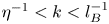 $\eta ^{-1} < k < l_{B}^{-1}$. The present results are consistent with those of Bogucki et al. (Reference Bogucki, Domaradzki and Yeung1997) who observed that the
  $k^{-1}$ spectral range extends to
  $k < \eta ^{-1}$; see also Yeung et al. (Reference Yeung, Xu and Sreenivasan2002) for a similar observation. Antonia & Orlandi (Reference Antonia and Orlandi2002) commented on the possibility that the onset of the VCR occurs when
  $r$ is greater than
  $\eta$. The VCR is followed by a transition range which marks the gradual diminishing effect of
  $\nu$ with increasing
  $r/\eta$ and leading to the ICR. When
  $Pr$ decreases from 1 to
  $10^{-7}$, a range of scales, which is commonly denoted as the inertial–diffusive range, emerges and increases to the detriment of the ICR. Notice that the magnitude of
  $S_{ \phi ^{2}}$ decreases as
  $Pr$ decreases, reflecting an increase of the scalar diffusivity
  $\alpha$, and thus a stronger diffusion of the scalar
  $\phi$. The inset of figure 8 shows the EDQNM calculations of
  $S_{\phi ^{2}}$ in decaying HIT for
  $Re_\lambda =1000$ (
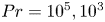 $Pr=10^{5}, 10^{3}$ and 1) and 20 000 (
 $Pr=10^{-3}$ and
  $10^{-5}$) (Briard & Gomez Reference Briard and Gomez2015, Reference Briard and Gomez2016) and HIT in the presence of uniform mean scalar gradient for
 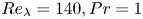 $Re_\lambda =140, Pr = 1$, 32, and 512 (Buaria et al. Reference Buaria, Clay, Sreenivasan and Yeung2021b). We use the EDQNM and DNS spectra (the spectra of Buaria et al. (Reference Buaria, Clay, Sreenivasan and Yeung2021b) are from their supplementary material) to calculate
  $S_{\phi ^{2}}$ according to (5.1). The EDQNM data suggest the emergence of a plateau as
  $Pr$ increases beyond 1 while the inertial–diffusive range increases to the detriment of the ICR as
  $Pr$ decreases below 1. The DNS data also indicate a trend for the emergence of a plateau with increasing
  $Pr$. This trend is less marked than in the EDQNM data perhaps due to the relatively lower value of the Reynolds number.

Figure 8. Effect of  $Pr$ on the distribution of
  $S_{\phi ^{2}}/\overline {\phi ^{2}}$ for
  $Re_\lambda = 1.15 \times 10^{7}$. The different subranges identified at the top refer to
  $Pr=10^{7}$. Inset: EDQNM calculations for
  $Re_\lambda = 1000$ (black line) and
 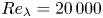 $Re_\lambda = 20\,000$ (red line),
  $Pr=10^{5}, 10^{3}$, 1,
  $10^{-3}$ and
  $10^{-5}$ (Briard & Gomez Reference Briard and Gomez2016). Blue lines: DNS (Buaria et al. Reference Buaria, Clay, Sreenivasan and Yeung2021b),
 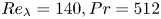 $Re_\lambda =140, Pr= 512$ (dashed line), 32 (dot-dashed line) and 1 (dotted line).
Some comments with regard to the present calculations are warranted. It is quite remarkable that while the model (2.5) does not explicitly account for the effect of  $Pr$ and
  $R$ is kept constant, the calculations do capture the expected effect of an increasing
  $Pr$, that is, the emergence of a VCR observed in the EDQNM data and to some extent in the DNS data. Nevertheless, the present results shown in figure 8, need to be considered with caution. Indeed, it is most likely that
  $R$ will vary with
  $Pr$. One can perhaps expect that the variation of
  $R$ should have an impact on the results if such a variation is explicitly accounted for in the model. For example, the emergence of the plateau in
  $S_{\phi ^{2}}$ could be more gradual and less ‘abrupt’ than for the present prediction and more in line with the trend of the EDQNM and DNS data. A possible first attempt, which is beyond the scope of the present study, to account for the variation of
  $R$ with
  $Pr$ can be carried out using the relation
 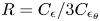 $R= C_\epsilon /3C_{\epsilon _\theta }$, where
  $C_\epsilon$ is approximately constant (
 $\simeq 0.5$) when
  $Re_\lambda \gtrsim 100$ in HIT (Donzis et al. Reference Donzis, Sreenivasan and Yeung2005; Ishihara et al. Reference Ishihara, Gotoh and Kaneda2009). If the dependence of
  $C_{\epsilon _\theta }$ on
  $Pr$ is known, one can obtain the dependence of
  $R$ on
  $Pr$. For example, figure 2 of Buaria et al. (Reference Buaria, Clay, Sreenivasan and Yeung2021a) shows that
  $C_{\epsilon _\theta }$ varies like
  $1/\log Pr$ when
  $Re_\lambda =140$ and
  $Pr$ varies from 1 to 512 leading to
  $R \sim \log Pr$. Finally a few words are warranted regarding the calculations at very large values of
  $Re_\lambda$ (e.g.
  $O(10^{7}))$ and
  $Pr$ (e.g.
  $O(10^{7}))$. For such values of
  $Re_\lambda$, one expects the flow to be hypersonic and is unlikely to be observed in the laboratory or in the atmosphere. The results shown in figures 7 and 8 for very large
  $Re_\lambda$ and
  $Pr$ should be considered qualitative if not speculative.
6. Conclusions
We have solved numerically the linearly forced transport equation (1.1) for  $\overline {( \delta \phi )^{2}}$, the second-order scalar function, using a closure model for
  $-\overline {(\delta u)( \delta \phi )^{2}}$, the third-order mixed velocity–scalar structure function. The closure, which exploits the analogy between the turbulent kinetic energy and passive scalar variance fields when
  $Pr=1$, is based on a gradient-type hypothesis with an eddy-viscosity model proposed by Djenidi & Antonia (Reference Djenidi and Antonia2021) for the third-order velocity structure function
  $\overline {( \delta u)^{3}}$. Further, a linear ‘forcing’ (4.2), similar to that introduced by Lundgren (Reference Lundgren2003) for the transport equation of (
 $\overline {(\delta u)^{2}}$), replaces the integral term in (1.1) in order to mimic steady-state HIT.
The calculated distributions of  $\overline {( \delta \phi )^{2}}$ are tested against data reported in the literature and based on measurements and numerical simulations for
  $Pr= 0.7$ and 1. The agreement between the present calculations and published experimental and numerical data is very good lending confidence to the model (2.5) for closing the transport equation (1.1). However, the agreement deteriorates when
  $Pr$ differs significantly from 1. Yet, the calculations reproduce the effect expected when
  $Pr$ is varied. For example, as
  $Pr$ increases, a range of scales emerges between the viscous–diffusive range and ICR, where
  $\overline {( \delta \phi )^{2}}$ remains constant. This range corresponds to the
  $k^{-1}$ spectral range in the three-dimensional scalar spectrum, but differs from that predicted by Batchelor (Reference Batchelor1959). Also when
  $Pr$ decreases below 1, the calculation captures the expansion of the inertial–diffusive range to the detriment of the ICR.
Acknowledgements
We thank A. Briard for providing us with his EDQNM data. We also thank the reviewers for their constructive comments.
Funding
S.L.T. wishes to acknowledge support given to him from NSFC through grants 11702074 and 91952109 and from the Research Grants Council of Shenzhen Government through grant RCYX20210706092046085.
Declaration of interest
The authors report no conflict of interest.


 Open access