


1. Introduction
The Reynolds analogy is one of the essential building blocks for the theoretical description of the energy equation in wall-bounded flows. It expresses a similarity between momentum exchange and the specific, i.e. temperature-difference-related, heat transfer in certain fluid flows, and hence can be seen as the essential basis of most turbulence models for the energy equation in turbulent flows. For compressible flows, it further forms the basis of most fundamental compressible concepts (for instance, Morkovin's hypothesis), which all rely on arguments based on the Reynolds analogy. For wall-bounded flows, the overall effect of the Reynolds analogy can be determined by considering only the ratio between the specific wall heat flux and the wall shear stress, which is commonly known as the Reynolds analogy factor  $s$ with
 \begin{equation} s\equiv\frac{2c_{h}}{c_{f}}=\frac{\bar{q}_{w}{u}_{e}}{\bar{\tau}_{w}c_{p}\left({T}_{w}-\bar{T}_{r}\right)}.\end{equation}
Here  $c_{f}\equiv \bar {\tau }_{w}/({\rho }_{e}{u}_{e}^{2}/2)$ is the skin-friction coefficient and
  $c_{h}\equiv \bar {q}_{w}/({\rho }_{e}{u}_{e}c_{p}({T}_{w}-\bar {T}_{r}))$ the heat transfer coefficient, i.e. the Stanton number. The subscript
  $e$ indicates flow properties evaluated at the boundary-layer edge
  $y=\delta _e$. Bar denote Reynolds (ensemble) averaged values, while values that do not have a fluctuation component are denoted without bars;
  $\bar {\tau }_w$ is the mean wall shear stress,
  $\bar {q}_{w}$ the wall heat flux in the wall-normal direction
  $y$,
$y$,  ${T}_w$ the prescribed wall temperature,
  $\bar {T}_r$ the adiabatic wall (recovery) temperature and
  $c_p$ the specific heat at constant pressure. The Reynolds analogy factor is an excellent representation of the Reynolds analogy because it reflects the integral effect of the momentum and heat transfer across the boundary layer at the wall.
For turbulent flows, however, the behaviour of the exact Reynolds analogy factor  $s$ (and hence the Reynolds analogy in general) is complex,and observed trends have often not been validated due to the lack of high-quality data. For zero-pressure-gradient (ZPG) conditions, on the one hand,
  $s$ is surprisingly insensitive to variations in
  ${T}_w$ (or
  $\bar {q}_{w}$), Reynolds number or Mach number; see e.g. Duan, Beekman & Martin (Reference Duan, Beekman and Martin2010), Duan & Martin (Reference Duan and Martin2011) and Zhang et al. (Reference Zhang, Bi, Hussain and She2014). On the other hand, influences such as surface roughness (see e.g. Forooghi et al. Reference Forooghi, Weidenlener, Magagnato, Boehm, Kubach, Koch and Frohnapfel2018; Peeters & Sandham Reference Peeters and Sandham2019) and pressure gradients, among others, have strong effects on
  $s$. Under pressure-gradient conditions, the Reynolds analogy factor is influenced by the particular pressure distribution in the streamwise direction, and also variations in
  ${T}_w$ (or
  $\bar {q}_{w}$) have an impact if combined with pressure gradients, as is known for laminar cases; see Cohen & Reshotko (Reference Cohen and Reshotko1955). From the point of view of literature, the quantitative influence of streamwise pressure gradients on
  $s$ is largely unknown, because both measurements and simulations of heat transfer are essentially non-existent, even for situations where the flows are in some state of streamwise self-similarity (except in the work of Houra & Nagano (Reference Houra and Nagano2006) and Araya & Castillo (Reference Araya and Castillo2013)), a state from which the most generic conclusions can be drawn. Note that the term self-similarity only refers to the approximated state of self-similarity for the outer layer and not for the entire boundary layer as a whole; see Gibis et al. (Reference Gibis, Wenzel, Kloker and Rist2019) for a detailed discussion.
1.1. Influence of streamwise pressure gradients
The strong influence of the pressure gradient on the Reynolds analogy factor is made immediately obvious by considering the limiting case of a separating boundary layer. While the skin friction (coefficient) tends to zero ( $c_f \rightarrow 0$) as the velocity gradient at the wall tends to zero, the heat-transfer coefficient
  $c_h$ remains finite since the (specific) heat transfer primarily occurs via conduction at the wall regardless of the pressure gradient, leading to
  $s \rightarrow +\infty$. Hence, by concluding the considerable variation of
  $2c_h/c_f$ results from the fact that
  $c_h$ is much less sensitive to changes in the streamwise pressure gradient than
  $c_f$ in incompressible conditions, it is expected that in comparison to ZPG cases,
  $s$ increases for adverse-pressure-gradient (APG) cases and decreases for favourable-pressure-gradient (FPG) cases; see e.g. Tetervin (Reference Tetervin1969). For self-similar laminar flows, this behaviour is well studied and documented, see Cohen & Reshotko (Reference Cohen and Reshotko1955).
In turbulent boundary layers (TBLs), turbulent mixing is the dominant mechanism for energy and momentum transfer, and convection replaces conduction as the primary heat-transfer process. For boundary layers subjected to pressure gradients, the dominant role of turbulent mixing intuitively should, therefore, make turbulent flows less sensitive to the effect of streamwise pressure gradients compared to laminar ones (Bons Reference Bons2005). For incompressible TBLs the only analytical attempt based on classical self-similarity solutions can be found in the little-known work of So (Reference So1994), where the self-similarity analysis by Mellor & Gibson (Reference Mellor and Gibson1966) for the momentum equation has been extended to the energy equation. The meaningfulness of the analytical results derived has been assessed by Bons (Reference Bons2005) by comparison with experimental data, which, however, cannot reliably be assumed to stem from a well converged near-equilibrium state. Nevertheless, the predicted (or expected) trends of pressure-gradient influences could be at least qualitatively confirmed.
For compressible TBLs in pressure-gradient conditions, it is not obvious to what extent the incompressible trends can be simply transferred. The streamwise evolution of the skin-friction factor  $c_f$ (and hence also
  $c_h$) is difficult to predict even under self-similar conditions, making the behaviour of
  $s$ non-trivial; see Wenzel et al. (Reference Wenzel, Gibis, Kloker and Rist2019). Strictly speaking, the Reynolds analogy is expected to apply to both sub- and supersonic cases; for compressible self-similar laminar flows the influence of Mach number is usually negligible for
  $T_w/T_0=const.$ (see Cohen & Reshotko Reference Cohen and Reshotko1955 for details). It can, therefore, also be expected that for the Reynolds analogy factor
  $s$ in compressible TBLs subjected to pressure gradients no significant Mach-number dependence exists. This is supported by the fact that the adiabatic recovery factor
  $r$, which is closely linked to the Reynolds analogy, is also only slightly influenced in these conditions; see Wenzel et al. (Reference Wenzel, Gibis, Kloker and Rist2019). However, since to our knowledge there is no verified theoretical prediction of
  $s$, the quantitative behaviour of
  $s$ is largely unknown, both in the incompressible and the compressible regime.
1.2. Objectives of this study
Summarizing, the overall effect of pressure gradients on the Reynolds analogy factor  $s$ is far from well described or understood. For non-equilibrium conditions, the boundary layers are somewhat arbitrarily influenced by history effects, making general conclusions very difficult, if not impossible. In Wenzel et al. (Reference Wenzel, Gibis, Kloker and Rist2019) and Gibis et al. (Reference Gibis, Wenzel, Kloker and Rist2019), direct numerical simulation (DNS) data of (approximate) self-similar compressible TBLs have been made available, which are unique both in terms of the length of the self-similar regions and the degree of self-similarity achieved for the outer layer. These data provide the opportunity to describe the effect of pressure gradients on the Reynolds analogy factor
  $s$ with high reliability for the first time. By dealing with both sub- and supersonic data, it is further possible to estimate Mach number effects on
  $s$. By only considering near-adiabatic wall conditions, a first step towards a systematic description of the pressure-gradient behaviour of
  $s$ in both compressible and incompressible TBLs is presented. Two main questions are addressed: how is the Reynolds analogy factor
  $s=2c_h/c_f$ influenced by non-zero pressure-gradient conditions, and does the Mach number play a role? The present study is structured as follows. All DNS conducted are briefly summarized in § 2. The main part, the pressure-gradient dependence of the Reynolds analogy factor
  $s$, is discussed in § 3, and concluding remarks are given in § 4.
2. Simulation details
This study is based on DNS results for self-similar compressible TBLs with pressure gradients presented in Wenzel et al. (Reference Wenzel, Gibis, Kloker and Rist2019) for inflow Mach numbers of  $M_{\infty ,0}=0.5$ and
  $M_{\infty ,0}=2.0$. To allow for a meaningful determination of
  $c_h$, the relevant cases have been recomputed with near-adiabatic fixed wall temperatures. For the subsonic cases, the wall temperature
  ${T}_w$ is set to be
  ${+}10\ \textrm {K}$ above the adiabatic one taken from the fully adiabatic reference cases in Wenzel et al. (Reference Wenzel, Gibis, Kloker and Rist2019), yielding
  ${T}_w/\bar {T}_r\approx 1.03$. For the supersonic cases, the wall temperature is set to be
  $+20K$ above the adiabatic references, yielding
  ${T}_w/\bar {T}_r\approx 1.04$. Note that the recovery temperature is a function of
  $x$ with pressure gradient, and so is the prescribed wall temperature. To ensure that the wall heating does not noticeably affect the results in comparison to fully adiabatic conditions, the strongest subsonic APG case
  $iAPG_{\beta _K=1.05}$ also has been recomputed with a wall temperature of
  $-10\ \textrm {K}$ below the adiabatic one; all results shown in the following have been found to be almost unaffected and thus can be considered almost adiabatic. Determined with the incompressible form of the displacement thickness
  $\delta ^*_K=\int _0^{\delta _{99}}( 1-\bar {u}/u_e )\,\textrm {d}y$ as a length scale,
  $\beta _K=(\delta ^*_K/\bar {\tau }_w)(\textrm {d}p_e/\textrm {d}x)$ denotes the kinematic Rotta–Clauser parameter, which allows a comparison of pressure-gradient influences between compressible and incompressible cases; see Wenzel et al. (Reference Wenzel, Gibis, Kloker and Rist2019) and Gibis et al. (Reference Gibis, Wenzel, Kloker and Rist2019). Boundary-layer-edge values (index
  $e$) are determined at the wall-normal position where the spanwise vorticity
  $\omega _z$ drops below
  $10^{-6}$ of its wall value, similarly to Spalart & Strelets (Reference Spalart and Strelets2000). Evaluated at the beginning and the end of the self-similar regions, relevant boundary-layer properties are summarized in table 1 for all cases. Given parameters are the Mach number at the boundary-layer edge
  $M_e$, the Reynolds numbers
  $Re_\tau =\bar {\rho }_w u_\tau \delta _{99}/{\mu }_w$,
  $Re_{\delta ^*_K}=\rho _e u_e \delta ^*_K/\mu _e$,
  $Re_{\delta ^*_{K,w}}=\rho _w u_e \delta ^*/\mu _w$ and the resulting wall-to-edge temperature ratios. The displacement and momentum thicknesses used are
  $\delta ^*=\int _0^{\delta _{99}}( 1-( \bar {\rho }\,\bar {u})/(\rho _e u_e ) )\,\textrm {d}y$ and
  $\theta = \int _0^{\delta _{99}} ( \bar {\rho }\,\bar {u})/(\rho _e u_e ) ( 1- \bar {u}/u_e )\,{\textrm {d}y}$, respectively. Details about the spatial extent of the computational domains are identical to the fully adiabatic cases (see Wenzel et al. Reference Wenzel, Gibis, Kloker and Rist2019) and are therefore not repeated. The same holds for the numerical method.
Table 1. Summary of boundary-layer parameters for DNS data. All data are evaluated at the beginning and the end of the self-similar regions. Given parameters are the boundary-layer-edge Mach number  $M_e$, the Reynolds numbers
  $Re_\tau =\bar {\rho }_w u_\tau \delta _{99}/\bar {\mu }_w$,
  $Re_{\delta ^*}=\rho _e u_e \delta ^* / \mu _e$,
  $Re_{\delta _{K,w}^*}=\bar {\rho }_w u_e \delta _{K}^* / \mu _w$ and the wall-to-edge temperature ratio
  $T_w/T_e$; for
  $T_w/\bar {T}_r$ see the text.

2.1. Simulation parameters
In contrast to the fully adiabatic DNS results presented in Wenzel et al. (Reference Wenzel, Gibis, Kloker and Rist2019), the temperature at the solid wall is fixed according to a prescribed temperature distribution  ${T}_w={T}_w(x)$, which hence suppresses any temperature fluctuations at the wall. The pressure is calculated by
  $(\textrm {d}p/{\textrm {d}y})_w=0$. Apart from the change in the wall-temperature boundary condition, the numerical set-up of the supersonic adiabatic cases and the present supersonic cases are identical and therefore not reconsidered here; see Wenzel et al. (Reference Wenzel, Gibis, Kloker and Rist2019) for details. The same applies to the subsonic cases, for which, however, the domain size has been halved in the spanwise direction to reduce the computational costs. A comparison with a reference case computed from the original domain size has shown only negligible effects on the boundary-layer properties discussed in this paper. As for the adiabatic set-ups, the reference thermodynamic flow properties are the inflow far-field temperature
  $T_{\infty ,0}=288.15$ K, inflow far-field density
  $\rho _{\infty ,0}=1.225\ \textrm {kg}\ \textrm {m}^{-3}$, Prandtl number
  $Pr=0.71$, specific gas constant
  $R=287\ \textrm {J}\ \textrm {kg}^{-1}\ \textrm {K}^{-1}$ and ratio of specific heats
  $\gamma =1.4$; these are set equal for all cases. Data averaging is performed over both time and spanwise direction and does not start before the flow has passed the whole domain at least twice. Consistently for all cases and in accordance with the fully adiabatic cases, time averages were computed over a flow-through time corresponding to at least
  $250$ local boundary-layer thicknesses
  $\delta _{99}$ (
 ${\rm \Delta} t u_e/\delta _{99}=250$, where
  ${\rm \Delta} t$ is the averaging period), which corresponds to at least eight eddy-turnover times
  ${\rm \Delta} tu_\tau /\delta _{99}$ for the most restricting APG cases. Both the appropriate convergence of the statistics and the initial transients have been assessed as described in Wenzel et al. (Reference Wenzel, Gibis, Kloker and Rist2019) and Wenzel et al. (Reference Wenzel, Selent, Kloker and Rist2018); see also Bobke et al. (Reference Bobke, Vinuesa, Örlü and Schlatter2017).
3. Reynolds analogy factor
In this section, the streamwise evolution of both  $c_f$ and
  $c_h$ is investigated, before the pressure-gradient dependence of the Reynolds analogy factor
  $s=2c_h/c_f$ is discussed. Special attention needs to be given to the calculation of the (adiabatic) recovery temperature
  $\bar {T}_{r}$ which is chosen to normalize the wall heat flux in the calculation of
  $c_h=\bar {q}_{y,w}/({\rho }_e{u}_ec_p({T}_w-\bar {T}_r))$. To ensure consistent and meaningful results, all
  $\bar {T}_r$-distributions have been taken from the fully adiabatic reference cases.
3.1. Streamwise evolution of  $c_f$ and $c_h$


The streamwise evolution of both  $c_f$ and
  $c_h$ is depicted in figures 1(a) and 1(c) for the sub- and supersonic cases, respectively. For the ZPG cases in both regimes, a grey dotted best-fit curve is plotted approximating
  $c_f$ with
  $c_f=26.515\,Re_\tau ^{-0.318}$ for the subsonic case in panel (a) and
  $c_f=19.896\,Re_\tau ^{-0.335}$ for the supersonic case in panel (c). In comparison to the fully adiabatic cases,
  $c_f$-values are slightly decreased by about
  $1\,\%$ due to the effect of wall-heating. By fitting
  $s$ to match the
  $c_h$-distributions for the ZPG cases, the approximations for
  $c_h$ are calculated from the respective
  $c_f$ by
  $c_h=s(c_f/2)$;
  $s=1.18$ for the subsonic and
  $s=1.16$ for the supersonic cases. To allow for a quantitative evaluation of pressure-gradient influences, all distributions are normalized by the best-fit
  $c_f$-curve of the corresponding ZPG case at the same inlet Mach number in panels (b) and (d). Only regions of approximate self-similarity are depicted.

Figure 1. Streamwise evolution of  $c_f$ and
  $c_h$ for the sub- and supersonic cases in panels (a) and (c), respectively, and normalized with the best-fit for
  $c_f$ of the corresponding ZPG case at same inlet Mach number in panels (b) and (d). For the sub- and supersonic ZPG cases, the best-fits are
  $c_f=26.515\,Re_\tau ^{-0.318}$ and
  $c_f=19.896\,Re_\tau ^{-0.335}$, respectively. The best-fits for
  $c_h$ are computed from
  $c_h=s(c_f/2)$ with calibrated values of
  $s=1.18$ for the subsonic and
  $s=1.16$ for the supersonic case.
First, the subsonic cases of panels (a) and (b) are discussed. As shown in Wenzel et al. (Reference Wenzel, Gibis, Kloker and Rist2019), the  $c_f$-distributions of the subsonic APG cases in panel (a) can be interpreted as a scaling of the ZPG-case distribution. Hence, by scaling with the best-fit curve of the ZPG case, all distributions depicted in panel (b) become constants; the same holds for
  $c_h$. All results show the expected trends introduced in § 1.1. The
  $c_f$-distributions are more influenced by pressure gradients than the
  $c_h$-distributions:
  $c_f$ is decreased by approximately
  $22\,\%$ for the strongest APG case, while
  $c_h$ is increased by only about
  $8\,\%$; compare the
  $y$-axis on the right-hand side of (b).
For the supersonic cases in panels (c) and (d), the  $c_f$-distributions are more complex since pressure-gradient effects and the effect of the varying Mach number in the streamwise direction interact. While the effect of an APG decreases
  $c_f$, the countereffect of decreasing local Mach number increases
  $c_f$; see Wenzel et al. (Reference Wenzel, Gibis, Kloker and Rist2019). In line with the subsonic cases, the
  $c_h$-distributions of the supersonic cases also follow the trends of the
  $c_f$-distributions. However, because of the strong influence of the varying Mach number in the streamwise direction, both
  $c_f$ and
  $c_h$ are increased in the supersonic APG case and decreased in the supersonic FPG case. For the APG case,
  $c_f$ is increased by a maximum of up to
  $10\,\%$, while
  $c_h$ is increased by a maximum of up to
  $45\,\%$. Consequently, in contrast to the incompressible point of view which holds for the subsonic cases (see § 1.1), it cannot be argued for the supersonic cases that the effect of pressure gradients on
  $s$ can be mainly attributed to influences on
  $c_f$, while
  $c_h$ remains almost unchanged.
3.2. Pressure-gradient dependence of the Reynolds analogy factor
The resulting Reynolds analogy factors  $s=2c_h/c_f$ are depicted in figure 2(a) and normalized with the respective ZPG-value at corresponding inflow Mach number
  $s/s_{ZPG}=(2c_h/c_f)/(2c_{h}/c_{f})_{ZPG}$ in (b). All data are plotted versus the kinematic Rotta–Clauser parameter
  $\beta _K$. Cases with
  $\beta _K=0$ are ZPG cases, those with positive
  $\beta _K$ are APG cases and those with negative
  $\beta _K$ are FPG cases. The
  $s$-values are plotted as dots with transparent colour for every 10th data point in the streamwise direction in regions of approximate self-similarity: blue for the subsonic and red for the supersonic cases. Regions near the inlet of the computational domain, where the streamwise pressure gradient is slowly imposed and the resulting flows are not yet self-similar, are depicted as thick, transparently coloured lines for each case. The only analytical attempt based on classical, incompressible self-similarity solutions known to the authors (So Reference So1994) is plotted according to
 \begin{equation} \frac{2c_h}{c_f}=\frac{\kappa^{-1} \ln{\left(Re_{\delta_{K,w}^*}\right)}+B+A\left(\beta_K\right)}{\kappa_\theta^{-1} \ln{\left(Re_{\delta_{K,w}^*}\right)}+B_\theta+A_\theta\left(\beta_K, Pr_t\right)}.\end{equation}
The numerator represents a skin-friction relation for  $2/c_f$ derived by Mellor & Gibson (Reference Mellor and Gibson1966), the denominator a Stanton-number relation for
  $1/c_h$ derived by So (Reference So1994). Both relations are based on overlap arguments between the logarithmic law of the wall and a defect law, where
  $\kappa =0.41$,
  $\kappa _\theta =0.41/Pr_t$ and
  $B=4.9$,
  $B_\theta =3.8$ have been used as the constants of the respective logarithmic law. The respective wake deficit is quantified by
  $A(\beta _K)$ and
  $A_\theta (\beta _K,Pr_t)$ and is obtained from the solutions of the differential equations for the wall-normal velocity and temperature profiles. Note that (3.1) is only valid for small
  $\beta _K$-values up to around
  $\beta _K = {O}(1)$. For higher
  $\beta _K$, where
  $c_f$ tends towards zero, a high-
 $\beta _K$ version has to be used; see Mellor & Gibson (Reference Mellor and Gibson1966) and So (Reference So1994) for details.
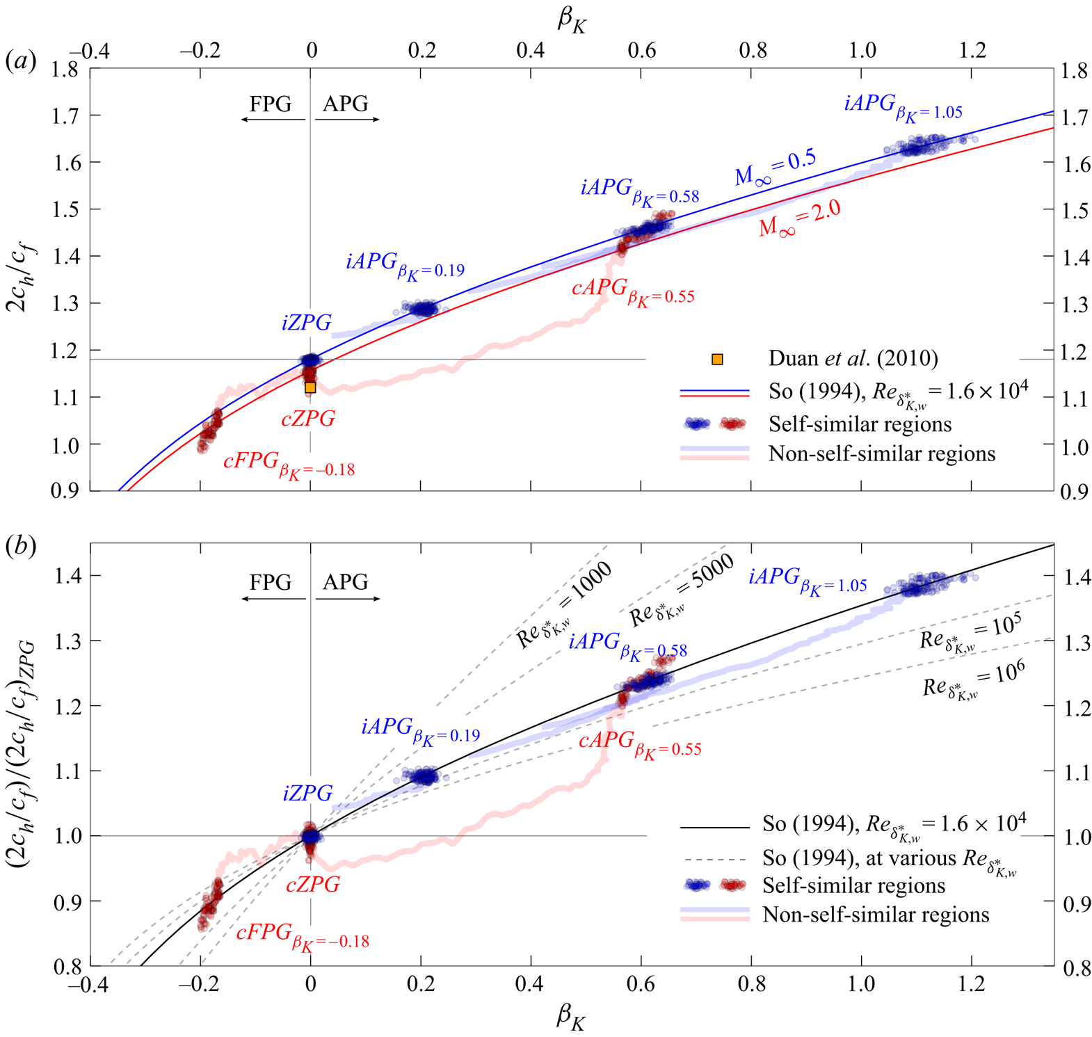
Figure 2. Reynolds analogy factors  $2c_h/c_f$ in (a), normalized with the respective ZPG-value at corresponding Mach number in (b), both plotted as functions of the kinematic Rotta–Clauser parameter
  $\beta _{K}$. Blue and red dots represent results for the sub- and supersonic cases, respectively, evaluated at every 10th data point in the streamwise direction. The analytical reference is computed from (3.1), and the orange square denotes DNS results for a cooled ZPG case from Duan et al. (Reference Duan, Beekman and Martin2010) at
  $M_\infty =5.0$ with
  $T_w/\bar {T}_\delta =3.74$ and
  $T_w/\bar {T}_r=0.68$.
Some comments regarding (3.1) should be made. (i) Some assumptions leading to the general form of the  $c_f$- and
  $c_h$-correlations made by Mellor & Gibson (Reference Mellor and Gibson1966) and So (Reference So1994) are quite restrictive. For example, the von Kármán constant
  $\kappa$ is assumed to be independent of the pressure-gradient parameter
  $\beta _K$, but recent studies suggest a noticeable pressure-gradient dependence; see Vinuesa et al. (Reference Vinuesa, Örlü, Vila, Ianiro, Discetti and Schlatter2017). Nevertheless, the chosen form provides a reasonable starting point for a meaningful estimate. (ii) In the incompressible study by So (Reference So1994), the Reynolds number chosen is the incompressible displacement-thickness Reynolds number
  $Re_{\delta ^*_{inc}}=\rho u_e \delta ^*/\mu$. For compressible data there are multiple choices, two of which are summarized in table 1:
  $Re_{\delta ^*}=\rho _e u_e \delta ^*/\mu _e$ is the compressible defined displacement-thickness Reynolds number, and
  $Re_{\delta _{K,w}^*}=\bar {\rho }_w u_e\delta ^*_K/\mu _w$ is the Reynolds number defined with the kinematic displacement thickness
  $\delta ^*_K$ similar to the Rotta–Clauser parameter
  $\beta _K$. For the present data,
  $Re_{\delta _{K,w}^*}$ is in a comparable range for both the sub- and supersonic cases; see table 1. The influence of the chosen Reynolds number will be further discussed in § 3.2.1. (iii) The next comment refers to the determination of
  $A_\theta (\beta _K,Pr_t)$. Since
  $A_\theta (\beta _K,Pr_t)$ is based on the solution of the differential equation of the temperature profile, it is influenced by the assumptions made in its derivation. This includes in particular the assumption of an eddy viscosity, a constant turbulent Prandtl number and an assumed Reynolds analogy of the form
  $2c_h/c_f=C(\beta _K,Pr_t)$. Because no reference data exist for self-similar pressure-gradient cases with heat transfer, there is almost no quantitative validation of its distribution. (iv) As already shown in So (Reference So1994), the choice of
  $Pr_t$ has a crucial influence on the absolute values of
  $2c_h/c_f$ depicted in figure 2(a), but only a negligible influence on the course of
  $[(2c_h/c_f)/(2c_{h}/c_{f})_{ZPG}]_{So}$ in figure 2(b) if normalized with the ZPG-value. Hence, for practical use, the reference curves in panel (a) are obtained by scaling the normalized reference curve in panel (b) with the DNS value for the ZPG cases of the respective inflow Mach number
  $[(2c_{h}/c_{f})_{ZPG}]_{DNS}[(2c_h/c_f)/(2c_{h}/c_{f})_{ZPG}]_{So}$. Since the choice of
  $Pr_t$ only negligibly influences the results,
  $Pr_t=1.0$ has been chosen in the following for the reference curves, to be consistent with So (Reference So1994).
3.2.1. Self-similar regions
First, the subsonic DNS results, indicated by blue dots, and the blue solid line for the analytically derived relation in figure 2(a) are discussed. Compared to the  $iZPG$ case at
  $\beta _K=0$ with
  $s=2c_h/c_f\approx 1.18$, the Reynolds analogy factor
  $s$ is significantly larger for the subsonic
  $iAPG$ cases with increasing APG strength (blue dots at positive
  $\beta _K$). For the strongest
  $iAPG_{\beta _K=1.05}$ case with
  $\beta _K=1.05$,
  $s$ is approximately
  $40\,\%$ larger than in the
  $iZPG$ case. This is particularly noteworthy since APGs of
  $\beta _K\approx 1$ are only considered to be moderate in the literature. For the subsonic data in the range
  $1000 \lesssim Re_{\delta ^*_{K,w}} \lesssim 5000$ (see table 1), the coloured dots are clustered for each case, implying nearly no Reynolds-number dependency of
  $s$ for the moderate Reynolds-number range considered. This behaviour is in accordance with the intuitive expectation that self-similar solutions imply a state of
  $s$ in which there is only a low dependence on the Reynolds number. In contrast to the DNS data, the analytical relation by So (Reference So1994) (see (3.1)) exhibits a high Reynolds-number sensitivity. If determined for the Reynolds numbers obtained from the DNS, a streamwise variation of
  $s$ by about
  $25\,\%$ is suggested for
  $1000\lesssim Re_{\delta ^*_{K,w}}\lesssim 5000$; compare the reference curves for
  $Re_{\delta ^*_{K,w}}=1000$ and
  $Re_{\delta ^*_{K,w}}=5000$ in panel (b). It is worth mentioning, however, that So's correlation (like most self-similarity analysis for turbulent flows) is applicable to high-Reynolds-number flows only in a strict sense. Nevertheless, the pressure-gradient influences on
  $s$ observed in the DNS are perfectly predicted by the reference with an empirically calibrated, virtual Reynolds number of
  $Re_{\delta _{K,w}^*}=16\,000$ (with
  $Pr_t=1.0$). Therefore, it can be concluded that
  $A_\theta (\beta _K,Pr_t)$, which is the only parameter influenced by
  $\beta _K$ in the denominator, nearly perfectly reflects pressure-gradient influences on
  $c_h$ and thus on
  $s$. The role of
  $Re_{\delta _{K,w}^*}$, in contrast, might be much more limited to a constant, which, once calibrated, appears to be valid for a large Reynolds-number range. The possibility cannot be excluded, however, that for sufficiently high Reynolds numbers a clear Reynolds-number trend will be observed. According to So, this trend would tend towards lower
  $s$-values.
A comparison between the subsonic and the supersonic ZPG cases shows a slight Mach-number influence; compare the blue and red dots at  $\beta _K=0$. For the supersonic
  $cZPG$ case,
  $s=2c_h/c_f\approx 1.16$, which is approximately
  $2\,\%$ smaller than for the subsonic case. An orange symbol is added which represents the temporal DNS result by Duan et al. (Reference Duan, Beekman and Martin2010) for a moderately cooled TBL at
  $M=5.0$ to allow for an estimate for higher Mach numbers. It should be recalled that no clear influence of the wall temperature has been found in the literature, which hence should make the reference comparable to the present near-adiabatic cases. The reference data support the Mach-number trend observed; however, differences caused by different set-ups or by variations in computing the adiabatic reference temperature cannot be reliably assessed.
A comparison between the subsonic  $iAPG_{\beta _K=0.58}$ case and the supersonic
  $cAPG_{\beta _K=0.55}$ case shows very good agreement; compare the blue and red dots at
  $\beta _K\approx 0.6$. If at all, the
  $s$-values of the supersonic case are slightly below those of the subsonic case, which could confirm the slight Mach-number influence observed for the ZPG cases also for the APG regime. The only minor influence of the local Mach number in pressure-gradient conditions is in accordance with laminar investigations, where
  $s$ is mostly assumed not to be influenced by the local Mach number
  $M_e$; see e.g. Cohen & Reshotko (Reference Cohen and Reshotko1955). Combining the only minor influence of the Mach number on
  $s$ with the assumption that the Mach-number influence is comparable in the ZPG and pressure-gradient cases, the subsonic analytical reference curve has been scaled to fit the supersonic ZPG case at
  $\beta _K=0$; this is depicted as a solid red line. For the supersonic
  $cFPG_{\beta _K=-0.18}$ with
  $\beta _K=-0.18$, the red reference and the DNS data are in good agreement.
To eliminate the Mach-number effects observed, the results of figure 2(a) are repeated in figure 2(b), but normalized with the respective  $s$-value for a corresponding ZPG case at the same Mach number. To correctly incorporate Mach-number effects in pressure-gradient conditions, all results at every streamwise position have to be scaled by their own ZPG reference at a corresponding Mach number in a strict sense. To roughly account for the effect of Mach number, results for the
  $cAPG_{\beta _K=0.55}$ case with local Mach numbers between
  $M_e=1.77$ and
  $M_e=1.4$ have been scaled with a reference slightly below the compressible
  $cZPG$ case (
 $s=1.17$), and those for the
  $cFPG_{\beta _K=-0.18}$ case (
 $M_e$ up to
  $2.36$) with a reference slightly above the compressible ZPG case (
 $s=1.185$).
3.2.2. Non-self-similar behaviour
All results discussed so far are only valid for near-adiabatic pressure-gradient cases with a very high degree of self-similarity of the outer layer in the streamwise direction; only these regions of the DNS computed have been evaluated so far. Since all computations start from ZPG conditions at the inflow of the domain, all cases also include non-self-similar regions where the pressure gradient is applied, but the self-similarity is not yet established. These regions are characterized by a non-constant Rotta–Clauser parameter  $\beta _K$, implying that the streamwise evolution of the outer layer cannot be represented by only a simple set of characteristic scales; see Gibis et al. (Reference Gibis, Wenzel, Kloker and Rist2019). These regions are depicted as transparently coloured thick lines in figure 2. Based on these results, the universality of the conclusions previously drawn from the self-similar regions can be assessed for non-self-similar regions.
For the subsonic cases, the thick blue lines in figure 2(b) closely follow the black reference curve for the self-similar results. Both  $c_f$ and
  $c_h$ hence rapidly and synchronously react to the streamwise pressure variation without being too strongly influenced by the non-self-similar history of the analysed boundary layers. Consequently, (3.1) allows for a very good approximation of local
  $s$-values for non-self-similar nearly incompressible TBLs as well, if the local
  $\beta _K$-values are known. For fully adiabatic flows where
  $c_h$ is not defined, this further allows for a rough estimation of local
  $c_h$-values.
For the supersonic cases, the  $s$-values show large deviations from the analytical reference in regions of non-self-similarity. For the APG case, the corresponding
  $s$-values are significantly too low, and for the FPG case slightly too large, in comparison to those of self-similar flows. In contrast to the subsonic cases, local values of the Reynolds analogy factor
  $s$, therefore, do not depend only on the local
  $\beta _K$-value, but also on the global pressure distribution, or in other words, the upstream history of the boundary layer.
4. Conclusions
A quantitative study of  $c_f$,
  $c_h$ and the related Reynolds analogy factor
  $s=2c_h/c_f$ for self-similar sub- and supersonic turbulent boundary layers with pressure gradients in the streamwise direction has been conducted up to moderate Reynolds numbers. For the subsonic, nearly incompressible cases, the
  $c_f$- and
  $c_h$-distributions show the expected results, i.e.
  $c_f$ is much more strongly affected by pressure gradients than
  $c_h$. For the supersonic cases, pressure-gradient influences are complex and affect both
  $c_f$ and
  $c_h$; in our cases
  $c_h$ is more influenced. Computed from the respective
  $c_f$- and
  $c_h$-distributions, the resulting Reynolds analogy factor is greatly increased for adverse-pressure-gradient conditions and decreased for favourable-pressure-gradient conditions. For the strongest subsonic adverse-pressure-gradient case with
  $\beta _K=1.05$,
  $s$ is increased by about
  $40\,\%$ in comparison to zero-pressure-gradient conditions. A comparison between sub- and supersonic cases shows only a small Mach-number influence, which is in a comparable range for zero-pressure-gradient and pressure-gradient cases;
  $s$ is slightly lower for the supersonic cases. Although the DNS cover quite a large Reynolds-number range from small to moderate Reynolds numbers, no Reynolds-number dependency is found for
  $s$ in the parameter range investigated. This is remarkable since Reynolds-number effects should be noticeable if present, especially for low Reynolds numbers, where high-Reynolds-number assumptions are questionable. The variation of
  $s$ with pressure-gradient parameter
  $\beta _K$ is found to agree with the analytical relation by So (Reference So1994) if calibrated to fit the DNS data. However, this only holds if a fixed, virtual Reynolds number is assumed for calibration. For the non-self-similar conditions occurring in the upstream region of the domain of interest,
  $s$ is found to follow closely the self-similar trends for the subsonic cases. For the supersonic adverse-pressure-gradient case, however, the corresponding
  $s$-values are significantly lower, and for the favourable-pressure-gradient case higher, in comparison to the self-similar state.
Acknowledgements
The financial support of the Deutsche Forschungsgemeinschaft (DFG), under reference numbers RI680/38-1 and WE6803/1-1, and the provision of computational resources on Cray XC40 and NEC SX-Aurora TSUBASA by the Federal High-Performance Computing Center, Stuttgart (HLRS), under grant GCS Lamt (LAMTUR), ID 44026, are gratefully acknowledged.
Declaration of interests
The authors report no conflict of interest.


 Open access