


1. Introduction
Purely elastic instabilities, i.e. those in which the Reynolds number ( $Re$) is vanishingly small and inertia can play no role, in viscoelastic flows occur frequently due to the nonlinear nature of the elastic stresses generated not only in simple viscometric flows but also in more complex flows with so-called ‘mixed’ kinematics of shear and extension. Generally, beyond a critical value of the Weissenberg number (
 $Wi$) – the ratio of elastic to viscous stresses – the ‘simple’ solution branch of the base state (i.e. steady and/or symmetric) in such flows bifurcates to a more complex flow either spatially or temporally. A geometry that allows the study of mixed kinematics but where elongational flow is important is the so-called ‘cross-slot’ geometry, which is used frequently in extensional-flow related studies (Haward et al. Reference Haward, Oliveira, Alves and McKinley2012b). This geometry consists of four bisecting rectangular channels with two sets of opposing inlets and outlets. These opposing inlets and outlets produce a flow field with a free-stagnation point. At this point the velocity is zero and a finite velocity gradient in the streamwise direction appears. In principle, due to the zero velocity at this point, a fluid element is trapped for an ‘infinite’ time, generating a significant strain and potentially enabling ‘steady-state’ extensional-flow kinematics to be realized. Such an effect is a hallmark of this geometry and the reason it is often proposed as an extensional rheometer (Haward et al. Reference Haward, Oliveira, Alves and McKinley2012b). Gardner et al. (Reference Gardner, Pike, Miles, Keller and Tanaka1982) were the first to report a steady asymmetric flow field for viscoelastic fluids in this geometry, although the much later study carried out by Arratia et al. (Reference Arratia, Thomas, Diorio and Gollub2006) was the first in which this phenomenon was suitably characterized and such an asymmetric distribution of the flow field was unequivocally associated with a purely elastic instability. Interestingly, this instability has been reproduced numerically by Poole, Alves & Oliveira (Reference Poole, Alves and Oliveira2007) using the upper convected Maxwell (UCM) model, which is an unsatisfactory model for any steady-state extensional flow beyond a critical strain rate, and finite extensible nonlinear elastic (FENE)-type models by Rocha et al. (Reference Rocha, Poole, Alves and Oliveira2009). Since then, there have been a number of experimental and numerical studies on the effects of various parameters on the onset and development of the elastic instabilities in cross-slot flows (Haward et al. Reference Haward, Ober, Oliveira, Alves and McKinley2012a; Sousa et al. Reference Sousa, Pinho, Oliveira and Alves2015; Cruz et al. Reference Cruz, Poole, Afonso, Pinho, Oliveira and Alves2016; Haward, McKinley & Shen Reference Haward, McKinley and Shen2016; Kalb, Villasmil-Urdaneta & Cromer Reference Kalb, Villasmil-Urdaneta and Cromer2018; Sousa, Pinho & Alves Reference Sousa, Pinho and Alves2018). However, so far, there is no prediction of the corresponding instability beyond the bifurcation point using linear stability for two-dimensional purely elongational flows (Lagnado & Leal Reference Lagnado and Leal1990; Wilson Reference Wilson2012). One should note that, in this geometry, although a nominally purely elongational flow is observed at the stagnation point, due to the existence of re-entrant corners (Dean & Montagnon Reference Dean and Montagnon1949; Moffatt Reference Moffatt1964; Davies & Devlin Reference Davies and Devlin1993; Hinch Reference Hinch1993), a fluid particle may experience a complex mix of shear and extensional deformation as it flows through the domain. Recently, Davoodi, Domingues & Poole (Reference Davoodi, Domingues and Poole2019) suggested the use of a cylinder at the geometric centre of the cross-slot geometry to investigate the effect on the onset of instability. This geometric modification applies a fundamental difference on the flow field as the finite value of the strain rate at the free-stagnation point in the standard geometry is replaced with zero-strain-rate pinned stagnation points at the surface of the cylinder. The resulting data showed that the suggested modification, although significantly changing the flow distribution in the region near the stagnation point, does not change the nature of the symmetry-breaking instability or, for small cylinders, the critical condition for onset. It was therefore concluded that the instability cannot be solely related to the extensional flow near the stagnation point but it is more likely related to streamline curvature and the high deformation rates towards the corners i.e. a classic ‘curved streamlines’ purely elastic instability (Shaqfeh Reference Shaqfeh1996). In Davoodi et al. (Reference Davoodi, Domingues and Poole2019), using a combination of an analytical approach and supporting numerical simulations, it was shown that, by controlling the size of the cylinder, and consequently the curvature of streamlines, one may be able to control/delay onset of the instability to higher
  $Wi$. A well-known dimensionless parameter which rationalizes these types of ‘curved streamline’ instabilities is the
  $M$ parameter introduced by McKinley, Pakdel & Öztekin (Reference McKinley, Pakdel and Öztekin1996) (often referred to as the ‘Pakdel–McKinley’ criterion) which is defined as
 \begin{equation} M=\sqrt{\frac{\tilde{\lambda} \tilde{U}}{\tilde{\mathcal{R}}}\frac{\tilde{\tau}_{11}}{\tilde{\eta}_0 \tilde{\dot{\gamma}}}}, \end{equation}
where  $\tilde{U}$ is a reference velocity,
  $\tilde{\lambda}$ is the relaxation time,
  $\tilde{\mathcal{R}}$ is the curvature of the streamline,
  $\tilde {\tau }_{11}$ is the elastic normal stress in the streamwise direction,
  $\tilde {\eta }_0$ is the zero-shear-rate viscosity of the fluid and
  $\tilde {\dot {\gamma }}$ is the magnitude of the shear rate. This parameter can be considered as the viscoelastic complement of the Görtler number (Görtler Reference Görtler1955). In (1.1), the first term on the right-hand side shows the ratio of a characteristic length
  $\tilde {\lambda }\tilde {U}$ over which disturbance information is convected before it decays to the streamline curvature (this term can also be referred to as a local Deborah number, showing the ratio of the relaxation time of the fluid to the time a disturbance takes to travel along a streamline). The second term on the right-hand side of (1.1) is added to scale properly the effect of the normal stress in the streamwise direction with a reference stress scale. This term is generally of the same order of magnitude as a local Weissenberg number, which is the destabilizing term in the disturbance equation (McKinley et al. Reference McKinley, Pakdel and Öztekin1996). Equation (1.1) proposes that the kinematic and dynamic conditions corresponding to the curvature of the flow and the tensile elastic stress along the streamlines, respectively, can be combined into a single dimensionless criterion that must be exceeded for the onset of purely elastic instabilities. Using this approach, Haward et al. (Reference Haward, McKinley and Shen2016) have shown that in an ideal planar elongational flow, such as that observed in the optimized-shape cross-slot extensional rheometer, the purely elastic instability may also be triggered due to strong streamline curvature close to the stagnation point.
In two-phase flow problems, the influence of the capillary number ( $Ca$) on the interface shape, and so on the streamline curvature, of two fluids has been studied in many different problems (e.g. Chinyoka et al. Reference Chinyoka, Renardy, Renardy and Khismatullin2005; Capobianchi et al. Reference Capobianchi, Pinho, Lappa and Oliveira2019; Zografos et al. Reference Zografos, Afonso, Poole and Oliveira2020). In such situations, across the interface of two fluids, a jump in normal forces is balanced by the curvature of the interface and the interfacial tension. As an example, in studies related to drop motion and deformation, Taylor & Acrivos (Reference Taylor and Acrivos1964) have shown that by increasing
  $Re$ the shape of Newtonian droplets may change from a spherical shape to an oblate shape, which is related to the nonlinear contribution of the inertial force. Such complex deformations are attributed to the presence of a non-uniform distribution of the normal forces at the interface of two fluids. Due to this non-uniform jump of the normal stress, at a constant interfacial tension, a non-uniform distribution of curvature is required to balance the applied forces (so the droplet loses its constant-curvature spherical shape). In such problems, it is well known that, by increasing the interfacial tension, one can change this distribution of the curvature along the interface of two fluids to retain the spherical shape of the droplet. The use of the interfacial tension as an important parameter in the evolution of a disturbance at the interface of two fluids has been studied in many different two-phase flow instabilities (see for example Graham Reference Graham2003; Lee, Kim & Kim Reference Lee, Kim and Kim2011).
For viscoelastic fluids, all previous studies in the cross-slot were restricted to a single fluid phase. In this work, a series of two-phase flow simulations were performed, supported by Newtonian experiments, and some limited three-dimensional (3-D) calculations, to investigate the effect of different viscoelasticities in each inlet arm, viscosity jumps across the interface and the interfacial tension applied at the boundary of two different fluids injected from opposing inlets of the cross-slot geometry. By increasing the interfacial tension to a sufficiently large value, one may hope to influence the streamline curvature  $\tilde{\mathcal{R}}$ in the central region of the cross-slot geometry. Thus we postulate that the interfacial tension may be used as a means to control the symmetry-breaking instability.
2. Geometric and problem set-up configuration
Here, we consider two-phase flows through cross-slot geometries. A schematic of the problem being studied is presented in figure 1. In this study, inlets are located at the left (fluid-1) and right (fluid-2) side arms while outlets are located at the top and bottom arms. The width  $\tilde {W}$ of all inlet and outlet arms are the same. We consider both 2-D and 3-D configurations with different aspect ratios
  $\varLambda ={\tilde {H}}/{\tilde {W}}$, where
  $\tilde {H}$ is the depth of the channel, which is considered constant throughout. Two different fluids are injected at the inlets with an equal constant bulk velocity
  $\tilde {U}_B$. We consider a range of fluid pairs, both miscible and immiscible (referred to throughout as two ‘phases’ for simplicity) to study the effect of viscosity ratio,
  $K={\tilde {\eta }_{2,t}}/{\tilde {\eta }_{1,t}}$ with
  ${\tilde {\eta }_{1,t}}$ and
  ${\tilde {\eta }_{2,t}}$ being the total viscosity of fluid-1 and fluid-2, and capillary number,
  $Ca$ on the interface and on the onset of elastic instabilities. We combine 2-D and 3-D numerical simulations together with analytical solutions and experiments in microfluidic devices to characterize the flow field for both Newtonian and viscoelastic fluid flows.

Figure 1. (a) Schematic of the cross-slot geometry with insets highlighting the notation used in 3-D (top right) and a typical 2-D computational mesh (bottom left). Here,  $\tilde {h}$ indicates the passage width of fluid-1 in the outlet arms. (b) Schematic illustrating the experimental microfluidic cross-slot apparatus allowing for direct observation of the
  $(x, y)$ plane. Not to scale.
3. Governing equations and numerical method
Numerical approaches to simulate a two-phase flow field may be divided into two main categories, known as ‘interface-tracking’ and ‘interface-capturing’ methods. Amongst the interface-tracking methods, such as immersed boundary (Peskin Reference Peskin1982; Mittal & Iaccarino Reference Mittal and Iaccarino2005), front-tracking (Tryggvason et al. Reference Tryggvason, Bunner, Esmaeeli, Juric, Al-Rawahi, Tauber, Han, Nas and Jan2001) and boundary integral (Peterlin Reference Peterlin1976) methods have received considerable attention due to their accurate prediction of the shape of the interface at the boundary of the two fluids. In such methods, a moving sharp boundary is considered to track the interface of the two fluids. Tracking methods are known to be accurate for most flows but due to singularity issues in problems with morphological change, such as the ones observed in droplet breakup and coalescence (Jacqmin Reference Jacqmin1999; Yue et al. Reference Yue, Feng, Liu and Shen2004; Magaletti et al. Reference Magaletti, Picano, Chinappi, Marino and Casciola2013), cannot be used for these types of simulations. Also, due to the presence of a moving mesh (which needs to be updated and reconstructed in every time step in the simulation), such methods are expensive with respect to their simulation computational time.
In contrast, in numerical simulations involving interface-capturing methods, the mesh could be either static (i.e. fixed grid distribution) or dynamic and the interface between two fluids is defined based on the variation of a scalar phase indicator parameter  $\tilde {C}$. The volume of fluid (VOF) and phase-field (PF) methods are arguably the most popular interface-capturing methods (Hirt & Nichols Reference Hirt and Nichols1981). For VOF and PF, this scalar quantity is usually related to a volume fraction or a mass concentration. In these methods, the scalar parameter
  $\tilde {C}$ varies in between two limits (mostly
  $0 \leq \tilde {C} \leq 1$), with
  $\tilde {C}$ equal to the lower and upper limits being indicative of fluid-1/fluid-2, respectively. The interface of the two fluids is specified where
  $\tilde {C}$ exhibits a mid-value in between these two limits (in the current case
  $\tilde {C}=0.5$). In the VOF method, in order to find the evolution of
  $\tilde {C}$, generally, the classic transport diffusion equation is solved, while in the PF model, this equation has an additional double-well potential term in comparison with the classic diffusion equation. In these methods, the system is dealt with as one single fluid with variable properties. By solving the transport equation for
  $\tilde {C}$, one can define different properties in space and time based on the regions that different fluids flow and treat the interfacial tension as a body force.
In the current work, the VOF method is used to find the variation of the  $\tilde {C}$ parameter in both space and time domains, the standard advection transport equation using a velocity field
  $\boldsymbol {\tilde {u}}$ is solved as
 \begin{equation} \frac{\partial \tilde{C}}{\partial \tilde{t}}+ \boldsymbol{\tilde{u}}\boldsymbol{\widetilde{\nabla}} \tilde{C}=0, \quad 0\leq \tilde{C} \leq 1. \end{equation}
For a binary fluid composed of fluid-1 and fluid-2, once the space/time distribution of  $\tilde {C}$ is known, one can define the following equations as was recommended in the viscoelastic toolbox RheoTool version 4.1 (Pimenta & Alves Reference Pimenta and Alves2017):
 \begin{gather} \tilde{\rho}= \tilde{C} \tilde{\rho}_1+(1-\tilde{C}) \tilde{\rho}_2, \end{gather}
 \begin{gather} \tilde{\eta}_s= \tilde{C} \tilde{\eta}_{s,1}+(1-\tilde{C}) \tilde{\eta}_{s,2}, \end{gather}
 \begin{gather} \boldsymbol{\tilde{\tau}}= \tilde{C} \boldsymbol{\tilde{\tau}_{1}}+(1-\tilde{C}) \boldsymbol{\tilde{\tau}_{2}}, \end{gather}
where indices 1 and 2 indicate fluid-1 and fluid-2,  $\widetilde {\eta _s}$ is the solvent viscosity,
  $\tilde {\rho }$ is the density and
  $\boldsymbol {\tilde {\tau }}$ is the viscoelastic contribution of the stress tensor. The governing equations for the motion of this fluid are conservation of mass, assuming incompressibility, and momentum
 \begin{gather} \boldsymbol{\widetilde{\nabla}} \boldsymbol{\cdot} \boldsymbol{\tilde{u}}=0, \end{gather}
 \begin{gather} \tilde{\rho} \left(\frac{\partial \boldsymbol{\tilde{u}}}{\partial \tilde{t}} +\boldsymbol{\tilde{u}}\boldsymbol{\cdot}\boldsymbol{\widetilde{\nabla}} \boldsymbol{\tilde{u}}\right) ={-}\boldsymbol{\widetilde{\nabla}} \tilde{p} +\boldsymbol{\widetilde{\nabla}} \boldsymbol{\cdot}\boldsymbol{\tilde{\tau}}+\boldsymbol{\widetilde{\nabla}}\boldsymbol{\cdot} \left(\tilde{\eta}_{s} \left(\boldsymbol{\widetilde{\nabla}}\boldsymbol{\tilde{u}}+\boldsymbol{\widetilde{\nabla}}\boldsymbol{\tilde{u}}^\textrm{T}\right)\right) +\boldsymbol{\tilde{F}}, \end{gather}
where  $\tilde {p}$ is the pressure and
  $\boldsymbol {\tilde {F}}$ is the capillary force applied at the interface of the two fluids due to the existence of the interfacial tension and is calculated as follows (Figueiredo et al. Reference Figueiredo, Oishi, Afonso, Tasso and Cuminato2016; Brackbill, Kothe & Zemach Reference Brackbill, Kothe and Zemach1992):
 \begin{equation} \boldsymbol{\tilde{F}}=\tilde{\sigma} \tilde{\kappa} \boldsymbol{{n}} \tilde{\delta}_i=\tilde{\sigma} \tilde{\kappa}\boldsymbol{\widetilde{\nabla}}\tilde{C}, \end{equation}
where  $\tilde {\sigma }$ is the surface tension coefficient,
  $\tilde {\kappa }=-\boldsymbol {\widetilde {\nabla }}\boldsymbol {\cdot } \boldsymbol {n}$ is the interface curvature,
  $\boldsymbol {n}={\boldsymbol {\widetilde {\nabla }}\tilde {C}}/{\|\boldsymbol {\widetilde {\nabla }}\tilde {C}\|}$ is the unit vector normal to the interface (Francois et al. Reference Francois, Cummins, Dendy, Kothe, Sicilian and Williams2006) and
  $\tilde {\delta }_i$ is the
  $\delta$-function at the interface. Here, to simulate the viscoelastic contribution of the stress tensor (i.e.
  $\tilde {\boldsymbol {\tau }}$), the simplified Phan-Thien and Tanner (sPTT) constitutive equation is employed which is derived from network theory (Phan-Thien & Tanner Reference Phan-Thien and Tanner1977) and is a suitable model for simulation of shear-thinning polymeric fluids (Bird, Armstrong & Hassager Reference Bird, Armstrong and Hassager1987). The extra-stress tensor using the sPTT model may be calculated as follows:
 \begin{equation} f_i\boldsymbol{\tilde{\tau}_i}+\tilde{\lambda}_i \stackrel{\boldsymbol{\widetilde{\nabla}}}{\boldsymbol{\tilde{\tau}_i}}=\tilde{\eta}_{p,i}(\boldsymbol{\nabla} \boldsymbol{\tilde{u}}+\boldsymbol{\nabla} \boldsymbol{\tilde{u}}^\textrm{T}) \quad i=\{1,2\}, \end{equation}
where index  $i$ can be either 1 or 2 (i.e.
  $i=\{1,2\}$) indicating fluid-1 and fluid-2. Here, the
  $f_i$ function for the linear-sPTT model is defined as
 \begin{equation} f_i=1+\alpha_i \frac{\tilde{\lambda}_i}{\tilde{\eta}_{p,i}}Tr(\boldsymbol{\tilde{\tau}_i}) \quad i=\{1,2\}, \end{equation}
where  $\alpha$ is the extensibility parameter. In the limiting case of
  $\alpha =0$ the sPTT constitutive equation reduces to the Oldroyd-B model and if additionally
  $\tilde {\eta }_s=0$, the UCM model is recovered. The upper-convective derivative of the extra-stress tensor,
  $\stackrel {\boldsymbol {\widetilde {\nabla }}}{\boldsymbol {\tilde {\tau }}_i}$, is defined as
 \begin{equation} \stackrel{\boldsymbol{\widetilde{\nabla}}}{\boldsymbol{\tilde{\tau}}_i}= \frac{\textrm{D}}{\textrm{D}\tilde{t}}(\boldsymbol{\tilde{\tau}}_i) -\left(\boldsymbol{\tilde{\tau}_i}\boldsymbol{\cdot}\boldsymbol{\widetilde{\nabla}} \boldsymbol{\tilde{u}}+\boldsymbol{\widetilde{\nabla}} \boldsymbol{\tilde{u}}^\textrm{T}\boldsymbol{\cdot}\boldsymbol{\tilde{\tau}_i}\right)\quad i=\{1,2\}, \end{equation}
where the material derivative of an arbitrary matrix  $\boldsymbol {A}$ is defined as
  $({\textrm {D}}/{\textrm {D}\tilde {t}})(\boldsymbol {A})=({\partial \boldsymbol {A}}/{\partial \tilde {t}}+ \boldsymbol {\tilde {u}}\boldsymbol {\cdot }\boldsymbol {\widetilde {\nabla }} \boldsymbol {A})$. To solve the series of equations presented in (3.1)–(3.10) the rheoInterFoam solver in the rheoTool package of OpenFoam is used (Pimenta & Alves Reference Pimenta and Alves2017).
A zero gradient boundary condition for the stress and velocity components is applied at the outlets to simulate fully developed conditions. At the walls, values of the stress components are calculated using an extrapolation method, as suggested by Pimenta & Alves (Reference Pimenta and Alves2017) and no slip is assumed for the velocities. For the phase indicator parameter  $\tilde {C}$, constant values of 1 and 0 are used at the left and right inlet arms and a zero gradient at the outlet and walls (cf. figure 1). The flow domain has been divided into 5 smaller sub-domain blocks (four inlet/outlet arms and one central block). Most simulations were carried out using a mesh similar in density to that of Cruz et al. (Reference Cruz, Poole, Afonso, Pinho, Oliveira and Alves2016) (table 1). Additionally, some limited 3-D simulations are also carried out to study the effect of the
  $K$ parameter and
  $Ca$ on the interface shape and location. The effect of mesh refinement on the numerical simulations is presented in table 2 and figure 8 for 2-D and 3-D cases, respectively. In table 2, the effect on the critical Weissenberg number for two different uniform meshes are shown for different capillary numbers. The total number of cells for the M21 and M22 meshes are 13 005 and 51 005, respectively and the error between these two calculated critical Weissenberg numbers are less than
  $1\,\%$. Similar to this, two different meshes, consisting of 663 255 and 5 151 505 cells, have been used to study the effect of mesh on the ‘dimple size’ – discussed later in § 7 – of 3-D geometries and the error was calculated to also be smaller than
  $1\,\%$. These results give us sufficient confidence to continue our study with the smaller of the meshes in both 2-D and 3-D cases.
Table 1. Characteristics of the computational meshes. NC is number of cells,  $\tilde {W}$ is channel width and
  $\tilde {H}$ is channel height.

Table 2. Mesh dependency study for 2-D simulations using mesh M21 with 13 005 and mesh M22 with 51 005 cells.

4. Non-dimensionalization
In our analysis, to better characterize the flow field and the important parameters playing a role in this problem, the following dimensionless parameters are adopted:
 \begin{align} \left. \begin{gathered} x=\frac{\tilde{x}}{\tilde{W}}, y=\frac{\tilde{y}}{\tilde{W}}, z=\frac{\tilde{z}}{\tilde{W}}, \varLambda=\frac{\tilde{H}}{\tilde{W}}, \boldsymbol{U}=\frac{\tilde{\boldsymbol{u}}}{\tilde{U}_B}, \boldsymbol{\tau}=\frac{\tilde{ \boldsymbol{\tau}}}{\tilde{\eta}_{1,t}\tilde{U}_B/\tilde{W}}, p=\frac{\tilde{p}}{\tilde{\eta}_{1,t}\tilde{U}_B/\tilde{W}},\\ Re_i=\frac{\tilde{\rho}_i \tilde{U}_B \tilde{W}}{\tilde{\eta}_{i,t}},Wi_i=\frac{\tilde{\lambda}_i \tilde{U}_B}{\tilde{W}}, \beta_i=\frac{\tilde{\eta}_{i,s}}{\tilde{\eta}_{i,t}}, Ca=\frac{\tilde{\eta}_{1,t} \tilde{U}_B}{\tilde{\sigma}}, K=\frac{\tilde{\eta}_{2,t}}{\tilde{\eta}_{1,t}}, AP=\frac{\tilde{Q}_{i1}-\tilde{Q}_{i2}}{\widetilde{Q_i}}, \end{gathered} \right\} \end{align}
where index  $i$ can be either 1 or 2 (i.e.
  $i=\{1,2\}$) indicating properties of fluid-1 and fluid-2,
  $\tilde {x}$,
  $\tilde {y}, \tilde {z}$ are the variables related to the Cartesian coordinate system,
  $\tilde {W}$ is the width and
  $\tilde {H}$ is the depth of the channel,
  $\varLambda$ is the cross-section aspect ratio,
  $\tilde {\boldsymbol {u}}$ is the velocity vector,
  $\tilde {U}_B$ is the imposed bulk velocity at the inlets,
  $\tilde {\boldsymbol {\tau }}$ is the extra-stress tensor,
  $\tilde {p}$ is the pressure,
  $Re_i$ is the Reynolds number in each inlet stream and was set to be
  $10^{-3}$ for all simulations in order to model creeping flow,
  $Wi_i$ is the Weissenberg number defined for each phase,
  $\beta _i$ is the solvent-to-total viscosity ratio of each of the two phases and
  $\tilde {\eta }_{i,t}$ is the total viscosity of each of the phases (i.e.
  $\tilde {\eta }_{i,t}=\tilde {\eta }_{i,s}+\tilde {\eta }_{i,p}$),
  $Ca$ is the capillary number defined based on the properties of fluid-1,
  $K$ is the ratio of total viscosity of fluid-2 to fluid-1 (and so
  $CaK$ is the capillary number based on fluid-2),
  $\widetilde {Q_i}$ is the imposed flow rate at the inlets (i.e. in the two-dimensional problem
  $\widetilde {Q_i}=\tilde {W}\tilde {U}_B$),
  $\tilde {Q}_{i1}$ and
  $\tilde {Q}_{i2}$ are defined in figure 1 and
  $AP$ is the asymmetry parameter used in our simulations to quantify the magnitude of asymmetry in the flow (before onset of any symmetry-breaking instability
  $\tilde {Q}_{i1}=\tilde {Q}_{i2}$ so
  $AP=0$, but once the symmetry of the flow is broken
  $\tilde {Q}_{i1}\neq \tilde {Q}_{i2}$ and
  $AP$ exhibits a non-zero value). A previous study conducted by Wilson & Rallison (Reference Wilson and Rallison1997) has shown that a non-zero value of the normal-stress jump at the interface of viscoelastic fluids may trigger an instability in three-layer planar flows. In this work, to concentrate on two key effects we study the effect of either varying the elasticity of each fluid stream (but in the limit of negligible interfacial tension) or keeping the elasticity fixed, but interfacial tension can be varied. The values of
  $\beta _1=\beta _2=1/9$ and the extensibility parameter of two fluids
  $\alpha _1=\alpha _2=0.02$ are held fixed to reduce the parameter space.
5. Experimental
Experiments in 3-D microfluidic planar channels were carried out to visualize the Newtonian flow field for comparison with the numerical results and to study the effect of aspect ratio. A schematic diagram of the experimental rig is shown in figure 1. The experimental microchannels were made from polydimethylsiloxane (Sylgard 184, Dow Corning) and were fabricated using a SU-8 mould by standard soft-lithography techniques. Three different cross-slot microfluidic devices with varying aspect ratios ( $\varLambda = \tilde {H}/\tilde {W}$) were used:
  $\varLambda =0.83, \varLambda =0.28$ and
  $\varLambda =0.22$. To study the effect of viscosity ratio, deionized water and a variety of gycerol/water solutions were prepared with viscosities ranging from 6.47 mPa s to 300 mPa s (cf. table 3). In addition, for the experiments on the effect of interfacial tension, perfluorodecalin (Sigma Aldrich,
  $\tilde {\eta } = 6.7$ mPa s) was used together with the most viscous gycerol/water solution tested (
 $\tilde {\eta } = 300$ mPa s). The interfacial tension between these two fluids was measured to be
  $35.03 \pm 0.04$ mN m
 $^{-1}$ at 293.2 K. The fluids were characterized in steady shear on a DHR-2 hybrid rotational rheometer (TA Instruments) with a cone-plate geometry (60 mm diameter,
  $1^{\circ }$ cone angle) at a temperature of 293.2 K. The surface tension and interfacial tension measurements were carried out with a drop shape analyser (model DSA25, Kruss) using the pendant-drop method, in which the shape of the pendant drop was fit using the Young–Laplace equation
 \begin{equation} \Delta \tilde{p}= \tilde{\sigma}\left(\frac{1}{\tilde{r}_1}+\frac{1}{\tilde{r}_2}\right), \end{equation}
where  $\Delta \tilde {p}$ is the pressure difference across the interface and
  $\tilde {r}_1$ and
  $\tilde {r}_2$ are the principal radii of curvature of the interface. A high-precision syringe pump with independent modules (neMESYS, Cetoni GmbH) was used for precise fluid control, imposing flow rates in the range
  $\tilde {Q} \leq 2.5\ \textrm {ml}\ \textrm {h}^{-1}$, yielding a maximum Reynolds number
  $Re \leq 3.0$ (based on the less viscous fluid properties as reference). SGETM gastight syringes of appropriate volumes were used to ensure that the syringe pump pulsation-free minimum dosing rate is exceeded. The flow was illuminated with a 100 W metal halide lamp and visualized using an inverted microscope (Olympus IX71), equipped with a 20X objective lens, a CCD camera (Olympus XM10) and an adequate filter cube (Olympus U-MWIGA3). For flow visualization rhodamine-B (Sigma-Aldrich) was added to one of the inlet streams. In addition, a number of experiments were also carried out using streak photography in which the fluids were seeded with
  $1\ \mathrm {\mu }\textrm {m}$ fluorescent tracer particles (FluoSpheres carboxylate-modified, Nile Red (Ex/Em: 535/575 nm)) at concentration of approximatly
  $0.02\,\%wt$. Long exposure photography was used to capture the flow patterns at the centre plane of the microchannel (
 $\tilde {z} = \tilde {H}/2$).
Table 3. Characterization of different fluids used in the experiment.

 $^*$Reference fluid for all cases is water, except for the 91.8 wt
 $\%$ glycerol and water solution, for which the viscosity ratio is reported relative to HPF10.
6. Analytical solutions for two-phase flow of fully developed Newtonian fluids in a channel and rectangular ducts
It is well known that in the limit of no inertia or surface tension, channel flows of Newtonian fluids with a viscosity stratification are potentially linearly unstable (Yih Reference Yih1967), nevertheless, in this section, exact analytical solutions for the pressure driven, creeping two-phase fully developed flow of Newtonian fluids in a 1-D channel between two infinite parallel plates (figure 2a) and rectangular cross-sections (figure 2b) are derived. These solutions will then provide a partial benchmark solution for the nonlinear simulations in the cross-slot geometry (i.e. in the outlet arms sufficiently far downstream of the cross-slot where the flow becomes ‘fully developed’). To avoid Yih-type instability, the numerical simulations include interfacial tension (Hooper & Boyd Reference Hooper and Boyd1983; Barmak et al. Reference Barmak, Gelfgat, Vitoshkin, Ullmann and Brauner2016). A schematic of the problem and the employed coordinate system is shown in figure 2. In the limit of no inertia, or fully developed flow, the Navier–Stokes equation in dimensionless form for fluid-1 and fluid-2 can be written as
 \begin{gather} \nabla^2 U_i=G, \quad i=1 \end{gather}
 \begin{gather} K\nabla^2 U_i=G, \quad i=2 , \end{gather}
where  $U_i$ is the dimensionless velocity in the
  $\tilde {y}$ direction with respect to the reference bulk velocity (i.e.
  $U_i={\tilde {U}_i}/{\tilde {U}_B}$) and
  $G$ is the dimensionless pressure gradient defined as
  $G={({\partial \tilde {p}}/{\partial \tilde {y}})}/{({\tilde {\eta }_1\tilde {U}_B}/{\tilde {W}^2})}$. Note that, to obtain a rectilinear 1-D flow distribution, the pressure drop in both phases must be equal, otherwise it will lead to a pressure gradient in the lateral direction of the flow resulting in a secondary motion. Solutions to (6.1)–(6.2) for 1-D channel flows may be presented as follows:
 \begin{gather} U_{1,2D}=\tfrac{1}{2}Gx_1^2+C_1x_1+C_2, \end{gather}
 \begin{gather} U_{2,2D}=\tfrac{1}{2}\frac{G}{K}x_1^2+C_3x_1+C_4, \end{gather}
and similarly for rectangular 2-D ducts as
 \begin{gather} U_{1,2D}=\sum_{n=1}^{n=\infty}\left(A_1cosh\left( \frac{n{\rm \pi} x_1}{\varLambda} \right) +A_2sinh\left(\frac{n{\rm \pi} x_1}{\varLambda} x\right) +\frac{2G(1-({-}1)^n)}{n^3{\rm \pi}^3}\right)sin(n{\rm \pi} z_1), \end{gather}
 \begin{gather} U_{2,2D}=\sum_{n=1}^{n=\infty}\left(A_3cosh\left( \frac{n{\rm \pi} x_1}{\varLambda} \right) +A_4sinh\left( \frac{n{\rm \pi} x}{\varLambda} x_1\right)+\frac{2G(1-({-}1)^n)}{K n^3{\rm \pi}^3}\right)sin(n{\rm \pi} z_1), \end{gather}
where  $x_1$ and
  $z_1$ are the dimensionless variables in the rectangular coordinate system (i.e.
  $x={\tilde {x}}/{\tilde {W}}$ and
  $z={\tilde {z}}/{\varLambda \tilde {W}}$). Equations (6.3)– (6.6) should be solved subject to continuity of tangential velocity and shear stress at the interface i.e.
  $x=\tilde {h}/\tilde {w}=h$ as
 \begin{gather} U_1|_{x_1=h}=U_2|_{x_1=h}, \end{gather}
 \begin{gather} \frac{\textrm{d} U_1}{\textrm{d} x_1}|_{x_1=h}=K\frac{\textrm{d} U_2}{\textrm{d} x_1}|_{x_1=h}, \end{gather}
and the no-slip boundary condition at the walls. For 1-D channel flows, solving these equations with respect to the previously mentioned boundary condition leads to
 \begin{equation} \left. \begin{gathered} C_1=C_3=\frac{3(Kh^2-h^2+1)}{h^2(Kh^2-h^2-2h+3)},\\ C_2=0, C_4={-}\frac{3(Kh-k-h+1)}{h^2(Kh^2-h^2-2h+3)}, \end{gathered} \right\} \end{equation}
and for 2-D rectangular channels, assuming a flat interface (i.e.  $Ca=0$), leads to
 $$\begin{gather} A_1=2({-}1 + ({-}1)^n)\left(cosh\left(\frac{1}{\varLambda} n{\rm \pi}\right)(K - 1)cosh \left(\frac{1}{\varLambda} n {\rm \pi}\right)^2 \right.\nonumber\\ -\, (K - 1)\left(sinh\left(\frac{1}{\varLambda} n {\rm \pi}h\right)sinh\left(\frac{1}{\varLambda} n {\rm \pi}\right) \right.\nonumber\\ \left.\left.+\, cosh\left(\frac{1}{\varLambda} n {\rm \pi}\right)\right) cosh\left(\frac{1}{\varLambda} n {\rm \pi}h\right) + sinh\left(\frac{1}{\varLambda} n {\rm \pi}\right) (K - 1)sinh\left(\frac{1}{\varLambda} n {\rm \pi}h\right)\right.\nonumber\\ \left.\left. +\, cosh\left(\frac{1}{\varLambda} n {\rm \pi}\right) - 1\right) G\right/\left({\rm \pi}^3 \left(sinh\left(\frac{1}{\varLambda} n {\rm \pi}\right)(K - 1) cosh\left(\frac{1}{\varLambda} n {\rm \pi}h\right)^2\right.\right.\nonumber\\ \left.\left. - \,sinh\left(\frac{1}{\varLambda} n {\rm \pi}h\right) cosh\left(\frac{1}{\varLambda} n {\rm \pi}\right)(K - 1) cosh\left(\frac{1}{\varLambda} n {\rm \pi}h\right) - K sinh\left(\frac{1}{\varLambda} n {\rm \pi}\right)\right) n^3\right), \end{gather}$$
 $$\begin{gather} A_2=2G({-}1 + ({-}1)^n)/(n^3{\rm \pi}^3), \end{gather}$$
 $$\begin{gather} A_3=2 \left((K - 1) cosh\left(\frac{1}{\varLambda} n {\rm \pi}h\right)^2 - cosh\left(\frac{1}{\varLambda} n {\rm \pi}\right) (K - 1) cosh\left(\frac{1}{\varLambda} n {\rm \pi}h\right)\right.\nonumber\\ \left.+ \,K \left(cosh(\frac{1}{\varLambda} n {\rm \pi}) - 1\right)\right) ({-}1 + ({-}1)^n)\nonumber\\ G\left/\left({\rm \pi}^3 \left(sinh\left(\frac{1}{\varLambda} n {\rm \pi}\right) (K - 1) cosh\left(\frac{1}{\varLambda} n {\rm \pi}h\right)^2 \right.\right.\right.\nonumber\\ \left.\left.- \,sinh\left(\frac{1}{\varLambda} n {\rm \pi}h\right) cosh\left(\frac{1}{\varLambda} n {\rm \pi}\right) (K - 1) cosh\left(\frac{1}{\varLambda} n {\rm \pi}h\right)- K sinh\left(\frac{1}{\varLambda} n {\rm \pi}\right)\right) n^3 K\right), \end{gather}$$
 $$\begin{gather} A_4={-}2 ({-}1 + ({-}1)^n) \left((K - 1) \left(sinh\left(\frac{1}{\varLambda} n {\rm \pi}h\right) - sinh\left(\frac{1}{\varLambda} n {\rm \pi}\right)\right) cosh\left(\frac{1}{\varLambda} n {\rm \pi}h\right) \right.\nonumber\\ \left.\left. + \,K sinh\left(\frac{1}{\varLambda} n {\rm \pi}\right)\right) G\right/\left({\rm \pi}^3 \left(sinh\left(\frac{1}{\varLambda} n {\rm \pi}\right) (K - 1) cosh\left(\frac{1}{\varLambda} n {\rm \pi}h\right)^2 \right.\right.\nonumber\\ \left.\left.-\, sinh\left(\frac{1}{\varLambda} n {\rm \pi}h\right) cosh\left(\frac{1}{\varLambda} n {\rm \pi}\right) (K - 1) cosh\left(\frac{1}{\varLambda} n {\rm \pi}h\right)\right.\right.\nonumber\\ \left.\left.-\, K sinh\left(\frac{1}{\varLambda} n {\rm \pi}\right)\right) n^3 K\right). \end{gather}$$
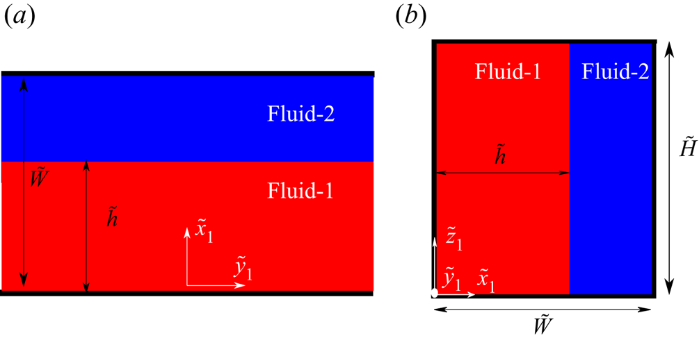
Figure 2. Schematic of (a) the 1-D channel geometry (flow is left to right) and (b) the 2-D rectangular duct geometry (flow is into page) and the employed coordinate system. Not to scale. Note choice of coordinate system to match that of ‘outlet’ arms in cross-slot.
One should note that, along with the unknown constants ( $C_1-C_4$ and
  $A_1-A_4$ in 1-D and 2-D problems, respectively), values of
  $G$ and
  $h$ are also unknown but they can be calculated by setting the flow rate of each fluid to be equal. In the 1-D problem we consider the flow rate in each phase to be equal to
  $\tilde {U}_B\tilde {W}/2$ (or in our dimensionless form equal to 0.5). Using the flow rate constraint for fluid-1, one can calculate the unknown pressure gradient
  $G$ for the 1-D problem as
 \begin{equation} G={-}\frac{6(Kh-h+1)}{h^2(Kh^2-h^2-2h+3)}, \end{equation}
which is equal in both fluids. Setting the flow rate to the value of 0.5 for fluid-2, leads to the following constraint for the variable  $h$
$h$
 \begin{equation} \frac{0.5+(0.5-0.5K^2)h^4+(4K-2)h^3+(3-6K)h^2+(2K-2)h}{h^2K(3+(K-1)h^2-2h)}=0. \end{equation}
For the 1-D problem, the unknown value of  $h$ can be obtained, now, by solving (6.15) numerically. In this work, a bisection method has been used to solve this (Chapra & Canale Reference Chapra and Canale2010). A similar approach can be used to calculate the unknown values of
  $G$ and
  $h$ in the 2-D problem, which, due to the series form of the problem and large size of the equations, are not presented here.
7. Results and discussion
In this section, results obtained using the analytical solutions, numerical simulations and some supporting experiments for two-phase flows of both Newtonian and viscoelastic fluids in the cross-slot geometry are presented.
7.1. Newtonian fluids
To better understand the effect of the various parameters playing a role in this problem, a discussion on the location and shape of the interface of two Newtonian fluids in the fully developed section of the outlet arms is first carried out. This discussion will then be used to qualitatively investigate the effect of these parameters on the important kinematics of the flow field near the corners of the cross-slot geometry, which are known to be regions driving the instability for the viscoelastic case (Davoodi et al. Reference Davoodi, Domingues and Poole2019). Similar to the idea used by Davoodi et al. (Reference Davoodi, Lerouge, Norouzi and Poole2018) for normalization of the aspect ratio, here, a modified form of the viscosity ratio parameter is defined as
 \begin{equation} K^*=\frac{K}{K+1}. \end{equation}
Using this definition, when the viscosity ratio  $K$ changes from zero to infinity, the modified form of the viscosity ratio
  $K^*$ varies from zero to one, respectively. For the 1-D problem, using (6.15), one can say that, by changing the viscosity ratio parameter, the term
  $h(1-h)$ should show two roots at
  $K^*=0$ and
  $K^*=1$. So, in the limits of
  $K \rightarrow 0$ and
  $K \rightarrow \infty$, the
  $h$ parameter tends toward one and zero, respectively. Similarly, for
  $K=1$ (
 $K^*=0.5$) (i.e. fluids in each phase have identical properties), one can easily show analytically that
  $h=0.5$.
Knowing that experiments are necessarily carried out in finite cross-section aspect ratio domains, in figure 3 we analyse the variation of the position of the boundary between the two fluids, represented here via use of  $h(1-h)$ plotted against the normalized viscosity ratio parameter
  $K^*$ using both 2-D and 3-D numerical solutions for four different aspect ratios (the corresponding analytical solutions are simply one-dimensional and two-dimensional as there is no variation in the flow direction due to the fully developed assumption). The analytical results are shown to be in good agreement with the experimental and numerical results. Note that at
  $Ca=\infty$, i.e. when interfacial tension is zero, due to the jump of normal forces at the interface the flow may be unstable (Yih Reference Yih1967) and one might need to use large interfacial tension to avoid such instability (Hooper & Boyd Reference Hooper and Boyd1983; Barmak et al. Reference Barmak, Gelfgat, Vitoshkin, Ullmann and Brauner2016). Considering the fact that it is impossible to obtain
  $Ca=0$, i.e. interfacial tension equal to infinity, the numerical results for
  $0< K^*<0.5$ presented in figure 3 were carried out at a high value of the interfacial tension (
 $Ca=0.005$) and the
  $h(1-h)$ parameter is calculated downstream of the central cross such that the flow is fully developed. A series of complimentary simulations with
  $Ca=\infty$ were also carried out for
  $0.5< K^*<1$. As was also previously reported initially by Yih (Reference Yih1967), our numerical simulations suggest that, in the absence of interfacial tension, the flow may be unstable and the interface in the neutral direction is no longer flat (figure 4). In these cases, the value of
  $h$ obtained numerically and experimentally is taken at the central plane
  $z=0.5$. Knowing that this instability is observed due to the nonlinear nature of the convection terms in the Navier–Stokes equation, one may expect that, by reducing the Reynolds number, the size of the disturbance along the interface should reduce and eventually, at
  $Re=0$, the flow, and consequently the interface of the two fluids, should obtain a steady-state form. Interestingly, in both the numerical simulations and experimental procedure, the location of the interface of the two fluids is shown to be quasi-static, in agreement with the results of Bonhomme et al. (Reference Bonhomme, Morozov, Leng and Colin2011) using similar systems (water and glycerol solutions), which is related to the very small value of the Reynolds number (
 $Re \approx 10^{-3}$) in these cases (Yih Reference Yih1967). Thus, it should be recognized that, outside of our 2-D simulations, the experiments and numerical simulations (with high
  $Ca$) may not be truly steady state, although, as the interface remains essentially constant in time, we will treat them as so. For all aspect ratios, the effect of the normalized viscosity ratio parameter is exactly symmetric about
  $K^*=0.5$ (i.e.
  $K=1$), highlighting the inherent symmetry in the problem. From the results presented in figure 3, it is clear that by increasing the viscosity of one of the two fluids, considering that the pressure drop should be equal in both phases, to retain a rectilinear flow, the average velocity of the more viscous fluid reduces, and so the area required to satisfy the constant flow rate constraint increases. Our analytical and experimental results suggest that this effect is magnified as the aspect ratio is reduced.

Figure 3. Variation of the height of the interface between two fluids with viscosity ratio for Newtonian fluids. The values of the numerical simulations presented in the ranges  $0< K^*<0.5$ and
  $0.5< K^*<1$ are taken in the outlet arms for
  $y=5\tilde {W}$ with
  $Ca=0.005$ and
  $Ca=\infty$, respectively.

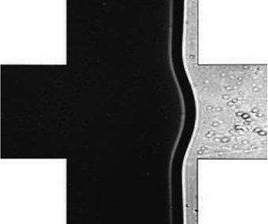
Figure 4. Visualization of the interface between two Newtonian fluids in the fully developed region of the outlet arm with  $Ca\rightarrow \infty$ and viscosity ratios (a)
  $K=1$, (b)
  $K=0.16$, (c)
  $K=0.03$ (where the fluid shown in dark grey is the most viscous one) using
  $\varLambda =0.83$ (i) in the experiment and (ii–iii) in numerical simulations. Figures (i) and (ii) are presented in
  $(x, y)$ plane centred at
  $z=0$ for
  $1.5< y<2$ while (iii) show a cross-sectional view of the channel (
 $(x,z)$ plane) at
  $y=1$.
Figure 4(i) shows the interface of two fluids in the fully developed region of the outlet arm ( $1< y<1.4$) observed in our experiments. As also shown in figure 3, if the viscosity of the two fluids is identical (i.e.
  $K=1$ or
  $K^*=0.5$), the interface is located at the mid-distance between the two walls, as the
  $K$ parameter exhibits a non-unity value the more viscous fluid moves the interface such that the average velocity decreases in this phase and increases for the less viscous phase. By changing
  $K$, one can clearly see the appearance of a ‘shadow’ region at the interface. The presence of this shadow region suggests that, when
  $K$ exhibits a non-unity value, the interface location is varying along the depth of the cross-section. It should be noted that, in our experiments,
  $Re$ is low and the Péclet number (
 $Pe$), i.e. the relative importance of advection to diffusion, is large (in excess of 1000), suggesting that, here, the two miscible fluids flow side by side without mixing (Petitjeans & Maxworthy Reference Petitjeans and Maxworthy1996; d'Olce et al. Reference d'Olce, Costard, Dupeyrat and Gargani2009; Bonhomme et al. Reference Bonhomme, Morozov, Leng and Colin2011). To investigate this shape of the interface in more detail, a series of 3-D numerical simulations for aspect ratio
  $\varLambda =0.83$ with different values of
  $K$ was simulated (figure 4ii,iii) in the limit of
  $Ca=\infty$ (by setting the interfacial tension equal to zero). Note that, to portray the ‘shadow’ influence of the interface in the numerical simulations, the opacity of the two fluids is reduced to
  $50\,\%$ while the opacity of the interface (i.e. the iso-contour with
  $C=0.5$) is kept at
  $100\,\%$.
In figure 5, results related to the effect of the viscosity ratio parameter  $K$ on the central region of the cross-slot geometry are presented. As can be seen, by increasing the viscosity of fluid-1 (the fluid injected from the ‘left’ inlet), the interface of the two fluids shifts towards ‘the right’ and a ‘dimple’ starts to grow near the stagnation point. The mechanism responsible for the shift of the interface of the two fluids is identical to the one previously discussed in the fully developed regions of the outlet arms. By increasing the viscosity of fluid-1, the pressure gradient required to ensure a constant average flow velocity is increased, so the fluid requires more space to satisfy the constant flow rate constraint. As is well known, in two-phase flow problems, a jump of normal forces appears at the interface of the two fluids that is balanced by the effect of interfacial tension as follows (Rybczynski Reference Rybczynski1911; Taylor & Acrivos Reference Taylor and Acrivos1964):
 \begin{equation} \tilde{\boldsymbol{\tau}}_{1,xx}-\tilde{\boldsymbol{\tau}}_{2,xx}- \tilde{p}_1+\tilde{p}_2=\tilde{\sigma}\frac{1}{\tilde{\mathcal{R}}}, \end{equation}
where in the Newtonian problem  $\tilde {\tau }_{i,xx}=2 \tilde {\eta }_i ({\partial \tilde {U}_{i,x}}/{\partial \tilde {x}})$. One can show that, at the stagnation point, because
  ${\partial U}/{\partial x}={\partial U_{1,x}}/{\partial x}={\partial U_{2,x}}/{\partial x}=$ const., if
  $\tilde {\eta }_{2}<\tilde {\eta }_{1}$ then
  $\tilde {\tau }_{2,xx}<\tilde {\tau }_{1,xx}$, that can potentially lead to the presence of a positive curvature at the interface. In the inlet arms, a higher pressure is required to flow the fluid with higher viscosity and consequently a pressure difference at the two inlet arms appears. Due to this reasoning, by increasing the viscosity of fluid-1, one may expect a jump of the normal force at the interface of the two fluids leading to the appearance of a dimple with a positive curvature at the interface of the two fluids (i.e. the left-hand side terms in (7.2) find a positive value that balances with the interfacial stress, interfacial tension times by the curvature of interface, on the right-hand side). From (7.2), one can realize that, by increasing the interfacial tension, to balance a constant jump in the normal force, a smaller curvature is required. As shown in figure 6, by increasing the interfacial tension (i.e. reducing
  $Ca$) the curvature appearing at the interface of the two fluids reduces and eventually leads to a flat interface below a critical value of
  $Ca$ (see figure 6b). Further experiments, using geometries with different aspect ratios, shown in figure 7, reveal that the size of this dimple
  $d_h$ (defined in figure 7b) is also a function of the aspect ratio. As the aspect ratio parameter is reduced, the influence of the shear stress at the walls and consequently on the pressure gradient at the inlet arms becomes more important leading to a more pronounced curvature at the interface of the two fluids. A more quantitative investigation on the effect of aspect ratio and viscosity ratio parameter on the dimple size is presented in figure 8 using experimental results and 3-D numerical simulation.

Figure 5. Effect of viscosity ratio with  $Ca=\infty$ and (a)
  $K=1$, (b)
  $K=0.03$ for
  $\varLambda =0.83$ in (i) the experiment and (ii) in numerical simulations, where the most viscous fluid (fluid-1) is on the left-hand side.

Figure 6. Effect of interfacial tension for  $K=44.78$ with (a)
  $Ca=5.90\times 10^{-1}$, (b)
  $Ca=7.08\times 10^{-4}$ for (i)
  $\varLambda =0.83$ in the experiment and (ii) 2-D numerical simulations. In the experiments, the oil is injected through inlet-1 and the aqueous solution through inlet-2.

Figure 7. Effect of aspect ratio for  $K=0.03$ with (a)
  $\varLambda =0.83$, (b)
  $\varLambda =0.22$ including definition of dimple size
  $\tilde{d_h}$. The most viscous fluid (fluid-1) is on the left-hand side.

Figure 8. The variation of normalised dimple size with the viscosity ratio for different aspect ratios. Dimple size  $d_h$ is defined in figure 7.
Figure 9 shows the effect of the viscosity ratio on the flow patterns, showing good qualitative agreement between the numerical simulation (where the streamlines are superimposed on contour plots of the magnitude of the non-dimensional velocity gradient) and the experimental results. As also shown in figure 3, by increasing the viscosity of fluid-1, the  $h$ parameter increases leading to a reduction in the associated area which fluid-2 requires to pass in the outlet arms. To satisfy the constant flow rate constraint in the outlet arms, the mean value of velocity in fluid-2 increases which also leads to a higher shear rate near the corners of the cross-slot geometry.

Figure 9. Streamlines obtained using (i) numerical method superimposed on the magnitude of the non-dimensional velocity gradient with  $\varLambda =0.83$ and
  $Ca=\infty$ and (ii) experimental results with
  $\varLambda =0.83$ for (a)
  $K=1$, (b)
  $K=0.16$, (c)
  $K=0.03$, where the most viscous fluid enters through inlet-1 (on the left-hand side).
7.2. Viscoelastic fluids
7.2.1. Effect of elasticity on the symmetry-breaking instability
In Figures 10 and 11 the effects of the elasticity on the symmetry-breaking instability for  $Ca=\infty$ is illustrated. In figure 10, 2-D simulation results, corresponding to cases in which the fluids in the inlet arms have the same elastic properties, are presented. It is shown that, beyond a critical value of the Weissenberg number, even in the absence of any significant inertia, elasticity can break the symmetry of the flow field leading to a steady-state purely elastic instability, as seen in previous works with 2-D cross-slot flows with a single viscoelastic fluid (e.g. Poole et al. Reference Poole, Alves and Oliveira2007). Imposing a zero value of interfacial tension (i.e.
  $\tilde {\sigma }=0$), the body force applied on the interface is set to zero (the
  $\boldsymbol {\tilde {F}}$ term in (3.6)). In this case, by setting the rheological properties of the two fluids to be equal, one can expect the conservation of momentum ((3.6) for the two-phase flow problem) to reduce to its equivalent equation in a single-phase problem. In figure 11(a), a comparison between the results obtained using the rheoFoam and rheoInterFoam solvers for cases with
  $Wi_1=Wi_2$ is presented with red diamond and circles, respectively, showing both good qualitative and quantitative agreement. The rheoFoam solver is a single-phase flow solver and rheoInterFoam is a two-phase flow solver implemented in the rheoTool package in OpenFOAM (Pimenta & Alves Reference Pimenta and Alves2017). Both solvers predict a supercritical growth of the asymmetry parameter
  $AP$ near the critical value of the Weissenberg number
  $Wi_{cr}=0.511$, which is in good agreement with previously reported studies for the same model and parameters (Cruz et al. Reference Cruz, Poole, Afonso, Pinho, Oliveira and Alves2016). The present results give us confidence in the correct implementation of the viscoelastic constitutive equation in the two-phase flow solver.

Figure 10. Effect of viscoelasticity on the 2-D steady symmetry-breaking instability of two fluids with  $K=1$,
  $Ca=\infty$ for (a)
  $Wi_i=0.4$, (b)
  $Wi_i=0.515$, (c)
  $Wi_i=0.55$, (d)
  $Wi_i=1$, and
  $i=\{1,2\}$.

Figure 11. (a) The stability diagram for symmetry-breaking instability and (b) the variation of critical Weissenberg number with the ratio of Weissenberg numbers for two-phase flow problems with  $Ca=\infty$ and
  $K=1$.
To investigate the effect of different viscoelastic properties of each fluid in our two-phase flow problem, in figure 11(a) the ratio of the relaxation times of each fluid injected in the inlet arms are varied. As can be seen, in agreement with the single phase results, the instabilities in all cases exhibit supercritical growth beyond the critical Weissenberg number: this is a well-known signature of the symmetry-breaking purely elastic instability in cross-slot geometries for single-phase fluids.
Our numerical results show that, when a fluid with a lower relaxation time is injected from one inlet (here, inlet-2), the critical condition based on the properties of the more elastic fluid (i.e. inlet-1) is shifted to a  $higher$ value of Weissenberg number. As such, injection of a less elastic fluid in one arm is seen to be stabilizing overall in the sense that the more elastic arm remains steady and symmetric at values of the Weissenberg number well beyond which it would when flowing as a single-phase fluid.
The variation of this critical Weissenberg number vs the ratio of inlet arm Weissenberg numbers is presented in figure 11(b). We can see that, for small differences between the elasticities of the two inlets,  $0.75 < Wi_2/Wi_1 < 1$, an average Weissenberg number (i.e.
  $0.5(Wi_1+Wi_2)$) exhibits an approximately constant critical value but, for greater differences, the stabilization effect becomes significantly more pronounced. In fact, in the limit that a Newtonian fluid is injected from one of the inlets, no symmetry-breaking instability was observed for the range of Weissenberg number investigated in this work (tested up to
  $Wi_1 \approx 5$). As we have already stated, one should note that, once the elasticity of the two fluids is different, the presence of a jump in normal stresses across the interface means the flow becomes potentially unstable to a time-dependent instability of the type previously reported by Wilson & Rallison (Reference Wilson and Rallison1997). However, for the values of parameters shown here, we do not observe an instability of this type. We note figure 11(b) suggests that, in the limit that the elasticity of one of the inlets goes to zero (i.e. Newtonian), the critical Weissenberg for the other inlet stream becomes singular and the flow should be stable. However, it is likely that, in this limit, other, possibly time-dependent instabilities, will arise – such as those observed by Wilson & Rallison (Reference Wilson and Rallison1997) – and therefore very careful studies of this region are suggested. Indeed, our own preliminary simulations in this region do suggest that a new time-dependent instability arises which is possibly subcritical and very sensitive to initial conditions, time step and mesh.
In our recent work (Davoodi et al. Reference Davoodi, Domingues and Poole2019), using a modified form of the cross-slot with a cylinder placed at the geometric centre, we have shown that the symmetry-breaking instability observed in the ‘standard’ cross-slot geometry for single-phase fluids is more than likely related to streamline curvature and the high deformation rates as the flow rounds the corner of the geometry. In addition, we were able to show that the so-called Pakdel–McKinley (McKinley et al. Reference McKinley, Pakdel and Öztekin1996) criterion ( the ‘ $M$’ parameter given in (1.1)) can be used successfully to predict the scaling of this instability (for example how the diameter of the cylinder used changes the critical flow rate).
In figure 12 the local distribution of the Pakdel–McKinley  $M$ parameter is shown just prior to instability onset at
  $Wi_1 = 0.51, 0.58, 0.735$ and 1.18 for
  $Wi_2/Wi_1 = 1, 0.75, 0.5$ and 0.25 respectively. As can be seen, the location of the maximum
  $M$ value appears at the corners of the more elastic fluid stream (the left-hand inlet in all cases) with the maximum value not appearing to be a constant but depending on the ratio of
  $Wi_2/Wi_1$. In fact, as the Pakdel–McKinley parameter is singular for flow around a sharp corner (as discussed in the Appendix), simply looking at the maximum value of
  $M$ in the cross-slot domain when a sharp corner is present is unhelpful. Instead, we probed the differences between these contour distributions near critical conditions to identify critical regions in the flow outside of the domain of influence of the singularity from the corner. In so doing, we identified a repeating pattern where the
  $M$ value reaches a critical value of
  $\approx 1$ in each case just immediately prior to instability onset. This location is highlighted by the white circles in each panel in figure 12 and is consistent with regions in the flow which were associated with the instability in Poole et al. (Reference Poole, Alves and Oliveira2007). It appears that instability occurs only once a critical value of
  $M$ is exceeded in this region in both inlet streams. Thus, in combination with the singularity induced by the sharp corner, simply looking at the maximum value of
  $M$ in the whole cross-slot domain does not predict instability onset.

Figure 12. The local distribution of the  $M$ parameter before the onset of the instability at (a)
  $Wi_1=0.51$, (b)
  $Wi_1=0.58$, (c)
  $Wi_1=0.735$ and (d)
  $Wi_1=1.18$ for (a)
  $Wi_2/Wi_1=1$, (b)
  $Wi_2/Wi_1=0.75$, (c)
  $Wi_2/Wi_1=0.5$ and (d)
  $Wi_2/Wi_1=0.25$ with
  $Ca=\infty$ and
  $K=1$. The white circles indicate the location where
  $M$ reaches a critical value of
  $\approx$ 1 in fluid 2.
7.2.2. Effect of interfacial tension on the symmetry-breaking instability
As is well known, the interfacial tension acts along a surface which suggests that, by increasing the interfacial tension, the interface of two fluids should become flatter (as was also discussed in the Newtonian creeping-flow problem). In figure 13, this stabilizing effect of the interfacial tension on the flow of viscoelastic fluids in a cross-slot is illustrated. The results suggest that at fixed values of  $Wi_1=Wi_2$, once the instability is triggered, by increasing the interfacial tension (i.e. reducing
  $Ca$) the interface of the two fluids becomes flatter, having a stabilizing effect. The variation of the
  $AP$ parameter with
  $Wi_i$,
  $i={1,2}$, is plotted in figure 14, showing that the fundamental supercritical nature of this instability is unchanged as is also observed in the single-phase case (figure 11).

Figure 13. Effect of interfacial tension on the symmetry-breaking instability of two fluids for (a)  $Ca=\infty$, (b)
  $Ca=1$, (c)
  $Ca=0.1$, (d)
  $Ca=0.05$, with
  $Wi_i=0.6$,
  $i=\{1,2\}$ and
  $K=1$.

Figure 14. Effect of  $Wi_i$ with
  $i=\{1,2\}$ on the steady symmetry-breaking instability for
  $K=1$ and different capillary numbers.
In a single-phase flow problem in the cross-slot geometry the curvature parameter can be estimated using the width of the channel as  $1/\tilde{\mathcal{R}}=1/(a\tilde {W})$ in (1.1) where
  $a$ is an unknown constant which scales this reference length. In the two-phase problem, due to the presence of the normal-stress jump in (7.2), an additional curvature modification appears with a contribution from the interfacial tension. Assuming a constant jump of the normal stress
  $\tilde {b}$ at the interface of the two fluids (i.e. considering the left-hand side of (7.2) to be equal to a constant
  $\tilde {b}$), the radius of the interfacial curvature can be scaled as
  $\tilde{\mathcal{R}} =\tilde {\sigma }/\tilde {b}$. Strictly speaking, the normal-stress jump at the interface is a weak function of the capillary number. Here, for the sake of an approximate scaling analysis, the stress jump is assumed to be a constant in order to make progress. Later, a comparison between the results predicted using this assumption and the results in the 2-D numerical simulations will be carried out to show that the jump of normal stress at the interface of two fluids is only a weak function of
  $Ca$ and this assumption is therefore a valid approximation in this analysis.
An initial analysis suggests that neither  $\tilde {\sigma }/\tilde {b}$ nor
  $a\tilde {W}$ provides a good approximation of the characteristic curvature of the streamlines in the two-phase cross-slot flow problem and in fact this characteristic length scale is influenced by both of these parameters. Introducing the modifying effect of the interfacial tension on the curvature radius of the flow using a linear combination, the reference curvature may be estimated as
 \begin{equation} \frac{1}{\tilde{\mathcal{R}}}=\frac{1}{a\tilde{W}+\tilde{\sigma}/\tilde{b}}. \end{equation}
Assuming the modification applied to the streamline curvature due to the interfacial tension is small (i.e.  $a\tilde {W}\gg \tilde {\sigma }/\tilde {b}$), using a Taylor expansion one can rewrite (7.3) as
 \begin{equation} \frac{1}{\tilde{\mathcal{R}}}=\frac{1}{a\tilde{W}}-\frac{\tilde{\sigma}}{\tilde{b}a^2\tilde{W}^2}. \end{equation}
Here,  $a$ and
  $\tilde {b}$ are undetermined constants. Assuming a steady-state purely shear flow for an Oldroyd-B fluid (which the sPTT model approaches in the
  $\alpha \rightarrow 0$ limit), one may scale the normal-stress component in (1.1) as
 \begin{equation} \tilde{\tau}_{11}=2 \tilde{\lambda}\tilde{\eta}_p \tilde{\dot{\gamma} }^2. \end{equation}
Here, using  $\tilde {U}_b$ and
  $\tilde{\mathcal{R}}$ as reference scales for the velocity field and the length, respectively, the reference shear rate may be expressed as
  $\tilde {\dot {\gamma }}={\tilde {U}_b}/{\tilde{\mathcal{R}}}$. Substitution of these estimates into the dimensionless
  $M$ criterion ((1.1)), results in the following condition for the onset criterion of a purely elastic instability in the two-phase cross-slot flow problem:
 \begin{equation} M_c=\sqrt{\frac{\tilde{\lambda} \tilde{U}_b}{\tilde{W}} \left(a^{'}- \frac{b^{'}}{Ca}\right) 2(1-\beta) \frac{\tilde{\lambda} \tilde{U}_b}{\tilde{W}} \left(a^{'}- \frac{b^{'}}{Ca}\right)}, \end{equation}
where  $a^{'}=1/a$,
  $b^{'}=\tilde {\eta }_{t}\tilde {U}_B/\tilde {b}a^2\tilde {W}$ and
  $M_c$ are unknown constants. However, factoring out the quantity
  $({\tilde {\lambda } \tilde {U}_b}/{\tilde {W}})^2$ and, after some rearrangement, one can simplify the equation into
 \begin{equation} \frac{1}{Wi_{cr}}=\bar{a}-\frac{\bar{b}}{Ca}, \end{equation}
where,  $\bar {a}=({a^{'}\sqrt {2(1-\beta )}})/{M_c}$ and
  $\bar {b}={b^{'}\sqrt {2(1-\beta )}}/{M_c}$ are unknown constants. Figure 15 shows good agreement between the fit obtained based on (7.7) and the results of 2-D numerical simulations. This simple correlation allows the prediction of the onset of a purely elastic instability in the two-phase cross-slot flow as a function of the capillary number and captures the stabilizing effect of interfacial tension.

Figure 15. Variation of critical values of Weissenberg number against capillary number for  $K=1$. Analytical fit
  ${1}/{Wi_{i,cr}}=-({0.0185}/{Ca})+1.938$ shown by solid line for
  $i=\{1,2\}$.
The effect of the total viscosity ratio parameter  $K$ is briefly depicted in figures 16–18. As shown in figure 16, reducing the
  $K$ parameter pushes the interface of the two fluids towards the ‘right’, in agreement with the Newtonian results having an initial stabilizing effect. However, the simulations show that a further reduction of
  $K$ below a critical value triggers a time-dependent instability (cf. figure 17). There are a number of plausible mechanisms which could drive this instability: an increase in the shear rate of fluid-2 near the corner (i.e. an increase in the local value of the Weissenberg number in this region), the stratification of viscosity (Yih Reference Yih1967), a jump of elastic normal stresses across the interface (Wilson & Rallison Reference Wilson and Rallison1997) or a combination of these. The results presented in figure 17 show the time-dependent nature of this instability at two different instances in time. By computing the variation of the root-mean-square (r.m.s.) of the asymmetry parameter (i.e.
  $AP_{r.m.s.}$) with the Weissenberg number, such as those shown in figure 18, we quantify this instability for both increasing and decreasing Weissenberg number ramps. It can be seen that a hysteresis exists at the critical conditions for the instability between the two ramps considered. The
  $AP_{r.m.s.}$ parameter is defined as follows:
 \begin{equation} AP_{r.m.s.}=\sum_{n=1}^{n=N}\sqrt{\frac{(\langle AP\rangle-AP_n)^2}{N}}, \end{equation}
where  $AP_n$ is the value of asymmetry parameter at time
  $t$ and
  $\langle AP \rangle$ indicates an average of the asymmetry parameter in the defined period of interest from
  $n=1$ to
  $n=N$.

Figure 16. Effect of the viscosity ratio parameter on the symmetry-breaking instability of two fluids for (a)  $K=1$, (b)
  $K=0.25$, (c)
  $K=0.5$, (d)
  $K=0.1$, with
  $Wi_i=1$,
  $i=\{1,2\}$ and
  $Ca=0.005$.

Figure 17. Onset of the new time-dependent symmetry-breaking instability in two different time instances for  $K=0.001, Wi_i=1$,
  $i=\{1,2\}$ and
  $Ca=0.005$.

Figure 18. The variation of r.m.s. of the asymmetry parameter for the time-dependent symmetry-breaking instability with  $K=0.001$ and
  $Ca=0.005$ using an increasing
  $Wi_i$ ramp (open) and decreasing ramp (closed symbols) for
  $i=\{1,2\}$.
Here, the critical Weissenberg number for the decreasing ramp is found to be 0.745 while for the increasing ramp it is 0.815. As is well known, the level of hysteresis observed in such instabilities depends on the level of noise and therefore on many factors including the numerical solver, numerical method and mesh. Therefore, aside from demonstrating that this new instability is clearly sub-critical we do not probe this further here.
8. Conclusions
In this paper, a series of 2-D numerical simulations with supporting 3-D cases and experiments were carried out to investigate the effects of two-phase flows of Newtonian and/or viscoelastic fluids on the flow characteristics and onset of a well-known purely elastic instability in the cross-slot geometry. Simulations for creeping Newtonian flows, with significant interfacial tension ( $Ca=0.005$), suggest that, by reducing
  $K$, the interface of the two fluids is displaced to a new location. It is worth mentioning that the effect of the viscosity ratio on the location of the interface of two fluids in microfluidic devices has been previously studied and used in rheometry for the measurement of the shear viscosity (Guillot et al. Reference Guillot, Panizza, Salmon, Joanicot, Colin, Bruneau and Colin2006; Gachelin et al. Reference Gachelin, Mino, Berthet, Lindner, Rousselet and Clément2013). To study the effect of this phenomenon, an analytical solution for the creeping fully developed flow of two fluids with a flat interface in between two infinite parallel plates (1-D channel flow) was obtained and compared with our experimental results in the fully developed regions of the outlet channels of the cross-slot. Our results have shown that, by increasing the viscosity of one of the fluids, the pressure drop changes and so the average velocity of the fluid with higher viscosity reduces. To satisfy a constant flow rate constraint in both fluids the area required for the higher viscosity fluid to flow needs to increase resulting in a relocation of the interface. The mechanism behind the relocation of the interface in the fully developed region downstream of the cross-slot is similar to the one discussed analytically in a planar channel. Using both numerical simulations and experimental results it is also shown that, when
  $K$ exhibits a non-unitary value, a ‘dimple’ appears at the interface of the two fluids in the central region of the cross-slot stagnation point, which is related to the jump of the viscous normal stresses at the interface of the two fluids. The results suggest the size of this dimple is a function of the channel aspect ratio and interfacial tension, with the interface becoming flatter as interfacial tension is increased. This change in the shape of the interface is related to a balance between interfacial stress and the jump of the viscous normal stress.
For the viscoelastic simulations, injecting two fluids with different elastic properties from each inlet arm is shown to have a significant stabilizing effect on the purely elastic instability, based on the properties of the fluid with the larger relaxation time. The results also show that the Pakdel–McKinley criterion needs to obtain large values on both sides of the cross-slot before instability will occur. This result suggests a simple method that could be used experimentally to delay the onset of this symmetry-breaking instability practically. Also, for the cases where both fluids have similar viscoelastic properties, at a constant capillary number, by increasing the Weissenberg number beyond a critical value such that a purely elastic instability arises, the flow distribution and consequently the interface of the two fluids becomes asymmetric yet remains steady in most cases. Once the instability is triggered, by reducing the capillary number (i.e. increasing the interfacial tension) at a constant Weissenberg number the interface of the two fluids becomes flatter and eventually regains symmetry. Finally, the modification of the interfacial stress on the streamline curvature is introduced in the onset criterion for instability using the so-called Pakdel–McKinley criterion ((1.1)). An approximate analytical expression was obtained that can be successfully used to predict how the critical Weissenberg number scales with the capillary number. Excellent qualitative agreement is found between this approximation analysis and the full nonlinear simulations. Finally, at high interfacial tension (i.e. low  $Ca$) a new time-dependent viscoelastic instability is shown to occur.
Acknowledgements
The authors would like to express their gratitude to Professor G. McKinley (MIT, USA) and Professor M. Alves (Universidade do Porto, Portugal) for a series of valuable discussions regarding re-entrant corner flows.
Funding
R.J.P. gratefully acknowledges funding from the EPSRC (UK) through grant no. EP/M025187/1.
Declaration of interests
The authors report no conflict of interest.
Appendix. Analysis of the Pakdel–McKinley parameter around sharp corners
Following the classic asymptotic analysis carried out by Hinch (Reference Hinch1993) for the flow of an Oldroyd-B fluid around a re-entrant corner, one can show that, close to the corners of a cross-slot geometry, the velocity vanishes like  $r^{5/9}$ and so the shear rate is singular like
  $r^{-4/9}, \tilde {\tau }_{11}$ is singular like
  $r^{-2/3}$ and
  $1/\tilde{\mathcal{R}}$ is singular like
  $r^{-1}$ (simply because
  $u$ and
  $v$ scale in the same manner). Note that an analytical solution for the stream function is presented in Hinch (Reference Hinch1993) so, alternatively, one can calculate the curvature of the streamlines using the formulation presented in Cruz et al. (Reference Cruz, Poole, Afonso, Pinho, Oliveira and Alves2016) to obtain the same result. Including all these scaling estimates in (1.1),
  $M^2$ should be singular like
  $r^{-2/3}$.
Alternatively if the second term in (1.1), is estimated simply as  $\tilde {\tau }_{11}/\tilde {\tau }_{12}$, as these stresses scale in the same way as you approach the corner,
  $M^2$ will scale in this case as
  $|\tilde {u}|/\tilde{\mathcal{R}}$, which again gives a singular behaviour like
  $r^{-4/9}$. One thing that should be noted here is that the study of Hinch (Reference Hinch1993) is based on the assumption that the flow rounds the corner and stays attached (while, in reality, at higher rates the flow field can also develop a so-called lip vortex). Thus, this analysis cannot strictly be used while outside the so-called ‘elastic core’. Note that in all the numerical simulations and, particularly the results presented in figure 12, a no-slip boundary condition for the velocity field at the wall is applied (so the velocity has an exact value of zero here), but the stress value at the wall is always extrapolated from the nearby cell and, therefore, has a necessarily finite value. As a consequence,
  $M$ is always zero at the wall once this extrapolation approach is used, and in fact the maximum value of
  $M$ always occurs in the first computational cell away from the corner and not exactly at the corner itself. In such situations, as the mesh is continuously refined, one would notice that
  $M$ will exhibit larger and larger values here so the maximum value of the
  $M$ is always mesh dependent (i.e.
  $M$ is singular at the corners for any non-zero value of the Weissenberg number).


 Open access