


1. Introduction
Propeller and foil designers are familiar with the erosion, noise, performance reduction and accelerated fatigue associated with the formation and collapse of vaporous bubbles on hydrodynamic lifting surfaces, known as cavitation. Cavitation is a bi-directional phase change between liquid and vapour at a nearly constant temperature, driven by local pressure variations. Vaporous bubbles form when the local pressure drops to or slightly below the saturated vapour pressure, which is typically between 1.5 and 3 kPa. The formation of vapour depends on factors that influence the fluid's tensile strength, such as suspended particulates and nucleation sites. Ventilation, on the other hand, is a distinct phenomenon involving the transport of incondensable gas without significant phase change (Breslin & Skalak Reference Breslin and Skalak1959; Rothblum Reference Rothblum1977; Harwood, Young & Ceccio Reference Harwood, Young and Ceccio2016).
Although cavitation and ventilation are different phenomena, the two types of multiphase flow can interact. For example, Rothblum (Reference Rothblum1977) and Young et al. (Reference Young, Harwood, Montero, Ward and Ceccio2017) described how cavitation can induce ventilation. This is especially true on surface-piercing hydrofoils, where any large cavitation bubble presents a low-pressure and separated region of flow susceptible to air ingestion (Swales et al. Reference Swales, Wright, McGregor and Rothblum1974; Rothblum Reference Rothblum1977). Low pressure in a cavitation bubble also induces downward acceleration of the free surface; random interactions between Taylor instabilities at the free surface, waves, and vaporous vortices at the cavity trailing edge can generate aerated pathways through which air may be sucked suddenly into the low-pressure region of flow – a process termed flash ventilation (Wetzel Reference Wetzel1957). Cavitation and ventilation are both forms of separated multiphase flow, which can be characterized by a generalized cavitation number
 \begin{equation} \sigma_c=(P-P_c)/(0.5\rho U^2), \end{equation}
which is the ratio of the difference between the local absolute total hydrostatic pressure  $P$ and the cavity pressure
  $P_c$, and the fluid dynamic pressure. For vaporous cavitation,
  $P_c$ is the vapour pressure. For ventilation,
  $P_c$ is the pressure of the non-condensable gas entrained into the flow, which is approximately 100 kPa for natural (atmospheric) ventilation.
Both cavitation and ventilation affect lift-generating surfaces like propellers, hydrofoils and control surfaces that operate at high speeds and near the free surface, altering the hydrodynamic and structural responses. This is especially true for compliant lifting surfaces. Avoidance of unanticipated ventilation is especially important to prevent sudden reductions in lift and thrust, which can lead to a loss of vessel control, structural failure and potential for capsizing. On the other hand, controlled injection of non-condensible gas can be used to force a fully wetted or partially cavitating flow to transition to fully ventilated flow, for the purpose of reducing drag, minimizing cavity-induced load fluctuations, and preventing erosion by enveloping most of the body in a large, compressible gaseous cavity. Such a process is called artificial supercavitation or forced ventilation (Young et al. Reference Young, Harwood, Montero, Ward and Ceccio2017).
A great deal of research exists on the topics of cavitation and ventilation, focused primarily on the steady-state flows around rigid bodies. Recently, there has been growing interest in transient events such as vessel manoeuvres (e.g. foil pitching or vessel yawing), waves, and dynamic transitions between fully wetted, cavitating and fully ventilated flows, as well as the fluid–structure interaction (FSI) response and stability. A hydrofoil, which is typically a slender structure exposed to high loading, can experience large static deformations and significant vibratory responses to unsteady excitation (Harwood et al. Reference Harwood, Felli, Falchi, Garg, Ceccio and Young2019). The composite hydrofoils deployed in the America's Cup, for example, experience hydrofoil deflections large enough to be observed with the naked eye, particularly during sudden unloading caused by the transition from fully wetted to fully ventilated flows. Tailored hydroelastic designs have been proposed that use a foil's flexibility to delay cavitation and ventilation (Young et al. Reference Young, Harwood, Montero, Ward and Ceccio2017; Liao, Martins & Young Reference Liao, Martins and Young2021). However, doing so requires comprehensive knowledge of the effects of multiphase flow on the coupled fluid–structure dynamics. In addition, dynamic loading events can produce foil vibrations, noise and accelerated fatigue. Such unsteady loads can arise from periodic flows like vaporous or gaseous cavity shedding, single-phase vortex shedding, wave-induced oscillations, transitions between flow regimes or body oscillations and manoeuvres (Young et al. Reference Young, Chang, Smith, Venning, Pearce and Brandner2021). Less-organized, or broad-banded, flow excitation can also energize resonances of hydrofoils, producing large structural responses. Even more severe vibration results from lock-in between periodic flow structures and a system natural frequency, leading to reduced damping and dynamic load amplification. The system natural frequencies and damping of the lightweight bodies are affected by flow conditions such as submergence, speed, waves, cavitation and ventilation (Harwood et al. Reference Harwood, Felli, Falchi, Garg, Ceccio and Young2020). If dynamic instabilities such as flutter (zero or negative modal damping) are to be avoided, then the changes in the system modal response with flow conditions must be understood. The changes in modal response due to flow conditions can also cause the re-ordering of structural modes due to changes in directionally dependent fluid inertia effects, which can lead to frequency coalescence to cause dynamic load amplifications and even hydroelastic instability (Harwood et al. Reference Harwood, Felli, Falchi, Garg, Ceccio and Young2020; Young et al. Reference Young, Wright, Yoon and Harwood2020).
Many foils operate at or near the free surface, so the effect of waves should also be considered. The presence of waves not only produces unsteady loading at the wave encounter frequency (with the associated structural dynamics and FSI), but also affects the dynamics of cavitation and ventilation and transition between flow regimes (McGregor et al. Reference McGregor, Wright, Swales and Crapper1973).
The focus of this work is on the influence of monochromatic non-breaking waves on the hydroelastic response of a surface-piercing hydrofoil in cavitating and ventilating flows. To this end, the specific objectives are to investigate how waves impact the inception and evolution of cavitation and ventilation, quantify the effects of waves upon the mean and dynamic hydrodynamic loads, and quantify the effects of waves, vaporous cavities and ventilated cavities upon the mean and dynamic hydroelastic response of the hydrofoil.
2. Literature review
We first review the hydrodynamic and hydroelastic response of a surface-piercing hydrofoil in calm water in § 2.1. The effect of waves on surface-piercing hydrofoil response will be discussed in § 2.2, and an overview of previous work on the hydrofoil of focus will be discussed in § 2.3
2.1. Hydrodynamic and hydroelastic response of surface-piercing hydrofoils
The fully wetted, partially ventilated and fully ventilated flow regimes, along with ventilation formation and elimination mechanisms and flow hysteresis, are reviewed in Part 1 (Young et al. Reference Young, Valles, Di Napoli, Miguel, Minerva and Harwood2023) and in Young et al. (Reference Young, Motley, Barber, Chae and Garg2016, Reference Young, Harwood, Montero, Ward and Ceccio2017). Subsubsection 2.1.1 contains an overview of only those new or altered flow regimes affecting cavitating flow, followed by a summary of cavity-induced ventilation mechanism and hysteresis response in § 2.1.2 and a brief description of additional hydroelastic implications in § 2.1.3.
2.1.1. Characteristic cavitating flow regimes
Cavitation of lifting surfaces scales with not only the vaporous cavitation number, but also the attack angle  $\alpha$. The generalized cavitation parameter
 \begin{equation} \psi_c=\frac{\sigma_c}{\alpha} \end{equation}
demonstrates an approximately inverse relationship with sectional cavity lengths (Franc & Michel Reference Franc and Michel2004).
(a) Fully wetted, base cavitating and/or base ventilated flows: the flow is fully wetted on the suction and pressure sides of the body. In the case of bodies with non-zero trailing edge (TE) thickness, a vaporous or gaseous cavity may develop in the separated region behind the TE, dubbed base cavitation or base ventilation, respectively. For streamlined foils, base cavitation/ventilation generally does not affect hydrodynamic performance. However, thicker foils may experience altered drag as a result of the constant cavity pressure acting over the TE surface (Young et al. Reference Young, Motley, Barber, Chae and Garg2016).
(b) Partially cavitating flows: when the local absolute pressure drops to or slightly below the saturated vapour pressure of the working fluid, a small vaporous cavity develops, which expands, collapses or convects downstream, depending on pressure and velocity variations. Partial cavitation is defined by a cavity whose length is shorter than the body length. Cyclic shedding of cavities in the partially cavitating regime can be driven by Kelvin–Helmholtz wave instabilities, re-entrant jets, and/or shockwave mechanisms (Brandner et al. Reference Brandner, Walker, Niekamp and Anderson2010; Ganesh, Mäkiharju & Ceccio Reference Ganesh, Mäkiharju and Ceccio2016; Young et al. Reference Young, Harwood, Montero, Ward and Ceccio2017, Reference Young, Chang, Smith, Venning, Pearce and Brandner2021; Smith et al. Reference Smith, Venning, Pearce, Young and Brandner2020a,Reference Smith, Venning, Pearce, Young and Brandnerb), which yield different cavity shedding frequencies.
(c) Supercavitating flows: supercavitation occurs when the length of the cavity exceeds the body length. When the cavity collapses well past the body TE, the cavity stabilizes and is accompanied by substantial reductions in the mean lift, moment, drag and amplitude of flow-induced vibrations and noise.
2.1.2. Cavity-induced ventilation and hysteresis response
The presence of a vaporous cavity increases the likelihood of ventilation occurring because a vaporous cavity is a region of separated flow at very low pressure (typically 1.5–3 kPa). Both properties favour the development of ventilation if a path exists for air ingress. Even in partially cavitating flow, a thin layer of attached liquid flow exists at the free surface – termed a surface seal (Swales et al. Reference Swales, Wright, McGregor and Rothblum1974; Rothblum Reference Rothblum1980). This layer occurs where the constant pressure condition at the free surface causes the flow near the surface to remain attached to the suction surface of a surface-piercing foil. The relatively large kinetic energy of the liquid layer presents a barrier between the low-pressure region around the submerged body and the relatively high pressure at the free surface which, if breached, permits the ingress of air into the vaporous cavity beneath. Such breaches can occur through external perturbations, the growth of Taylor instabilities (Taylor Reference Taylor1950) at the free surface, or interactions with shed vaporous cavity bubbles rising towards the free surface. Previous works (Wadlin Reference Wadlin1958; Rothblum, Mayer & Wilburn Reference Rothblum, Mayer and Wilburn1969) have shown that the presence of a vaporous partial cavity can amplify Taylor instabilities, as an unstable partial cavity will generate significant vorticity in its wake.
It is well known that cavitation desinence occurs at higher values of the cavitation parameters (lower speed, higher operational depth, higher ambient pressure and/or lower angle of attack) than when cavitation first appears (inception), i.e. the behaviour is hysteretic (Katz Reference Katz1982). Transition from partial cavitation to fully ventilated flow further amplifies the hysteresis behaviour because ventilation persists to very small speeds and angles of attack before fully wetted flow is re-established (Harwood et al. Reference Harwood, Young and Ceccio2016). This nonlinearity associated with the foil operation, along with significant changes in the mean and dynamic load response, can pose a challenge in the control of cavitating and/or ventilated lifting bodies.
2.1.3. Hydroelastic response of surface-piercing hydrofoils
Surface-piercing foils are susceptible to changes in modal response and dynamic stability from flow conditions such as cavitation, ventilation, body motions or the presence of waves. Previous studies have shown that the natural frequencies of a lifting body are highly dependent on flow conditions that include submergence, the presence of ventilation or cavitation, and speed (Fu & Price Reference Fu and Price1987; Kramer, Liu & Young Reference Kramer, Liu and Young2013; Motley, Kramer & Young Reference Motley, Kramer and Young2013; Young et al. Reference Young, Motley, Barber, Chae and Garg2016, Reference Young, Harwood, Montero, Ward and Ceccio2017, Reference Young, Wright, Yoon and Harwood2020; Harwood et al. Reference Harwood, Felli, Falchi, Garg, Ceccio and Young2020). The hydroelastic response of a hydrofoil in fully wetted and ventilated flows is discussed in Part 1 of this paper series. To avoid redundancy, the following review is limited to the effects of cavitation on hydroelasticity and ventilation in calm water and waves.
Cavitation affects the hydroelastic response of a foil both directly and indirectly. The direct interaction occurs because vapour is nearly five orders of magnitude less dense than liquid water, hence the hydrodynamic added mass of the foil reduces with increasing extent of cavitation (Benaouicha & Astolfi Reference Benaouicha and Astolfi2012; Harwood et al. Reference Harwood, Felli, Falchi, Garg, Ceccio and Young2020). Cavitation also alters damping mechanisms and the hydrodynamic pseudo-stiffness (referred to in some works as the fluid disturbing force) (Harwood et al. Reference Harwood, Felli, Falchi, Garg, Ceccio and Young2019, Reference Harwood, Felli, Falchi, Garg, Ceccio and Young2020). As a result, cavitation alters the modal response and can lead to hydroelastic instabilities such as static divergence, flutter and parametric resonance. Additionally, the presence of cavitation can promote ventilation, and unsteady cavity shedding can act as an oscillatory load, driving flow-induced vibration or lock-in (Akcabay & Young Reference Akcabay and Young2015; Smith et al. Reference Smith, Venning, Pearce, Young and Brandner2020a).
2.2. The effect of waves on surface-piercing hydrofoils
As described in Part 1, the presence of waves can have profound effects on the character and stability of flow around a surface-piercing hydrofoil. This is especially true in cavitating conditions. To date, however, the literature that investigates the effects of simultaneous cavitation and ventilation addresses only calm-water conditions (Wadlin Reference Wadlin1958; Rothblum et al. Reference Rothblum, Mayer and Wilburn1969; Brizzolara & Young Reference Brizzolara and Young2012; Young & Brizzolara Reference Young and Brizzolara2013). McGregor et al. (Reference McGregor, Wright, Swales and Crapper1973) showed experimentally that wave-induced accelerations, in addition to the surface disturbances created by waves (wave breaking), both contributed to the ventilation of surface-piercing hydrofoils through the enhancement of Taylor instabilities at the free surface. Because Taylor instabilities are a principal mechanism in cavitation-induced ventilation mechanisms, the effect of waves upon cavitating flows is of significant interest. In addition to the oscillatory wave-induced forces and modulation of hydrofoil modal properties shown by Young et al. (Reference Young, Wright, Yoon and Harwood2020) and discussed in Part 1, orbital wave velocities and dynamic pressure variations must also affect the size and stability of vaporous cavities. The modulation in vaporous cavity size by waves will likewise modulate the effects of vaporous cavitation upon the hydrodynamic forces, the ventilation inception mechanisms, and the associated added mass, damping and hydrodynamic stiffness (Akcabay & Young Reference Akcabay and Young2014, Reference Akcabay and Young2015; Akcabay et al. Reference Akcabay, Chae, Young, Ducoin and Astolfi2014). The complex dynamic interactions between the unsteady multiphase flows, waves and structural response, however, have yet to be studied experimentally.
2.3. Previous experiments on the surface-piercing hydrofoil
Previous efforts that serve as the foundation for this study have been presented in Harwood et al. (Reference Harwood, Young and Ceccio2016, Reference Harwood, Felli, Falchi, Garg, Ceccio and Young2019, Reference Harwood, Felli, Falchi, Garg, Ceccio and Young2020) and Young et al. (Reference Young, Garg, Brandner, Pearce, Butler, Clarke and Phillips2018, Reference Young, Wright, Yoon and Harwood2020). These prior tests were conducted in two different testing facilities: the Physical Model Basin at the Aaron Friedman Marine Hydrodynamics Laboratory at the University of Michigan (UM) in Michigan, USA, and the free surface variable pressure recirculating water channel (also called the free surface cavitation channel) at the Italian National Research Council – Institute of Marine Engineering (CNR INM) in Rome, Italy. All experiments concerned a vertical, yawed hydrofoil, piercing the free surface. The aims of previous studies were to examine: (1) ventilation formation and elimination mechanisms and boundaries in atmospheric and depressurized conditions in calm water; (2) variation of steady-state hydrodynamic load coefficients with angle of attack ( $\alpha$), submerged aspect ratio (
 $AR_h=h/c$, with
  $h$ the submerged depth and
  $c$ the foil chord), submerged-depth-based Froude number (
 $F_{nh}=U/\sqrt {gh}$, with
  $g$ the gravitational constant), and vaporous cavitation number, defined at the free surface (
 $\sigma _v=(P_t-P_v)/(0.5\rho U^2)$, with
  $P_t$ and
  $P_v$ the tunnel and vapour pressures, respectively); (3) the influence of foil flexibility on the hydrodynamic load coefficients and ventilation boundaries; (4) variation of the generalized fluid forces (added mass, damping and hydrodynamic stiffness / disturbing force) with operating conditions and the resultant changes in the system resonance frequencies and damping coefficients; and (5) the influence of waves on the steady-state and dynamic performance of the surface-piercing hydrofoil in an atmospheric towing tank.
In contrast, the focus of the new experiments in the Depressurized Wave Basin (DWB) at the Maritime Research Institute Netherlands (MARIN) are the effects of waves on the steady and dynamic response of the hydrofoil in the absence of cavitation (Part 1, through tests in atmospheric conditions) and with cavitation (Part 2, through tests in depressurized conditions). The hydrofoil has a rectangular planform and simple section geometry, with an ogival leading edge and a blunt trailing edge. The simple geometry enables a focus on physics and serves as a canonical representation of a typical control surface, rudder or hydrofoil. The studies presented in Part 1 in atmospheric pressure conditions showed that shallow monochromatic waves tended to delay ventilation in the absence of vaporous cavitation. The delay of FV flow is theorized to be caused by the disruption of a stable low-energy separation bubble on the suction side of the foil from wave-induced pressure and velocity variations.
3. Experimental set-up and analysis procedure
As with Part 1, this work describes experiments on a flexible surface-piercing hydrofoil conducted in the DWB at MARIN. Part 1 was limited to tests at atmospheric pressure. In this work, we expand upon those results by exploring the effects of waves on the cavitating and ventilating responses of the same hydrofoil under reduced ambient pressure. The following description is an abbreviated summary; a more comprehensive account of the experimental set-up may be found in Part 1.
The hydrofoil has a nominal chord of length  $c=27.9$ cm, TE thickness
  $\tau =2.79$ cm, and span
  $S=0.914$ m. The hydrofoil is oriented vertically, with the free tip piercing the surface of the water. The immersed span
  $h$ is varied by raising/lowering the carriage from which the foil is suspended, while a geared servo was used to yaw the hydrofoil, altering its angle of attack (
 $\alpha$). The DWB is 240 m long by 18 m wide. The 240 m length allows for a sufficient time at constant velocity for dynamic measurements. The 18 m width ensures that there are little to no side wall effects. The water depth was set to be 8 m and is designed to study deep-water waves. The maximum steady-state speed of the towing carriage is
  $6.0\,{\rm m}\,{\rm s}^{-1}$ with uncertainty 0.061 %. The wave maker can generate waves with maximum height 0.4 m and period 3 s. The unique advantage of the DWB is that it allows testing at reduced pressure with free surface waves, unlike cavitation channels. By reducing the basin tunnel pressure (
 $P_t$) below a standard atmosphere,
  $P_t< P_{atm}$, the DWB allows control of the vaporous cavitation number, so that the hydrodynamics of cavitation may be scaled independently of the Froude number (Young et al. Reference Young, Motley, Barber, Chae and Garg2016, Reference Young, Harwood, Montero, Ward and Ceccio2017) over a range of carriage speeds, foil submergence, wave heights and wave periods. The internal pressure of the DWB that encloses the test article can be reduced to 29 mbar (verified using a Rosemount 3051 pressure transmitter with measurement range 4–800 mbar and uncertainty 0.02 %). All experiments were conducted remotely from the control room.
Both the atmospheric tests presented in Part 1 and the depressurized tests presented in Part 2 were conducted in the same test campaign at the end of January 2020. The atmospheric tests were conducted on Day 1 and are denoted with run identifiers of the format 1- $xxxx$, where the last four digits signify the specific run number. The depressurized tests were conducted on Day 2 and are denoted by run identifiers of 2-
 $xxxx$. The water temperature in the tank was an approximately constant 12
  $^{\circ }$C, measured using a TR25 Modular RTD thermometer. The density, viscosity and vapour pressure of water were computed from the instantaneous measured temperature using water and steam properties according to IAPWS IF-97. The test set-up and procedure are identical to that of Part 1 except for the control of the tunnel pressure.
Two high-speed underwater cameras were used to observe the underwater response of the hydrofoil. A Photron Multi was used to observe the cavitation and ventilation patterns on the suction side of the hydrofoil. An IDT Os7 camera was placed aft of the hydrofoil to observe the trailing edge deflections. Both cameras acquired monochrome images at 500 frames per second (fps). In addition, Bradley BE HD10 cameras were used to acquire videos of the above-water surface patterns at rate 25 fps. The DAQ system was an HBM Quantum, with MX840B and MX411 modules and operated with Marin Measurement System software, and the sampling frequency was set to  $F_s=4800$ Hz. Similar to Part 1, snapshots are shown only for the suction-side high-speed camera. The hydrofoil's fixed root was mounted on a six-degrees-of-freedom load cell (ATI Omega-190). The load cell possesses a calibrated range of 3.6 kN in lift and drag and 680 N m in all moments, with estimated uncertainty
  ${\pm }2.6\,\%$ of the mean values. A kinematic shape-sensing spar, of the design described by Di Napoli & Harwood (Reference Di Napoli and Harwood2020), was inserted into a milled slot along the hydrofoil's mid-plane, providing measurements of the flexural and torsional deformations of the hydrofoil along its span. Readers should refer to Part 1 for details and images of the test set-up and analysis methods.
The flow conditions are characterized by the immersed aspect ratio ( $AR_h=h/c$), angle of attack (
 $\alpha$), depth-based Froude number (
 $F_{nh}=U/\sqrt {gh}$, incident wave period (
 $T_w=1/f_w$), incident wave amplitude (
 $A_w$) and tunnel pressure (
 $P_t$). The tunnel pressure was varied to yield specific free surface vaporous cavitation numbers, defined as
  $\sigma _v=(P_t-P_v)/(0.5\rho U^2)$, where
  $P_v$ is the saturated vapour pressure,
  $\rho$ is the water density,
  $g$ is gravitational acceleration, and
  $U$ is the steady-state speed of the carriage.
A summary of the test conditions, including the non-dimensional wavelength to immersion depth ratio ( $\lambda _w/h$), and incident wave amplitude to wavelength ratio (
 $A_w/\lambda _w$), as well as wavelength to chord ratio (
 $\lambda _w/c$), is given in table 1. Note that only one yaw angle,
  $\alpha =5^{\circ }$, was used, as the yaw angle has to be set manually in the current set-up, and could not be changed without opening up the DWB once in depressurized condition.
Table 1. Test matrix of the 2020 experiments conducted in the DWB at MARIN at depressurized conditions on Day 2:  $P_t=2.92\unicode{x2013}26.57$ kPa or
  $\sigma _v=0.1\unicode{x2013}1.5$.

3.1. Test and analysis procedure
The test procedure for cavitating conditions is similar to that in Part 1. The difference lies in the tunnel pressure control. The depressurized runs began with cases with the lowest tunnel pressure  $P_t= 2.92$ kPa. At each tunnel pressure setting, the lowest-speed runs were conducted first in calm water, then in waves, and finally followed by runs at higher speeds. The influence of linear acceleration and deceleration rates in the range 0.10–0.45 m s
 $^{-2}$ were examined, and the results were found to be independent of acceleration rate for accelerations faster than or equal to 0.3 m s
 $^{-2}$. To limit the length of this paper, the results shown correspond to cases with acceleration and deceleration rates equal to or higher than 0.3 m s
 $^{-2}$. Since the length of the DWB is fixed, the steady-speed (SS) time is limited to approximately 55 s for
  $AR_h=1$ and
  $F_{nh}=1.5$ (
 $U=2.48\, {\rm m}\,{\rm s}^{-1}$), 33 s for
  $AR_h=2$ and
  $F_{nh}=1.5$ (
 $U=3.51\, {\rm m}\,{\rm s}^{-1}$), and 15 s for
  $AR_h=1$ and
  $F_{nh}=3.0$ (
 $U=4.96\, {\rm m}\,{\rm s}^{-1}$). Each run was carried out by first zeroing out all signals and then starting the measurements when the carriage was at zero speed; measurements were stopped after the carriage came to a halt. This procedure allowed corrections for intra-run drift in signals. Additional details about run set-up and procedure, including wave sensor and calibration, can be found in Part 1.
In the analysis of the results, the raw time histories of the hydrodynamic loads and deformations from the start to the stop of the carriage are decomposed into a slowly moving mean component and a fluctuating component. The ‘movmean’ algorithm in Matlab was used with a 1 s sliding window for cases without waves, and with a sliding window equal in duration to four encounter periods ( $4 T_e$) for cases with waves, to find the moving mean, which is then subtracted from the raw signal to get the dynamic fluctuations. Here,
  $T_e=1/f_e$ is the wave encounter period defined based on the steady-state speed
  $U$,
$U$,  $f_e={\tfrac {1}{2} {\rm \pi}}\{\omega _w+{{\omega _w^2U}/{g}}\}$ is the wave encounter frequency, and
  $\omega _w=2{\rm \pi} /T_w$ is the incident wave period.
As noted in Part 1, the ‘pwelch’ algorithm in Matlab was used to determine Welch's power spectral density (PSD) estimate, where the number of fast Fourier transform (FFT) points was selected to yield minimum frequency resolution 0.5 Hz, and the minimum window length was set to 2 s. The length of the FFT was set to be two-thirds of the window length. The PSD plots shown in subsequent sections correspond to the full test duration, from start to stop of the carriage, for each run, as a negligible difference was observed when compared to the PSD for the SS region only. To illustrate transient events (such as transition from fully wetted to partially cavitating to fully ventilated flows), the time–frequency spectra are obtained using the wavelet synchrosqueezed transform (WSST) via Matlab, which is based on the work of Thakur et al. (Reference Thakur, Brevdo, Fučkar and Wu2013). To understand the source of the various frequency peaks, the location of the carriage surge mode frequency ( $\,f_{car}=18$ Hz), hydrofoil modal frequencies (given in Part 1), vortex shedding frequency (
 $\,f_{vs}=0.265 U/ \tau$ based on Strouhal's law, with
  $\tau =0.1c$ as the foil TE thickness) and wave encounter frequency (
 $\,f_e$) are indicated in the PSD and WSST plots.
3.2. Fluid–structure co-analysis
The method used to assess the FSI of the flexible hydrofoil is the same as that reported in Part 1 of this paper, to which the reader is referred for a more detailed description. Deformations from the kinematic shape-sensing spars (in bending and torsion) were extracted interactively during the steady-state portions of each trial, and processed using the covariance-based stochastic subspace identification (SSI) algorithm (Akaike Reference Akaike1974; Aoki Reference Aoki1987; Peeters & De Roeck Reference Peeters and De Roeck1999). The SSI algorithm approximates the set of all cross-power spectral densities by a linear model with a user-defined order. The output of the SSI algorithm is a set of complex poles and estimated mode shapes. In parallel, high-speed video recordings were processed using the spectral proper orthogonal decomposition (SPOD) toolbox published by Schmidt et al. (Reference Schmidt, Towne, Rigas, Colonius and Bres2018) and applied successfully to visualize cavity shedding patterns on a flexible hydrofoil by Smith et al. (Reference Smith, Venning, Pearce, Young and Brandner2020a,Reference Smith, Venning, Pearce, Young and Brandnerb). SPOD produces a set of orthogonal complex modes at each discrete frequency, ensuring that every mode is spatio-temporally orthogonal. In this work, only the single most energetic SPOD mode was retained at each frequency and visualized by its real part at phase angle zero.
From the complex poles fitted by the SSI algorithm were estimated damped and undamped frequencies, as well as estimated damping ratios. Videographic SPOD modes were extracted at the frequencies most closely matching the identified damped frequencies from SSI. In this fluid–structure co-analysis framework, videographic data were used to visualize cyclic features of the observed flow field that occurred synchronously with structural vibration.
Because SSI is an output-only parameter estimation method, it should be noted that peaks in the hydrodynamic excitation spectra will produce peaks in the output spectra that will be fitted as modes. For the same reason, mode shapes associated with each SSI pole are more correctly termed operational deflection shapes (ODS) and may contain a mixture of deflection patterns from other nearby modes or forced vibration responses.
4. Steady-state hydrodynamic response
The focus of this section is on the steady-state hydrodynamic response of the surface-piercing hydrofoil. From here on, the acronyms FW, PC and FV are used to denote fully wetted, partially cavitating and fully ventilated flows, respectively. The variation of the FW and FV mean load coefficients (lift  $C_L$, moment
  $C_M$ and drag
  $C_D$ coefficients, as defined in (4.1)) with the angle of attack (
 $\alpha$), Froude number (
 $F_{nh}$) and submerged aspect ratio (
 $AR_h$) are shown in Part 1, which focused on tests conducted in atmospheric conditions (
 $P_t=P_{atm}$):
 \begin{equation} \left. \begin{aligned} C_L & =\frac{L}{\rho U^2 A/2}, \\ C_D & =\frac{D}{\rho U^2 A/2}, \\ C_M & =\frac{M}{\rho U^2 A c^2/2}. \end{aligned} \right\} \end{equation}
Here,  $L$,
$L$,  $D$ and
  $M$ are respectively the lift, drag and moment, and
  $A=ch$ is the submerged planform area. All the hydrodynamic load coefficients are defined about the mid-chord at the root (fixed end) of the hydrofoil. All are non-dimensionalized using the average of the measured speed in the SS region,
  $U$.
$U$.
The results from Part 1 showed that the load coefficients in FW and FV flow follow different curves when plotted against  $\alpha$. The FV
  $C_L$ and
  $C_M$ are only slightly lower than the FW values for cases with low
  $F_{nh}$, but significantly lower for cases with high
  $F_{nh}$. In the FW regime,
  $C_L$ and
  $C_M$ are independent of
  $F_{nh}$, but FV values of
  $C_L$ and
  $C_M$ decrease with increasing
  $F_{nh}$ due to a reduction in effective camber caused by the FV cavity (Breslin & Skalak Reference Breslin and Skalak1959). Hence the sudden load drop that accompanies the transition from FW to FV flow is much more significant for cases with high
  $F_{nh}$. The coefficient
  $C_M$ is much more sensitive to transition between flow regimes than
  $C_L$ because
  $C_M$ depends on the centre of pressure, which moves from near the quarter-chord to towards the mid-chord when flow separation or ventilation develops. The FV
  $C_D$ can be lower or higher than the FW values because of competition between frictional, lift-induced, pressure, wave and spray drag components. All load coefficients increase with increasing
  $AR_h$ because of a reduction in three-dimensional effects. Transition to FV flow occurred at lower
  $\alpha$ for cases with higher
  $AR_h$ and higher
  $F_{nh}$ because of higher lift and a more significant depression in the free surface, which reduces the distance between the high-pressure gas at the free surface and the low-pressure separated flow on the foil's suction surface. The presence of long-period and small-amplitude regular waves led to oscillations about the mean load coefficients but did not affect the mean load coefficients themselves for cases sufficiently far away from the ventilation boundary. Very near the ventilation boundary, shallow waves tended to delay the transition from FW to FV flow. The flow regime was susceptible to random perturbations near the ventilation boundary, where runs in identical flow conditions can bifurcate into either FW or FV flow regimes with tiny changes in initial conditions.
The above summary of the hydrodynamic performance of the hydrofoil provides the basis to analyse the performance of the hydrofoil in depressurized conditions ( $P_t< P_{atm}$). Experimental data collected across all three facilities (UM, CNR and MARIN) are shown in figure 1. The results are plotted against the cavitation parameter defined at mid-submerged-span
  $\sigma _c$:
 \begin{equation} \sigma_c = \frac{P-P_c }{0.5\rho U^2} = \frac{P_t-P_c }{0.5\rho U^2} + \frac{1 }{F_{nh}^2}= \sigma_v + \frac{1 }{F_{nh}^2}, \end{equation}
where  $P=P_t+0.5\rho gh$ is the absolute total hydrostatic pressure at the mid-submerged-span,
  $h/2$. Here,
  $P_t$ is the tunnel pressure and
  $P_c$ is the cavity pressure, which is equal to the vapour pressure in PC conditions (
 $P_c=P_v$), and is equal to the atmospheric pressure in ventilated conditions (
 $P_c=P_{atm}$). Also,
  $\sigma _v= {(P_t-P_v)/(0.5\rho U^2)}$ is the vapour-pressure-based cavitation number, which is equal to zero in ventilated conditions.

Figure 1. Influence of attack angle  $\alpha$, depth-based Froude number
  $F_{nh}$ and generalized cavitation number
  $\sigma _c = \sigma _v + 1/F_{nh}^2$ on (a) the measured mean lift coefficient
  $C_L$, and (b) the moment coefficient
  $C_M$, for
  $AR_h = 1$. Data from UM and CNR are aggregated and plotted as squares and crosses. MARIN data (calm water and waves) are plotted as circles and plus symbols. Semi-empirical predictions from Damley-Strnad et al. (Reference Damley-Strnad, Harwood and Young2019) are shown as dashed lines for
  $F_{nh}=1.5$ and dotted lines for
  $F_{nh}=3.0$. Angles of attack are differentiated by colour. For each angle of attack, the flow regimes move from predominantly FW at large values of
  $\sigma _c$ to predominantly FV at small values of
  $\sigma _c$, with PC flows occupying the middle of the
  $x$-axis. FV flows at large values of
  $\sigma _c$ correspond to cases where ventilation was forced via air injection near the foil leading edge (Harwood et al. Reference Harwood, Young and Ceccio2016). Decreasing values of
  $\sigma _c$ tend to produce slight local increases in load coefficients, indicative of transition to PC flow. Sharp drops follow these in load coefficients that signal transition to FV flow. Increasing angles of attack produce much larger hydrodynamic loads, but they also cause transition at higher values of
  $\sigma _c$. Changes in
  $F_{nh}$ alone are predicted by the semi-empirical model to have a weaker effect upon both load coefficients and flow regime, typically appearing only at the left-hand extent of the PC data points, where variations in
  $\sigma _v$ are most impactful.
The influences of  $\alpha$,
  $F_{nh}$ and
  $\sigma _c$ on the mean lift and moment coefficients at
  $AR_h = 1$ are presented in figure 1. All the symbols indicate experimental data. For all the cases where the flow regime remains the same in the SS region, the mean load coefficients are obtained by taking the average of the measured values in the SS region for each run. There were several cases where the flow transitioned from either FW or PC flow to FV flow during the SS region; for those cases, only the FV portion of the time history was used. The lines in figure 1 indicate predictions based on modified semi-empirical relations presented in Damley-Strnad, Harwood & Young (Reference Damley-Strnad, Harwood and Young2019). This paper focuses on the experimental analysis, and the model predictions are provided only to clarify trends where constraints on facility time and cost limited the number of trials.
In figure 1, the open and filled squares indicate measured FW and FV values, and crosses indicate PC values, collected from UM and CNR. The plus signs indicate PC values, collected from MARIN from both calm water and wave runs. The black, blue and red symbols (and lines) correspond to measured (and predicted) values for  $\alpha =5^{\circ }$,
  $7^{\circ }$ and
  $12^{\circ }$, respectively. The dashed lines correspond to predictions for
  $F_{nh}=1.5$, and dotted lines for
  $F_{nh}=3.0$. The FV results in the high
  $\sigma _c$ range correspond to cases with forced ventilation via air injection near the foil leading edge – a technique described in detail by Harwood et al. (Reference Harwood, Young and Ceccio2016). As shown in figure 1, as
  $\alpha$ or
  $F_{nh}$ increases, cavitation and ventilation inception occur earlier, i.e. at a higher
  $\sigma _c$. As
  $\sigma _c$ decreases, the flow first transitions from FW to PC flow. The PC flow grows in size with further reduction in
  $\sigma _c$, which leads to a local increase in load coefficients caused by an increase in the virtual camber effect created by the PC leading edge. Further reduction in
  $\sigma _c$ leads to a large loading reduction because the flow transitions from PC to FV. As
  $F_{nh}$ increases, the transition from PC to FV occurs earlier, i.e. at a higher
  $\sigma _c$. The drop in the load coefficient is steeper because the FV values are lower for higher
  $F_{nh}$ due to a drop in effective camber caused by a curvature in the FV cavity (Breslin & Skalak Reference Breslin and Skalak1959; Harwood et al. Reference Harwood, Young and Ceccio2016). Note that once the flow is ventilated (naturally or by air injection),
  $\sigma _v = 0$ as
  $P_c = P_{atm}$,
  $\sigma _c = 1/F_{nh}^2$ and the load coefficients fall to match the predicted FV line for the given
  $F_{nh}$. The FV load coefficients are lower with higher
  $F_{nh}$ because
  $\sigma _c = 1/F_{nh}^2$. Reasonable agreement is observed between predictions and measurements, although there remains a fair amount of variability in the measured data.
5. Dynamic hydrodynamic and structural responses
The focus of this section is on the effect of waves on the dynamic hydroelastic response of the hydrofoil in cavitating and ventilating flows. All the results are obtained from tests in depressurized conditions.
To study systematically the interplay of the various parameters, dynamic results are presented in the following subsections. The influence of  $\sigma _v$ and waves at
  $AR_h = 1$,
  $F_{nh} = 3.0$ is shown in § 5.1, and
  $AR_h = 2$,
  $F_{nh} = 1.5$ in § 5.2. For
  $AR_h=2$,
  $F_{nh}$ was limited to 1.5 to avoid overloading the foil. A comparison of the results in these two subsections showcases the effect of
  $AR_h$. Section 5.3 illustrates the influence of wave steepness ratio at
  $AR_h=1$,
  $F_{nh}=3.5$ by varying the wave amplitude with a fixed wave period of
  $T_w=1.5$ s. All the results shown here are for
  $\alpha = 5^{\circ }$.

5.1. Influence of  $\sigma _v$ and waves with small immersed aspect ratio

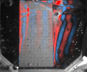
The underwater views of the cavitation pattern on the suction side of the foil are shown in figure 2 for  $\sigma _v = 0.13$ and
  $0.29$, in calm water (CW) and waves, with
  $T_w = 1.5$ s,
  $A_w = 0.05$ m,
  $\alpha = 5^{\circ }$,
  $AR_h = 1$ and
  $F_{nh} = 3.0$.

Figure 2. Underwater views of the cavitation pattern on the suction side of the foil for (a,c)  $\sigma _v = 0.13$, and (b,d)
  $\sigma _v = 0.29$, in (a,b) calm water (CW) and (c,d) waves with
  $T_w = 1.5$ s,
  $A_w = 0.05$ m; here,
  $\alpha = 5^{\circ }$,
  $AR_h = 1$ and
  $F_{nh} = 3.0$. For
  $\sigma _v = 0.13$, the flow is PC in CW and FV in waves. For
  $\sigma _v = 0.29$, both CW and wave runs are PC. Two snapshots, one at the wave crest and one at the wave trough, are shown for the wave cases in (c,d). The presence of waves causes the larger cavity to transition to FV flow, while the smaller cavity remains in the PC flow regime. In CW, the PC flow is larger for
  $\sigma _v = 0.13$ in run 2-1001 than for
  $\sigma _v = 0.29$ in run 2-4601. At
  $\sigma _v=0.13$, the turbulent, vortical flow at the cavity TE is nearer to the free surface, reducing the separation between the high-pressure gas at the free surface and the top boundary of the low-pressure PC flow. Consequently, waves tend to accelerate the transition to FV flow in the presence of a large vaporous PC flow, shown in (c), while a small PC flow can be stable in waves, such as shown in (d). Run identifiers are (a) 2-1001, (b) 2-4601, (c) 2-1201, and (d) 2-4801.
A relatively large vaporous partial cavity is present for  $\sigma _v=0.13$. The cavity, which reaches length approximately
  $L_c=0.85c$ near the mid-span, remains stable in CW, but transitions to FV flow in waves, as shown by comparing figures 2(a,c). For the CW case, the vaporous cavity has an asymmetric convex planform with cavity lengths that approach zero at the free surface and free tip because of the zero loading conditions at both sections. The cavity is relatively thin because of the sharp leading edge, which produces a well-defined detachment point. Liquid re-entrant jets form along the cavity closure line, with velocity vectors reflected about the local cavity closure line angle (see De Lange & De Bruin Reference De Lange and De Bruin1998; Laberteaux & Ceccio Reference Laberteaux and Ceccio2001; Harwood et al. Reference Harwood, Young and Ceccio2016; Young et al. Reference Young, Harwood, Montero, Ward and Ceccio2017). The tight curvature of the cavity closure line at the point of maximum length causes the re-entrant jets just above and just below to collide, which prevents the re-entrant jets from reaching the leading edge to cause complete cavity shedding. As a result, the upstream portion of the sheet cavity has a glassy surface, and only partial shedding near the cavity TE is observed. The resulting load fluctuations and deformations at the dominant cavity shedding frequency are weak. During deceleration, flow transitions back from PC to FW flow in CW, and from FV to FW in waves.
For cases in waves, shown in figure 2(c), a chance encounter of the upper boundary of the partial cavity with a wave trough produced a rapid transition to FV flow. As noted in McGregor et al. (Reference McGregor, Wright, Swales and Crapper1973), the downward acceleration of the free surface on wave backs enhances the growth of Taylor instabilities at the free surface, compromising the integrity of the surface seal. Hence waves tend to accelerate the transition from PC to FV flow. Once FV, the suction side is open to the free surface, and the foil leading edge becomes the stagnation point; a sizeable free jet spray is formed on the suction side. The ventilated cavity has an approximately triangular shape, the length of which decreases with depth as a result of increasing hydrostatic pressure. As shown in the photos, the gaseous cavity in FV flow covers nearly the entire suction side of the foil surface, and is stable. A clear ventilated tip vortex can be observed in figure 2(c), which ingests air from the ventilated suction side and base cavities.
For  $\sigma _v=0.29$, only a tiny partial cavity developed near the leading edge, regardless of the presence of waves, shown in figures 2(b,d). The maximum attached cavity length is approximately
  $0.25c$ for the CW case, and fluctuates between
  $0.20c$ and
  $0.30c$ in waves. As a result of the shortened cavity, the closure line possesses a larger radius of curvature, which leads indirectly to re-entrant flow with a more significant upstream velocity component. Consequently, periodic cavity shedding can be observed near the mid-point of the submerged span, where the liquid re-entrant jet impinges on the cavity leading edge to produce periodic shedding. However, the intensities of the load and deformation fluctuation created by unsteady cavity shedding remain small because of the cavity's limited size. The shortened cavity does not bring the cavity closure region close enough to the free surface for the free surface seal to be ruptured in the presence of waves, so the flow remains PC. Instead, waves induce oscillations in both the hydrodynamic load and cavity size because of changes in the wetted area, effective velocity field and pressure distributions. The sizes of both the vaporous and gaseous cavities tend to increase during the up-cycle of the wave (as the water level rises) and reduce during the down-cycle. At the wave crest, the horizontal component of the wave's orbital velocity increases the effective inflow velocity; at the trough, the effective inflow velocity is reduced. The vertical component of the orbital velocity points upwards during the up-cycle and downwards during the down-cycle, modifying the direction of the re-entrant jet. Note that for
  $T_w= 1.5$ s, the ratio of the wavelength to the chord is
  $\lambda _w/c' = 12.3$, where
  $c'=0.285$ m is the actual chord length, which is slightly larger than the nominal chord length
  $c = 0.279$ m because of the addition of the aluminium strip at the foil trailing edge. Wave effects are felt through the depth of the foil as
  $\lambda _w/h = 12.6$ (
 $h=0.279$ m for
  $AR_h$ = 1), although the amplitude of the wave orbital velocities decreases exponentially with
  ${\rm \pi} z/\lambda _w$, where
  $z$ is the distance from the free surface.
The time histories of the load coefficients ( $C_L, C_M, C_D$), and tip bending deformations normalized by the chord (
 $\delta /c$) and tip twist (
 $\theta$), are shown in figure 3 for the same set of runs. Figure 4 depicts the hysteresis loops formed by the moving time-averaged lift and moment coefficients (
 $C_L$ and
  $C_M$) plotted against the instantaneous Froude number (
 $F_{ni}=U_i/\sqrt {gh}$ where
  $U_i$ is the instantaneous carriage towing speed).

Figure 3. Time histories of (a i,b i,c i,d i) hydrodynamic load coefficients and (a ii,b ii,c ii,d ii) tip bending and twisting deformations for (a,c)  $\sigma _v = 0.13$ and (b,d)
  $\sigma _v = 0.29$, in (a,b) CW and (c,d) in waves with
  $T_w$ = 1.5 s,
  $A_w$ = 0.05 m. All results at
  $\alpha = 5^{\circ }$,
  $AR_h = 1$,
  $F_{nh} = 3.0$. The horizontal black dashed lines indicate SS averages. For
  $\sigma _v = 0.13$, the flow is (a) PC in CW, and (c) FV in waves. For
  $\sigma _v = 0.29$, both (b) CW and (d) wave runs are PC. The plots in (c) show a sudden drop in loading and tip deflections caused by transition from PC to FV flow, which is triggered by interactions between the vaporous cavity and waves. The mean FV loads and deformations in the SS region of (c) are much lower than those in (a) because ventilated flow reduces the peak suction pressures relative to vaporous cavitation. Run identifiers are (a) 2-1001, (b) 2-4601, (c) 2-1201, and (d) 2-4801. Here, iFV indicates the status of flow (
 $0 = {\rm FW},\ 1 = {\rm FV},\ 2 = {\rm PV},\ 3 = {\rm PC}$). iwave similarly indicates the status of waves (
 $0 = {\rm CW},\ 1 = \textrm{waves}$).

Figure 4. Hysteresis loops formed by the moving time-averaged response of the lift and moment coefficients ( $C_L$ and
  $C_M$) plotted against the instantaneous Froude number (
 $F_{ni}$). Data are shown for varying
  $\sigma _v$ with constant
  $\alpha = 5^{\circ }$,
  $F_{nh}=3.0$ and
  $AR_h=1.0$. (a,c) Calm water and (b,d) wave (
 $T_w=1.5$ s and
  $A_w=0.05$ m) runs, indicated by the tags
  $iwave=0$ and
  $iwave=1$. The dominant flow regimes are indicated by line colour, as denoted in the legends. Load coefficients are similar across all of the runs during the acceleration phase until a sufficiently large partial cavity develops (
 $\sigma _v = 0.13$), which leads to a slight increase in
  $C_L$ due to virtual camber effect and a slight decrease in
  $C_M$ due to the shift in centre of pressure towards the mid-chord. Large reductions in
  $C_L$ and
  $C_M$ for all the wave cases with
  $\sigma _v=0.13$ in (b,d) result from wave-induced transition from PC to FV flow. Once FV, the atmospheric ventilated cavity persists during deceleration until
  $F_{ni} \approx 1.5$, forming a large hysteresis loop.
For  $\sigma _v=0.13$, the leading edge vaporous cavity (PC flow) produces an increase in
  $C_L$ due to a virtual camber effect, along with a slight reduction in
  $C_M$ due to shifting of the centre of pressure towards the mid-chord, when compared to the smaller cavity at
  $\sigma _v=0.29$. In waves, the transition of the larger cavity from PC to FV flow is accompanied by a dramatic reduction in the hydrodynamic forces and structural response in figure 3(c), as well as the plots on the right-hand side of figure 4. Transition from PC to FV flow caused a 70 % drop in
  $C_M$ but only a 40 % drop in
  $C_L$. Once FV, the gas cavity persists during deceleration until
  $F_{ni}\approx 1.5$, producing the large hysteresis loops observed on the right-hand side of figure 4. In addition, note the direct correlation between
  $C_L$ and
  $\delta$ and between
  $C_M$ and
  $\theta$ for all the cases, including the sudden transition from PC to FV flow in figure 4(c) and the wave-induced oscillations in figure 4(c,d). The apparent linearity of the structural response suggests that, although the deformations are small, they can be used to effectively infer the hydrodynamic loads, which has been discussed in Ward, Harwood & Young (Reference Ward, Harwood and Young2018).
Comparison of the hysteresis loops in figure 4 for different values of  $\sigma _v$ shows that the forces are very similar in the acceleration phase for all runs, with only a slight increase in
  $C_L$ and a slight decrease in
  $C_M$ when a sufficiently large partial cavity develops (attributed to the camber-like deflections in suction-side streamlines). Differences between the CW cases in figures 4(a,c) and the wave cases in figures 4(b,d) are most evident in the significant drops in
  $C_L$ and
  $C_M$ when flow transitions from PC to FV, and the large hysteresis loop caused by the delay in flow re-attachment. The differences in the hysteresis loops shown for the CW cases in figures 4(a,c) and the wave cases in figures 4(b,d) indicate clearly that waves tend to accelerate transition to FV flow when a sufficiently large partial cavity is present. This is supported by figure 2. On the other hand, when a smaller partial cavity is present (
 $\sigma _v=0.29$), or in subcavitating flow (
 $\sigma _v=8$), waves produce oscillatory loading with the same slowly varying mean as in CW, consistent with the findings of Part 1.
Figure 5 depicts the joint time–frequency analysis of the tip twist deformations ( $\theta$) for the same runs depicted in the preceding figures. For each panel, the top plot shows the time history of
  $\theta$ (solid blue line) and the instantaneous Froude number
  $F_{ni}$ (red dashed line), the lower left plot contains the power spectrum (PS) of
  $\theta$, and the lower right plot depicts the WSST of
  $\theta$ in time–frequency space. As in previous figures, CW results are shown in figures 5(a,b), wave results are in figures 5(c,d), results for
  $\sigma _v=0.13$ are in figures 5(a,c), and results for
  $\sigma _v=0.29$ are in figures 5(b,d). The results for all three PC runs are quite similar in figures 5(a,b,d). Conversely, the transition from PC to FV flow with the larger vaporous cavity in waves is signalled by an impulse-like signature near the end of the acceleration stage in figure 5(c) (at approximately 16 s). The time–frequency spectra of all four runs are marked by a peak in spectral energy that tracks the dashed red line corresponding to a constant Strouhal number of
  $St=0.265$, indicating that TE vortex shedding is present at all speeds. Peaks can also be observed at the foil modal frequencies
  $f_1, f_2, f_3$, the carriage modal frequency
  $f_{car}$, and the vortex shedding frequency
  $f_{vs}$. The dominant frequency for the cases with waves is the wave encounter frequency
  $f_e$.

Figure 5. Time–frequency spectra of the tip twist deformation ( $\theta$) for (a,c)
  $\sigma _v=0.13$ and (b,d)
  $\sigma _v=0.29$, in (a,b) CW and (c,d) waves with
  $T_w=1.5$ s and
  $A_w=0.05$ m, for
  $\alpha = 5^{\circ }$,
  $AR_h=1$,
  $F_{nh}=3.0$. In each panel, the top plot shows the time history of
  $\theta$ (solid blue line) and the instantaneous Froude number
  $F_{ni}$ (red dashed line), the lower left plot indicates the power spectrum (PS) of
  $\theta$, and the lower right plot indicates the time–frequency spectrum of
  $\theta$. The cyan triangles on the
  $y$-axes of the lower plots mark the first three modal frequencies of the hydrofoil. The green crosses indicate the carriage frequency. The vortex shedding frequency (
 $\,f_{vs}$) is indicated by the magenta dashed line, and the wave encounter frequency (
 $\,f_e$) is indicated by the red dotted line. For
  $\sigma _v=0.13$, the flow is PC in CW and FV in waves. In (c), the transition from PC to FV flow is evident via the drop in
  $\theta$ (caused by a drop in moment) along with an impulse-like signature in the time–frequency spectra at
  $\approx$ 17 s. For
  $\sigma _v=0.29$, both CW and wave runs are PC (as observed in the underwater images in figures 2b,e, f) and share similar time–frequency spectra except for the addition of the dominant peak at
  $f_e$ for the wave cases in (c,d). Run identifiers are (a) 2-1001, (b) 2-4601, (c) 2-1201, and (d) 2-4801.
5.2. Influence of $\sigma _v$ and waves with large immersed aspect ratio

Figure 6 depicts the underwater views of the foil's suction surface and the associated load and deformation time histories. Runs under consideration include  $\sigma _v = 0.25$ in CW (figures 6a,b),
  $\sigma _v=0.25$ in waves with
  $T_w = 1.5$ s and
  $A_w = 0.05$ m (figures 6c,d), and
  $\sigma _v = 0.80$ in CW (figures 6e, f). All runs are at
  $\alpha = 5^{\circ }$,
  $AR_h = 2$ and
  $F_n = 1.5$. The time–frequency spectra of the tip twist deformation (
 $\theta$) for these runs are shown in figure 7.

Figure 6. (a,c,e) Underwater views of the cavitation pattern on the suction side of the foil. (b,d, f) Time histories of hydrodynamic load coefficients ( $C_L$,
  $C_M$ and
  $C_D$) and tip deformations (
 $\delta /c$ and
  $\theta$). Results are shown for (a,b) run 2-3001,
  $\sigma _v=0.25$ in CW, (c,d) run 2-2301,
  $\sigma _v=0.25$ for waves, with
  $T_w=1.5$ s and
  $A_w=0.05$ m, and (e, f) run 2-5001,
  $\sigma _v=0.80$ in CW. Horizontal black dashed lines indicate the average values in the SS region. Compared to the results for
  $AR_h = 1$ in figure 2, loads are higher for
  $AR_h = 2$ because three-dimensional effects are reduced, and the amplitude of fluctuations is larger due to frequency coalescence of modes 2 and 3. All three cases are PC, but the cavities are longer for (b,d) with
  $\sigma _v=0.25$ than for (e) with
  $\sigma _v=0.80$. The von Kármán vortex in the lower submerged tip portion of the foil is more obvious for
  $\sigma _v=0.25$ because of the vapour/gas mixture formed by the interaction between the shed vaporous cavities and the aerated separated region. Vaporous cavity shedding in (a,c) for
  $\sigma _v=0.25$ modulates the aerated vortex street.

Figure 7. Time–frequency spectra of the tip twist deformation ( $\theta$) for (a) run 2-3001,
  $\sigma _v=0.25$ in CW, (b) run 2-3201,
  $\sigma _v=0.25$ for waves, with
  $T_w=1.2$ s and
  $A_w=0.05$ m, and (c) run 2-5001,
  $\sigma _v=0.80$ in CW, for
  $\alpha = 5^{\circ }$,
  $AR_h=2$,
  $F_{nh}=1.5$. In each panel, the top plot shows the time history of
  $\theta$ (solid blue line) and the instantaneous Froude number
  $F_{ni}$ (red dashed line), the lower left plot indicates the power spectrum (PS) of
  $\theta$, and the lower right plot indicates the time–frequency spectrum of
  $\theta$. The cyan triangles on the
  $y$-axes of the lower plots mark the first three modal frequencies of the hydrofoil. The green crosses indicate the carriage frequency. The vortex shedding frequency (
 $\,f_{vs}$) is indicated by the magenta dashed line, and the wave encounter frequency (
 $\,f_e$) is indicated by the red dotted line. For the CW case with
  $\sigma _v = 0.80$ in (c), the dominant frequency is 28 Hz, where modes 2 and 3 coalesced, and is slightly below
  $f_{vs}$. On the other hand, lock-in with the cavity shedding frequency for
  $\sigma _v = 0.25$ caused the dominant peak to shift to 30.5 Hz. Comparison between (a,b) shows evidence of wave-induced modulation of the foil modal frequencies and vortex shedding frequency.
As shown in figure 6, all three cases have small, vaporous leading edge cavities, which are slightly longer for  $\sigma _v=0.25$ (
 $L_c/c\approx 0.25$) than for
  $\sigma _v=0.80$ (
 $L_c/c<0.09$). The cavity in figure 6(c) is so small that it is barely visible. Higher mean loads and deformations are evident in figures 6(d–f) compared to figure 2 as a result of a larger immersed span and reduced three-dimensional effects. None of the cavities is large enough to produce a meaningful change in the mean hydrodynamic loads or elastic deformations. At
  $AR_h=2.0$, the natural frequencies of modes 2 and 3 are nearly identical, producing a phenomenon known as frequency coalescence. As a result of dynamic load amplification caused by this coalescence, the amplitudes of fluctuating hydrodynamic forces and deflections are also much higher at
  $AR_h = 2$ than at
  $AR_h = 1$. Frequency coalescence will be discussed at length later in this section when presenting results from the co-analysis of the structural and hydrodynamic modes.
The blunt TE of the foil produces an aerated separated region. The differential shear flow from the suction and pressure sides of the TE leads to periodic von Kármán vortex shedding that follows the Strouhal law and can be observed with the naked eye because the vortex cores entrain air from the TE flow, as well as bubbles generated from upstream vaporous cavity shedding. The vortex cores appear as inclined striations in the foil's wake, which are more readily visible for  $\sigma _v=0.25$ because of the increased generation of bubbles by the larger partial cavity.
The time–frequency spectra of the tip twist deformation in figure 7 show high intensities for all three runs at constant Strouhal numbers, as identified by the magenta dashed line. Periodic shedding of a vaporous cavity cloud was also observed to interact with the von Kármán vortex, leading to the formation of heterodyne frequencies at the sums and differences of the cavity shedding frequency and the vortex shedding frequency. In addition, waves produced periodic modulation of the cavity sizes and thus cavity shedding frequency, which in turn altered the interaction of cavity shedding with the von Kármán vortex shedding and lock-in with the foil modal frequencies. Wave-induced frequency and amplitude modulation of the modal frequencies (particularly  $f_{2}$ and
  $f_{3}$), cavity shedding frequency and vortex shedding frequency (
 $\,f_{vs}$) are evident in figure 7(b), where small fluctuations can be observed about
  $f_{vs}$ and the modal frequencies. Comparison of the time–frequency spectra shown in figure 7 for
  $AR_h=2$ versus those in figure 5 for
  $AR_h=1$ clearly illustrates the extremely energetic response that accompanies the coalescence of modes 2 and 3 so near
  $f_{vs}$ at
  $AR_h=2$.
Figure 8 shows the PSD plots of the fluctuating lift coefficient ( $C_L$) and the tip bending displacement (
 $\delta )$. Calm water cases are shown in figures 8(a,c), and runs in waves in figures 8(b,d). In addition to the three runs depicted in figure 6, data are also included for a range of values of
  $\sigma _v$ that includes subcavitating conditions (
 $\sigma _v=15.93$). At
  $\sigma _v=0.80$, the very short partial cavity (
 $Lc/c<0.09$) has a negligible influence on the dynamic response, producing a spectrum almost indistinguishable from that of the FW flow of run 1-2202 (
 $\sigma _v=15.94$, also presented in Part 1). PSD plots for
  $\sigma _v>0.5$ in CW and waves show a significant peak near 28 Hz where coalescence of modes 2 and 3 occurs. The peak corresponding to
  $f_2$ and
  $f_3$ shifts up slightly as
  $\sigma _v$ decreases, falling near 30.5 Hz for
  $\sigma _v=0.25$. Following the Strouhal law based on the relative inflow velocity and the maximum attached cavity length, the cavity shedding frequency decreases as the cavity lengthens. For
  $\sigma _v=0.25$, the cavity shedding frequency appears to be locked in with
  $f_{3}$ at 30.5 Hz. Here,
  $f_{vs}$ is largely unaffected by changing values of
  $\sigma _v$. For all cases in waves, a significant peak can be observed at the wave encounter frequency
  $f_e$, which is 2.33 Hz for run 2-3201 with
  $T_w=1.2$ s, and 1.67 Hz for the other wave runs with
  $T_w=1.5$ s. Wave-induced frequency modulations are evident via smaller peaks at
  $f_{2}\pm nf_e$,
  $f_{3}\pm nf_e$ and
  $f_{vs}\pm nf_e$, with
  $n=1,2$.

Figure 8. Power spectral density (PSD) plots of (a,b) the fluctuating lift coefficient ( $C_L$), and (c,d) the tip bending displacement (
 $\delta$), for various values of
  $\sigma _v$ with fixed
  $\alpha = 5^{\circ }$,
  $F_{nh}=1.5$,
  $AR_h=2.0$. (a,c) CW, and (b,d) wave runs (
 $A_w=0.05$ m,
  $T_w=1.5$ s for all the cases except for 2-3201 with
  $T_w=1.2$ s). The FW and PC results are shown as thin solid and thin dash-dotted lines, respectively. The carriage (
 $\,f_{car}$) and FW foil modal frequencies (
 $\,f_{1,FW}^*$ to
  $f_{4,FW}^*$) are indicated by the vertical green and red dashed lines, respectively. The vortex shedding frequency (
 $\,f_{vs}$) is shown as the vertical maroon dashed line. The foil modal frequencies increase with decreasing
  $\sigma _v$, but they are not shown to avoid over-cluttering the graphs. The wave encounter frequency (
 $\,f_e$) is 2.33 Hz for run 2-3201, and 1.67 Hz for the other wave runs. For PC or FW flow such that
  $\sigma _v \geq 0.8$, the primary peak is at 28 Hz due to frequency coalescence of modes 2 and 3. For
  $\sigma _v = 0.35$ and 0.5, cavity shedding leads to frequency modulations, leading to slightly lower peak amplitude. For
  $\sigma _v = 0.25$, lock-in of the cavity shedding frequency with the foil modal frequency caused the primary peak to shift to the right, and the amplitude and sharpness of the peak are approximately the same. The shifts of the peak frequency caused by lock-in with the cavity shedding are also visible via its harmonic visible near 60 Hz. Compared to the CW cases in (a,c), additional small peaks can be observed near the modal frequencies and vortex shedding frequency for the wave cases in (b,d).
Output-only SSIs of the structural motions, paired with the SPODs of the high-speed video records, were used for the co-analysis of structural and hydrodynamic modes. While the preceding joint time–frequency spectra and PSD plots of lift and bending effectively show the evolution of spectral energies in time and across conditions, the aim of the co-analysis is to identify with greater certainty the energetic processes associated with each peak. In so doing, we can confirm the frequency coalescence of modes 2 and 3, and lock-in with the cavity shedding frequency, as well as interplay between foil modal excitation, cavity shedding frequency, vortex shedding frequency and wave encounter frequency.
Table 2 summarizes the parameters identified for the three runs under consideration. As described in § 3.2, each entry represents a complex pole of the fitted state-space model. Each pole has been classified as a forced response to a hydrodynamic excitation (E), a hydrofoil resonance (R), or a spurious mode resulting from over-fitting of spectral noise. Classifications were made by considering the structural auto-power spectral densities, resulting mode shapes, and the concurrent videographic modes, which are presented for run 2-3001 ( $\sigma _v=0.25$, CW) in figure 9, run 2-3201 (
 $\sigma _v=0.25$, waves) in figure 10, and run 2-5001 (
 $\sigma _v=0.80$, CW) in figure 11. For all three runs, the coalescence of modes 2 and 3 near 28 Hz is apparent, but the proximity of the leading edge cavity shedding (CS) will be shown in the following figures to result in lock-in with one or both modes.

Figure 9. Co-analysis results for a high aspect ratio in CW: run 2-3001 with  $\alpha =5^\circ$,
  $F_{nh}=1.5$,
  $AR_h=2.0$,
  $\sigma _v=0.25$, PC flow. (a) Tip bending and twisting auto-power spectral densities (measured and fitted with SSI). Blue dash-dotted lines indicate the modal frequencies anticipated from historical results. The red dashed line is the theoretical vortex shedding frequency (
 $St=0.265$). Black dashed lines indicate poles fitted using the SSI algorithm. (b) Results of co-analysis. For each pole, the top row shows the visually observable hydrodynamic mode, and the bottom row shows the structural mode or ODS produced by SSI at the same frequency. Structural modes are not generally accompanied by coherent hydrodynamic modes, while forced vibration responses, like that at the vortex shedding frequency, show clearly defined hydrodynamic modes. The prominent peak at 30.5 Hz, and the dominance of partial cavity shedding in the hydrodynamic mode, combined with the apparent mix of bending and torsion deformations in the hydrofoil, suggest that mode 2 and/or mode 3 experienced lock-in with the nearby LE cavity shedding. The presence of vertical striations in the wake of the hydrofoil at both 30.5 and 33 Hz suggests that vortical structures are shedding from the TE as a result of both the structural vibrations at 30.5 Hz and the conventional von Kármán vortex street. Supplementary movie 1 contains animations of each mode.

Figure 10. Results for run 2-3201:  $\alpha =5^\circ$,
  $F_{nh}=1.5$,
  $AR_h=2.0$,
  $\sigma _v=0.25$, PC flow; waves with
  $T_w = 1.5$ s and
  $A_w = 0.05$ m. (a) Tip bending and twisting auto-power spectral densities (measured and fitted with SSI). (b) Results of co-analysis. Waves lead to modulations of the foil's resonant frequencies, evident as side-bands in the spectra. The spacing between
  $f_2$ and
  $f_3$, the cavity shedding (CS) frequency, and
  $f_{VS}$ matches closely the encounter frequency
  $f_e$, apparently driving intermittent lock-in between modes 2 and 3 and the LE CS as
  $f_2, f_3$ modulate. Supplementary movie 2 contains animations of each mode.

Figure 11. Results for run 2-5001:  $\alpha =5^\circ$,
  $F_{nh}=1.5$,
  $AR_h=2.0$,
  $\sigma _v=0.80$, PC flow, CW. (a) Tip bending and twisting auto-power spectral densities (measured and fitted with SSI). (b) Results of co-analysis. A single pole is fitted to the coalescent modes near
  $f_2$ and
  $f_3$, which are apparently dominating the lock-in with the LE cavity shedding. The associated SPOD mode shows a thin but energetic fluctuation at the hydrofoil's LE, signalling that the LE cavity shedding (with a cavity length shorter than in run 2-3001) is synchronous with the vibration of modes 2 and 3. The hydrodynamic mode shows only weak vortical structures in the hydrofoil's wake, suggesting little interaction between modes 2 and 3 and the von Kármán vortex street, unlike run 2-3001. Supplementary movie 3 contains animations of each mode.
Table 2. Tabulations of undamped natural frequency ( $\,f_0$), damped natural frequency (
 $\,f_n$), and percentage critical damping (
 $\xi$) for each of the modes produced by the SSI algorithm. Results are shown for two CW conditions (
 $\sigma_v=0.25$, run 2-3001 and
  $\sigma_v=0.80$, run 2-5001) and one wave condition (
 $\sigma_v=0.25$, run 2-3201). All conditions are at
  $\alpha =5^\circ$,
  $AR_h=2.0$,
  $F_{nh}=1.5$. A combination of the structural mode shapes and concurrent hydrodynamic modes (shown in figures 9–11) was used to classify each mode as an (E)xcitation, (R)esonance, or spurious mode. CS denotes cavity shedding. Notable quantities include the more than two orders of magnitude difference in
  $\xi$ for mode 2/3 for run 2-5001 with
  $\sigma _v=0.8$ compared to run 2-3001 with
  $\sigma _v=0.25$, where both runs are in CW. The single dominant damped frequency at 28.78 Hz identified for modes 2 and 3, and the 0.10 % damping coefficient for run 2-5001, suggest modal coalescence. On the other hand, lock-in with leading edge (LE) cavity shedding frequency caused the dominant peak for run 2-3001 to be shifted to 30.47 Hz, which has a lower
  $\xi$ value of 0.05 %. In run 2-3201 with waves, the dominant frequency is approximately the same at 30.46 Hz, but
  $\xi =0.20\,\%$ due to wave-induced frequency and amplitude modulations.

The fitted spectra for  $\sigma _v=0.25$ in CW are shown in figure 9(a), overlaid with blue dash-dotted lines to denote anticipated modal frequencies
  $f_1$ to
  $f_4$, a red dashed line to indicate the von Kármán vortex shedding frequency with Strouhal number
  $St=0.265$, and black lines to denote modes fitted using SSI and reported in table 2. Figure 9(b) shows, for a selection of modes with less than 50 % damping, the structural mode or operating deflection shape (bottom row) and the most energetic SPOD mode at the same frequency (top row). For complex modes like those produced by SSI, node lines change in time, and phase information is lost in plotting only the real part of the mode shapes. For each SSI pole, the complex mode shape was rotated to maximize the Euclidean norm of its real part, which was shown by Ahmadian, Gladwell & Ismail (Reference Ahmadian, Gladwell and Ismail1995) to maximize the similarity between a complex mode and its associated (real) normal mode shape. An animated version of the same figure is included as a supplementary movie available at https://doi.org/10.1017/jfm.2023.254, which consists of the full complex mode (travelling wave solution) over several cycles.
The first SSI mode in figure 9(b) confirms that mode 1 is a simple cantilever bending mode shape. A single pole was detected near 27 Hz – the expected coalescence frequency of modes 2 and 3 – but lacks a prominent peak, which causes a relatively large damping estimate in table 2. The much larger peak in the spectra at 30 Hz suggests that a proximate excitation is driving the coalescent modes at the very least – and probably producing lock-in with one or both modes. The leading edge (LE) vaporous cavity is too short to produce a very intense excitation on its own, so the prominent peak at the cavity shedding frequency offers compelling evidence that lock-in of the cavity shedding frequency is occurring with modes 2 and 3. This notion is reinforced both by the low damping in table 2 and by the structural ODS at 30.5 Hz, which shows evidence of the mixed first-torsion and second-bending mode shapes. Here, we refer to the SSI mode as an ODS – a periodic structural response excited by a coherent excitation, representing a mixture of nearby mode shapes. The detection of a pole at 27.5 Hz implies that lock-off occurred for a portion of the steady-state duration. The SPOD hydrodynamic mode at 30.5 Hz shown in the top row of figure 9(b) clearly shows two regions of concentrated fluctuation – one in the LE partial cavity, and one in the hydrofoil wake. This implies that cavity shedding at the LE interacts with the von Kármán vortex street through the resonant vibrations, producing vortical structures along the entire submerged span. At 33 Hz, we see a stronger TE vortex shedding pattern which is concentrated along the shallower portion of the hydrofoil's span, indicative of von Kármán vortex shedding from the TE of the base-ventilated cavity.
As waves are introduced and the cavitation number held at  $\sigma _v=0.25$, the effects of wave modulation appear in figure 10(a) as side-bands flanking the most dominant peaks at distances
  $\pm f_e$, and in the hydro-structural modes of figure 10(b) as overlapping ranges of frequencies assigned to each physical process. The wave encounter frequency
  $f_e=2.25$ Hz is identified clearly, producing an ODS almost indistinguishable from the first bending mode at
  $f_1$. At
  $f_e$, the negative estimated damping (see table 2) reflects the sharply concentrated peak in the excitation spectrum. While the quantitative damping estimate is suspect, it reflects correctly that the input spectrum possesses the same sharp peak. Another peak near 28 Hz once again appears to match the coalescence of
  $f_2$ and
  $f_3$. Compared to the CW case, the reduction in damping at the coalescence frequency reflects the increased energy at
  $f_2, f_3$. We posit that the wave-modulated resonant and cavity shedding frequencies resulted in a periodic lock-in and separation of modes 2 and 3 with the cavity shedding process. This is consistent with the periodic shifts in the spectral energy of figure 7.
As in CW, the LE vaporous cavity resides halfway between the coalescence frequency of  $f_2,f_3$ and the vortex shedding frequency
  $f_{vs}$. Both the first twisting (mode 2) and second bending (mode 3) shapes are evident in all three of the structural ODS. Moreover, the separation distance between each peak closely matches the wave encounter frequency
  $f_e$, which makes it even more likely that intermittent lock-in occurred between the cavity shedding frequency and modes 2 and 3. Secondary peaks appear near
  $f_{vs}$ as well, which confirms that the vortex spacing is affected to some degree by the presence of waves (and the periodic changes in effective convective speed) and by structural vibrations.
Figure 11 shows the co-analysis results for a higher cavitation number  $\sigma _v=0.8$, which produces only a very short LE vaporous cavity, as is evident from figure 6(c) and via the third plot from the left on the hydrodynamic modes shown on the top row of figure 11(b). Unlike the preceding two cases, only a single mode pole is fitted in the proximity of
  $f_2,f_3$ and the apparent cavity shedding frequency. At the higher cavitation number
  $\sigma _v=0.8$, the shorter cavity should experience higher-frequency shedding than at
  $\sigma _v=0.25$. The opposite is true, however, and we see a thin region of colouration along the LE of the hydrodynamic mode at 28.8 Hz, indicating that the LE cavity shedding is synchronous with coalescent modes 2 and 3. Therefore, lock-in is still occurring, but the weak excitation and the minimal changes in added mass produced by such a short cavity result in a lock-in frequency much closer to the FW coalescence frequency of modes 2 and 3. Hence the co-analysis results shown in figures 9–11 support the earlier statement that the shifting of the dominant peak to the right of 28 Hz in the PSD plots shown in figure 8 is caused by cavity-induced lock-in for cases with
  $\sigma _v=0.25$. Comparison of the results for
  $\sigma _v=0.8$ shown in figure 11 with that of
  $\sigma _v=0.25$ in figure 9 also indicates that while the vortex shedding pattern appears almost identical, there is no strong interaction evident between the LE cavity and the TE vortex street, i.e. the vortical structures aft of the TE are very weak at 28.8 Hz.
5.3. Influence of varying wave amplitude and steepness
Figure 12 shows underwater views of the cavitation patterns on the suction side of the hydrofoil for three runs, respectively in CW and with wave amplitudes  $A_w = 0.05$ m and 0.10 m. The same wave period
  $T_w = 1.5$ s was maintained for both runs in waves to illustrate the effects of varied wave steepness. All runs share conditions
  $\sigma _v = 0.3$,
  $\alpha = 5^{\circ }$,
  $AR_h = 1$ and
  $F_{nh} = 3.5$. The corresponding time histories of the loads and deformations are shown in figures 12(b,d, f). The time–frequency spectra of the tip twist deformation (
 $\theta$) for these runs are shown in figure 13. Figure 14 shows the hysteresis loops formed by the moving time-averaged response of the lift and moment coefficients (
 $C_L$ and
  $C_M$) versus the instantaneous Froude number (
 $F_{ni}$) for the same set of runs. The corresponding PSD plots of the fluctuating lift coefficient (
 $C_L$) are shown in figure 15(a), and tip bending displacement (
 $\delta )$ in figure 15(b).

Figure 12. (a,c,e) Underwater views of the cavitation patterns on the suction side of the foil, and (b,d, f) time histories of hydrodynamic load coefficients ( $C_L$,
  $C_M$ and
  $C_D$) and tip deformations (
 $\delta$/c and
  $\theta$). Plots are shown for (b) a CW run, (d) a wave run with wave amplitude
  $A_w=0.05$ m, and ( f) a wave run with wave amplitude
  $A_w=0.10$ m, with
  $T_w=1.5$ s,
  $\sigma _v=0.30$,
  $\alpha = 5^{\circ }$,
  $AR_h=1$ and
  $F_{nh}=3.5$. The horizontal black dashed lines in the time history plots indicate the average values in the SS region. The flow is PC in the CW case and in the wave case with
  $A_w=0.05$ m. When
  $A_w=0.10$ m, the steeper wave with higher wave orbital velocity can puncture the surface seal to reach the longer vapour cavity just beneath, forcing the flow to transition from PC to FV flow near 14 s, as evidenced by the large ventilated cavity in (e) and the sudden large drop in loads and deformations in ( f). (a,b) Run 2-5801,
  $\sigma _v = 0.3$, CW. (c,d) Run 2-6001,
  $\sigma _v = 0.3$, waves,
  $A_w = 0.05$ m. (e,f) Run 2-6201,
  $\sigma _v = 0.3$, waves,
  $A_w = 0.10$ m.

Figure 13. Time–frequency spectra of the tip twist deformation ( $\theta$) for (a) CW run 2-5801, (b) run 2-6001, waves,
  $A_w=0.05$ m,
  $T_w=1.5$ s, and (c) run 2-6201, waves,
  $A_w=0.1$ m
  $T_w=1.5$ s. All runs share parameters
  $\sigma _v=0.30$,
  $\alpha = 5^{\circ }$,
  $AR_h=1$ and
  $F_{nh}=3.5$. In each panel, the top plot shows the time history of
  $\theta$ (solid blue line) and the instantaneous Froude number
  $F_{ni}$ (red dashed line), the lower left plot indicates the power spectrum (PS) of
  $\theta$, and the lower right plot indicates the time–frequency spectrum (WSST) of
  $\theta$. The cyan triangles on the
  $y$-axes of the lower plots mark the first three modal frequencies of the hydrofoil. The green crosses indicate the carriage frequency. The vortex shedding frequency (
 $\,f_{vs}$) is indicated by the magenta dashed line, and the wave encounter frequency (
 $\,f_e$) is indicated by the red dotted line. Comparison between the three plots shows that waves produced frequency and amplitude modulations, which cause the peaks in the power spectra to appear ‘spread out’, thus appearing to have higher damping or low intensity at the foil modal frequencies. The case with the steep waves accelerated the transition from PC to FV flow at approximately 14 s, signalled by the impulse-like signature in the time–frequency spectra and the sudden drop in
  $\theta$ in the time history plot in (c).

Figure 14. Hysteresis loops formed by the moving time-averaged response of the lift and moment coefficients ( $C_L$ and
  $C_M$) plotted against the instantaneous Froude number (
 $F_{ni}$) in CW and waves of varying steepness. All runs share parameters
  $\sigma _v=0.30$,
  $\alpha = 5^{\circ }$,
  $AR_h=1$ and
  $F_{nh}=3.5$. The hysteresis loops for the two PC runs are counter-clockwise because the unsteady circulatory lift lags the instantaneous speed, augmented by the virtual camber effect of the hysteretic LE cavity. The hysteresis loop for the FV run is clockwise and much larger because of the large reduction in loading during the transition from PC to FV flow. Nevertheless, the acceleration portion of the hysteresis loop is almost identical between the three runs until the LE partial cavity grew large enough to interact with the steepest waves, which occurred near the target steady Froude number
  $F_{nh} = 3.5$.

Figure 15. Comparison of the PSD of the fluctuating components of (a) lift coefficient ( $C_L$), and (b) tip bending displacement (
 $\delta$). Traces show runs in CW and waves of varying steepness, all with
  $\sigma _v=0.30$,
  $\alpha = 5^{\circ }$,
  $AR_h=1$ and
  $F_{nh}=3.5$. The PC and FV results are shown as thin dash-dotted lines and thick solid lines, respectively. The carriage (
 $\,f_{car}$) and FW foil modal frequencies
  $f_{1,FW}^*$ to
  $f_{4,FW}^*$ are indicated by the vertical green and red dashed lines, respectively. The vortex shedding frequency (
 $\,f_{vs}$) is shown as the vertical maroon dashed line. The wave encounter frequency
  $f_{e}$ is 2.31 Hz for the two wave cases. The PSD plots of the three runs are very similar except for the addition of a peak at
  $f_e$ and a general increase in the intensity of the
  $\delta$ fluctuations for
  $f>10$ Hz for the wave cases. Although run 2-6201 with
  $A_m=0.10$ m is FV, the PSD looks very similar to run 2-6001 with
  $A_m=0.05$ m in PC flow.
In figure 12, the PC flow appears qualitatively similar in CW and in shallow waves, characterized by a long LE vaporous cavity ( $L_c/c \approx 0.6$ in CW, and
  $L_c/c \approx 0.7$ in waves). While slightly longer, the partial cavity in waves is also less stable, with a re-entrant jet that changes direction periodically as orbital wave velocities alter the local inflow angle. The hydrodynamic loads and tip deformations are approximately equal in the mean, but with superimposed fluctuations at the encounter frequency evident in 2-6001. The combination of shallow immersion depth and high speed additionally produces a large base cavity that extends to the free tip. By enclosing the blunt TE in a gaseous cavity, the development of opposing shear layers in the wake – and the associate vortex street – is suppressed, so the characteristic striations in the foil's wake are absent. In the steeper waves, with
  $A_w=0.10$ m, the larger wave orbital velocities and surface accelerations produce instabilities on the free surface seal that allow air to enter the large vapour-filled cavity, initiating the sudden transition from PC to FV flow near 14 s. Transition results in the large ventilated cavity in figure 12(c) and the sudden large drop in loads and deformations in figure 12( f).
Figure 13 shows that, compared to the CW case in figure 13(a), the presence of small-amplitude waves in figure 13(b) led to the addition of a dominant peak at  $f_{e}$, as well as frequency and amplitude modulation of
  $f_2$,
  $f_3$ and
  $f_{vs}$. The peaks in figure 13(b) are less distinct than those in figure 13(a) as a result of the modulation in natural frequencies and cavity shedding produced by waves. For the steeper waves with amplitude
  $A_w=0.10$ m, the flow transitioned from PC to FV near 14 s. The sudden change in loading during transition produces an impulse-like signature in the time–frequency spectrum. The energy around
  $f_{vs}$ is most apparent during the acceleration and deceleration phases, where the base cavity (or, in the case of run 2-6201, the ventilated cavity) does not suppress the TE vortex street.
The hysteresis loops with respect to  $F_{ni}$, shown in figure 14, move in a counter-clockwise direction in PC flow because the circulatory lift, the circulatory moment and the length of the partial cavity lag slightly behind the instantaneous speed as a result of wake memory effects. The unsteady circulatory lift is augmented by the size of the cavity, which produces a slight camber on the suction surface. Curiously, the hysteresis loop in waves with small amplitude (
 $A_w=0.05$ m) is much smaller, even though the flow regime remains PC throughout the run. Two explanations are hypothesized for this behaviour. First, the slightly greater length of the partial cavity in waves may actually reduce the curvature of the flow over the suction surface (the virtual camber), consistent with the flat-plate solution of Acosta (Reference Acosta1973). Second, the increased shedding produced by the interaction of the re-entrant flow with orbital wave velocities produces some local flow separation near the cavity closure that counteracts some of the expected lift augmentations by the partial cavity. With large amplitude or steep waves, the PC flow transitions to FV, which persists to much lower speeds than the PC flow before re-wetting; the hysteresis area is much larger than either of the two preceding cases as a result.
In figure 15, a comparison of the PSD plots of the three runs shows that increasing wave amplitude increases the overall energy content. Still, waves do not affect the location of the peaks of the frequency spectra except for the addition of a peak at  $f_{e}$, and modulation of the peaks at
  $\pm nf_{e}$, with
  $n = 1,2$. As noted in the previous section, FV flow – this time produced by steep waves – does alter the locations and intensities of several peaks. Additional insight into the character and origin of spectral peaks is gained from the SSI-SPOD co-analysis, the results of which are presented in table 3. Fitted spectra and hydrodynamic and structural modes are presented for runs 2-5801 in figure 16, 2-6001 in figure 17 and 2-6201 in figure 18. At the immersed aspect ratio
  $AR_h=1.0$, modes 2 and 3 are well separated, so the ambiguity in mode shapes observed at
  $AR_h=2.0$ is absent. The damping of both modes is higher across all three runs than the damping of the combined/coalescent mode fitted when
  $AR_h=2.0$. A comparison between runs 2-5801 (in table 3) and 2-3001 (in table 2) shows the dramatic difference in modal added mass between
  $AR_h=1.0$ and
  $AR_h=2.0$, with a change in
  $f_3$ of approximately 20 Hz. No cavity shedding was identified at
  $AR_h=1.0$ because at shallower depths, the oblique cavity closure lines prevent organized shedding driven by the re-entrant jet. The large base cavity suppresses the development of a von Kármán vortex street in the wake of the TE, so no vortex shedding excitation is detected, either.

Figure 16. Results for run 2-5801:  $\sigma _v=0.30$,
  $\alpha = 5^{\circ }$,
  $AR_h=1$ and
  $F_{nh}=3.5$; PC flow, CW. (a) Tip bending and twisting auto-power spectral densities (measured and fitted with SSI). (b) Results of co-analysis. Resonance modes are well separated from one another and from excitations. As a result, none of the hydrodynamic modes associated with
  $f_1$,
  $f_2$ and
  $f_3$ shows coherent visible flow structures. Furthermore, neither the LE cavity shedding nor the TE vortex shedding produces responses that are energetic enough to be identified by the SSI algorithm. Supplementary movie 4 contains animations of each mode.

Figure 17. Results for run 2-6001:  $\sigma _v=0.30$,
  $\alpha = 5^{\circ }$,
  $AR_h=1$ and
  $F_{nh}=3.5$; PC flow, waves with
  $T_w=1.5$ s and
  $A_w=0.05$ m. (a) Tip bending and twisting auto-power spectral densities (measured and fitted with SSI). (b) Results of co-analysis. Aside from a slight increase in the frequency of the pole fitted to mode 2, there is no significant change in the resonant frequencies or mode shapes, compared to run 2-5801. A clear peak is once again evident at the encounter frequency, with an ODS resembling the first bending mode shape. The modulation of the structural frequencies by waves produces several spurious poles near the first bending mode. The wave encounter is the only process to produce a coherent hydrodynamic SPOD mode. Supplementary movie 5 contains animations of each mode.

Figure 18. Results for run 2-6201:  $\sigma _v=0.30$,
  $\alpha = 5^{\circ }$,
  $AR_h=1$ and
  $F_{nh}=3.5$; FV flow, waves with
  $T_w=1.5$ s and
  $A_w=0.10$ m. (a) Tip bending and twisting auto-power spectral densities (measured and fitted with SSI). (b) Results of co-analysis. Here,
  $f_2$ shows a significant increase and
  $f_3$ a very modest one due to reduced modal added mass with the transition to FV flow. The mode shapes are slightly altered, with flexure introduced to mode 2 and more torsion in mode 3. Supplementary movie 6 contains animations of each mode.
Table 3. Tabulations of undamped natural frequency ( $\,f_0$), damped natural frequency (
 $\,f_n$) and percentage critical damping (
 $\xi$) for each of the modes produced by SSI, showing the effects of varying wave amplitude and steepness. Shown are runs 2-5801 (CW), 2-6001 (waves with
  $T_w=1.5$ s and
  $A_w=0.05$ m) and 2-6201 (waves with
  $T_w=1.5$ s and
  $A_w=0.10$ m). All runs share parameters
  $\sigma _v=0.30$,
  $\alpha = 5^{\circ }$,
  $AR_h=1$ and
  $F_{nh}=3.5$. Compared to the results for
  $AR_h=2.0$ shown in table 2, the present results indicate much higher resonant frequencies that are well-separated for modes 1, 2 and 3. The increase in resonant frequencies, particularly for mode 3, indicates that the modal added mass is much smaller at the shallower immersion depth. Finally, no cavity shedding was detected by the SSI algorithm because, despite the large partial cavity, the angle of the cavity's closure line prevented the re-entrant jet from reaching the hydrofoil LE intact, which limited the cavity shedding to a small region near the cavity closure point near the mid-submerged-span.

In CW, the fits of the bending and twisting auto-power spectra in figure 16(a) are excellent, showing clear peaks and identified poles at  $f_1,f_2,f_3$, and the carriage resonance
  $f_{car}$. In figure 16(b), mode 1 is a single-node cantilevered bending mode, mode 2 is dominated by first twisting, and mode 3 is predominantly a second bending mode.
The node lines for mode 3 are poorly represented because the SSI mode shape captures only small deformations near the root. The disparity between the expected and measured resonant frequencies is due to the relatively large LE cavity (as observed in figure 12), which reduces the hydrodynamic added mass, while the anticipated frequencies are taken from measurements in FW flow. Finally, the LE cavity is relatively steady because the re-entrant jets above and below the point of maximum cavity length collide and prevent the re-entrant jet from reaching the LE. Instead, cavity shedding is limited to a small region near the cavity closure near the middle of the submerged span. As a result of this, and the lack of a nearby structural mode, there are no peaks in the output spectra, nor any hydrodynamic SPOD modes attributable to LE cavity shedding.
Figure 17 shows results for waves with  $A_w=0.05$ m. As in previous runs in waves, the principal change is the addition of a peak at the wave encounter frequency. Wave modulation effects are minimal but contribute to the fitting of several spurious modes. As the wave height increases and FV flow is realized (figure 18),
  $f_1$ and
  $f_3$ show only slight increases, while
  $f_2$ increases substantially as the modal added mass is reduced more than was anticipated. ODS at
  $f_1$,
  $f_2$ and
  $f_3$ are not materially affected by the presence of waves alone. For mode 2 and mode 3, ODS are altered slightly in FV flow, showing slightly increased bending for mode 2 and a closure in the node line of mode 3 that indicates some torsion. The change in the ODS probably reflects both a change in the spatial distribution of fluid mass and some mixing of mode shapes that results from the proximity of
  $f_2$ to
  $f_3$ in FV flow.
6. Conclusions
This work explores the combined effects of waves and vaporous partially cavitating (PC) flows upon atmospheric ventilation, hydrodynamic loading, hydroelastic response and system vibratory response of a yawed surface-piercing hydrofoil. For the hydrofoil under study, vaporous cavities tend to form an asymmetric planform with a convex closure line, where the cavity length approaches zero at both the free surface and the free tip (because both locations experience zero loading), and maximum just above the mid-submerged-span. Observed PC flows were thin because of the sharp leading edge (LE) radius of the semi-ogival section geometry, with a glassy, sheet-like appearance. Along the convex cavity closure line, liquid re-entrant jets form as reflections of the incoming flow about the closure line, and the intersection between the re-entrant jet and cavity surface is responsible for periodic cavity shedding. In this study, cavities remained shorter than the chord ( $L_c<0.9c$), as larger cavities would lead to sudden transition to fully ventilated (FV) flow.
The effects of waves on ventilation inception depend upon the presence and size of a vapour-filled partial cavity. Part 1 demonstrated that shallow waves delayed ventilation inception without a vaporous cavitation bubble on the hydrofoil. The proposed explanation was that temporal and spatial fluctuations caused by periodic orbital velocities and pressure variations prevented the formation of a stable, low pressure and low-momentum region necessary for ventilation to develop and grow. However, this result did not generally extend to the cavitating flows described in the present paper. Instead, where waves alone delayed the transition to FV flow, wave–cavity interactions promoted it. When cavity lengths were less than approximately 80 % of the chord and/or wave heights remained small, a thin layer of attached liquid flow remained interposed between the vaporous partial cavity and the free surface. While this surface seal remained intact, waves produced only small oscillations in cavity length and hydrodynamic loads. If this surface seal was ruptured, for example, by the intersection of a partial cavity's turbulent closure region with the trough of a steep wave, then transition from PC to FV flow occurred. Thus cavity–wave interactions promoted ventilation inception when the maximum cavity length approached 80 % of the chord in waves, or when the waves became steep enough to bring the wave trough in contact with the partial cavity closure region. In either case, the disruption of the free surface seal allowed air to be drawn into the partial cavity (a clear region of low-pressure, separated flow). Transition from PC to FV flow in waves is encouraged further by the growth of Taylor instability at the free surface or the disruption of the surface seal by periodic wave breaking.
The curvature of the suction side streamlines around an LE partial cavity produced a virtual camber effect that augmented the lift on the foil. During acceleration and deceleration, the wake memory effect caused both the cavity size and the circulatory lift and moment to lag slightly behind the instantaneous speed. As a result, plotting the moving mean of the loads and deformations against the instantaneous Froude number in PC flow traces a modest hysteresis loop with a counter-clockwise trajectory (as opposed to the larger clockwise trajectory described by transition to FV flow).
Monochromatic non-breaking waves led to large and approximately sinusoidal oscillations of the hydrodynamics loads and the hydrofoil deformations at the wave encounter frequency. The mean hydrodynamic loads, tip flexure and torsion remained mostly unaffected as long as the waves did not initiate a flow regime transition. Waves did lead to periodic modulation of the foil modal frequencies, cavity shedding frequencies and vortex shedding frequencies, producing some artificial spreading out of those peaks in the mean PSD of lift, moment and foil deformations, which were visible as time-varying spectral peaks in the joint time–frequency WSST (wavelet) transforms. The modulations result from periodic variation in the immersion depth, which affects added mass, cavity length, and partial cavity shedding dynamics. In some trials, prominent peaks (such as foil resonances) were flanked by additional peaks, spaced from the central one by a multiple of the wave encounter frequency. Sudden transition from fully wetted (FW) or PC flow to FV flows resulted in large step-changes in hydrodynamic loading, signalled by impulse-like signatures in the time–frequency response of the hydrodynamic loads and deformations, which can be observed in both calm water and wave cases.
PC flow was accompanied by periodic shedding of the vaporous cavity when the dimensionless cavity length was significantly less than half of the immersed aspect ratio ( $L_c/c \ll 0.5 AR_h$). In these cases, the partial cavity's closure line produced a true re-entrant jet with an upstream velocity component, resulting in regular undercutting of the attached cavity. For longer cavities, shedding was generally less organized and limited to the cavity's trailing edge (TE), where opposing re-entrant jets collided. Cavity shedding, when present, caused periodic load fluctuations that were typically very weak, making cavity shedding alone difficult to identify from spectral analysis. The exception occurred when cavity shedding locked in with the coalesced modes 2 and 3 of the hydrofoil, producing an energetic response through resonance.
An aerated region of flow separation formed in the wake of the foil's blunt TE, as did a von Kármán vortex street with a constant Strouhal number based on foil TE thickness  $St=0.265$. TE vortex shedding was a consistent source of dynamic loading, characterized by a Strouhal number of enough energy to produce a detectable peak in spectra of both the hydrodynamic loads and the structural deflections. Periodic shedding of the vaporous partial cavity interacted with the aerated von Kármán vortices downstream, causing heterodyne frequencies at the sums and differences of
  $f_{cs}$ and
  $f_{vs}$. Wave-induced modulation of the cavity size, therefore, produces a secondary effect on the vortex shedding frequency through this interaction.
A co-analysis method, which uses SPOD to visualize synchronous videographic modes with SSI structural modes, was used to explore the interactions between hydrodynamic and structural modes, to differentiate resonances from forced vibration and to find potential cases of lock-in resonance. The results showed clear evidence of coalescence between modes 2 and 3 when  $AR_h=2.0$, which results in significant dynamic load amplification due to the substantial reduction in damping of one coalescent mode. The results also show evidence of at least intermittent lock-in between those modes and the regular shedding of the LE vaporous partial cavity. Waves will produce modulation in the foil system resonance frequencies and vortex shedding frequency, resulting in increased interaction between resonances and cyclic hydrodynamic phenomena. At
  $AR_h=2.0$, for example, the separations between
  $f_2$ and
  $f_3$, the cavity shedding frequency, and the TE vortex shedding frequency was nearly identical to the wave encounter frequency for runs in waves. As a result, mutual interactions between the structural and hydrodynamic modes were observed between 28 and 33 Hz. At
  $AR_h=1$, modes 2 and 3 are well separated from one another and from hydrodynamic excitations, with the result that hydrodynamic modes and structural modes were only weakly dependent upon the presence of waves or the flow regime. At high speeds, shallow immersion depths and low cavitation numbers, LE cavity shedding and TE vortex shedding are suppressed, eliminating those sources of flow-induced vibration.
6.1. Future work
This work has highlighted a number of interesting results of wave–cavity interactions, but a more extensive research programme should seek to broaden the parameter space tested. In particular, future work should seek to quantify the effects of varying wave steepness on the boundaries of the FW, PC and FV flow regimes. Further exploration of output-only modal analysis and the co-analysis technique presented is also merited. Automation of the model selection order would make the framework less dependent upon user input, and the application to quantitative flow imaging (e.g. velocimetry fields) would be a useful extension of this work.
Supplementary movies
Supplementary movies are available at https://doi.org/10.1017/jfm.2023.254.
Acknowledgements
The authors would like to acknowledge the help received during the preparation, execution and analysis of the model tests from the whole MARIN team, particularly Y. Klinkenberg (data analysis), B. Boerrigter (test set-up) and the DWB personnel.
Funding
Support for this research is provided by the US Office of Naval Research, contract nos N00014-18-C-1025 and N00014-21-1-2542, managed by Ms D. Nalchajian. The work of MARIN was funded by the Dutch Defence Materiel Organisation (DMO).
Declaration of interests
The authors report no conflict of interest.


 Open access