


Introduction
The generation of digital terrain models (DTM) at subsequent epochs is a way of studying glaciers and time-dependent geometrical properties of glaciers, such as the rate and direction of surface movements, the rate of distortions, or the mass balance (Reference Peipe, Reiss and RentschPeipe and others, 1978). The basic idea of a terrain model is to replace the real glacier surface by a model that can be taken back to an institute’s laboratory in order to study the phenomena in question without the obstacles and aggravations that Nature provides to the field worker.
In this paper, the procedure for generating a DTM is first reviewed. Next, a short description of the investigated region of the Juneau Icefield in Alaska is given. Then the derivation of a DTM of the Vaughan Lewis Icefall from photogrammetric image data is explained and the glacier-flow velocity at discrete points, distributed over the whole surface, is derived. Finally, some digital image-processing techniques are applied for the visualization of the DTM and the way of integrating these raster data into a geographical information system (GIS) is pointed out.
The aim of the paper is to show the kind of digital products available today as an aid to the interactive interpretation of glacier surfaces. It is, however, not the intention of the authors to discuss in detail the glaciological phenomena encountered during the investigation of the ice fall.
Data Acquisition And Evaluation Of A Digital Terrain Model
Digital terrain models (DTM) were introduced about 30 years ago in the realm of road construction (Reference Miller and LaflammeMiller and Laflamme, 1958). Since then, they have become more and more important to many fields of scientific and practical application. A DTM consists of a network in XY-plane of the object space with Z-values at every node, and also includes rules for the interpolation of Z-values at arbitrary XY-locations. The network data structure may be a raster, a quad tree, a triangular irregular network (TIN), or any combination of the three. Thus, a DTM allows the geometrical description of the entire surface of the object in question by three-dimensional coordinates.
A DTM is generated from height information of the object surface such as:
Terrestrial measurements, e.g. by tacheometry. Digitized analogous information like contour maps. Evaluation of photogrammetric stereo-models.
Photogrammetery is one of the commonest procedures for DTM data acquisition. Its main advantage for this application is the possiblity of a non-contact measurement, enabling a survey of inaccessible regions. Photogrammetry has been a tool of Alpine studies for more than 90 years (Reference FinsterwalderFinsterwalder, 1897).
Photogrammetric data acquisition includes (Reference Ebner and ReinhardtEbner and Reinhardt, 1984):
Single points.
Points of significant geomorphological features. Points along contour lines. Raster points in a grid.
The coordinates of the grid points serve as the basic reference information which is supplemented and completed by non-grid information such as the coordinates of single points and points of geomorphological features relevant to the shaping of the terrain (break lines, skeletal lines, water courses, etc.). If this non-grid information is available, the general grid structure can be combined with local triangulation networks (TIN) within individual overlays.
The number of grid points, which have to be measured, and hence the measurement time, can be considerably reduced following the concept of progressive sampling (Reference MakarovicMakarovic, 1973).
This method begins with the measurement of a basic grid. The terrain curvature is then analysed via the second-height differences of adjacent grid points. If they exceed an appropriately chosen threshold, the basic grid is locally densified to half the original mesh size. This procedure is repeated until the predetermined smallest grid is reached. In this way, the final grid density automatically matches the shape of the terrain. Operational software for this measurement procedure is available (Reference Ebner and ReinhardtEbner and Reinhardt, 1984). Figure 1 shows an example of a sub-area with grid meshes of different size, a crossing break line, and the associated local triangulation networks.

Fig. 1. General DTM data structure combining a quad tree with local triangular networks where non-grid information is available (Reference Ebner, Hössler and ReinhardtEbner and others, 1988).
From these measurements, also referred to as primary DTM data, a DTM can be generated by constructing an interpolation surface based on finite elements, taking into account the non-grid information. This surface can be stabilized by introducing constraints for its inclination and curvature. This concept has been achieved with bi-linear finite elements in the program package HIFI-88 (height interpolation by finite elements; Reference Ebner and ReinhardtEbner and others, 1988).
From this DTM, various products can be derived. Typical examples are:
Contour-line maps with optional height intervals. Terrain profiles, e.g. for the production of ortho-photos.
Perspective views and visibility maps. Slope and aspect information.
Changes in elevation (if DTM from at least two epochs are available).
Further products can be derived from the DTM by use of digital image-processing techniques. However, before these products are shown in greater detail, the generation of DTM for the glacier-velocity study of Vaughan Lewis Icefall, Juneau Icefield, Alaska, will be demonstrated.
Vaughan Lewis Icefall, Juneau Icefield, Alaska
Vaughan Lewis Glacier (lat. 58−49′N., long. 134−17′W.) is part of the Juneau Icefield in the Alaska-British Columbia Boundary Range north-east of Juneau, Alaska. It is fed from the same névé at 1600–1800 m above sea-level as Taku and Llewellyn Glaciers which are the primary drainages of the approximately 4000 km2 area of Juneau Icefield (Fig. 2).

Fig. 2. The Juneau Icefield, Alaska.
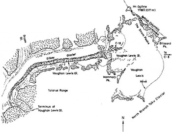
Fig. 3. The Lewis-Gilkey Glacier complex (Coyes, unpublished).

Fig. 4. Vaughan Lewis Ice fall (photograph by H. Rentsch).

Fig. 5. Set-up of the terrestrial photogrammetric observations.
Vaughan Lewis Glacier is categorized glaciothermally as being temperate and is considered to be a climatologically controlled, normal discharge-type glacier. Its source area lies at a mean altitude of 1680 m on the southern flank of Blizzard Range near Mount Ogilvie (Fig. 3). The ice flows westward off the nélvé plateau into Gilkey Trench, descending about 500 m in a spectacular ice cascade — the famous Vaughan Lewis Icefall (Fig. 4) — in a planar distance of only c. 800 m. At the base of the ice fall lies a series of extraordinary wave bulges, which are arcuate and convex down-glacier, and have an amplitude of up to 25 m and a wavelength of about 150 m. These wave bulges (also referred to as wave ogives) have been the subject of extensive studies (e.g. Reference FreersFreers, 1965; Reference Miller, Freers, Kittredge and HavasMiller and others, 1968; Coyes, unpublished; Kitteridge, unpublished). The investigations were carried out by participants in the Juneau Icefield Research Project (JIRP) and the Foundation for Glacier and Environmental Research (FGER); both programs were founded in 1946 and have been held annually since then.
Velocity measurements of the ice fall, however, have been rarely carried out, at the lower part of the ice fall which is not too difficult and dangerous for accessibility for terrestrial measurements. Vaughan Lewis Icefall is a typical example for the application of terrestrial photogrammetry.
The Dtm Of Vaughan Lewis Icefall
The primary data for the DTM were recorded from terrestrial photogrammetric stereo models from 15 August 1982. All measurements refer to a local coordinate system, defined by geodetic control points and camera positions (Fig. 5). For the photogrammetric evaluation, the analytical plotter ZEISS PLANICOMP C100 at the Chair of Photogrammetry of the Technical University Munich, has been made available.

Fig. 6. Shaded relief in orthogonal projection superimposed with contour lines and ice-movement vectors.
Along 5 m contour lines, 11 500 points have been recorded. In addition, 280 points along the boundary between the ice-covered surface and the surrounding bedrock were measured and introduced as break-line information. From these data, a regular grid DTM was interpolated using the program package HIFI-88. With regard to the distribution of the primary DTM data, a grid width of 20 m was selected. The generated DTM shows an r.m.s. of 2.1 m compared to the actual measurements; this is caused by the surface approximation with the grid elements and the smoothing effect of the bilinear interpolation, especially within the areas of fractured ice. Besides the essential advantages concerning data processing and storage, the regular grid DTM was necessary as a basic data structure for the DTM visualization.
Glacier Flow And Flow Velocity Of Vaughan Lewis Icefall
For the measurement of the surface-flow velocity of Vaughan Lewis Icefall, the glacier was repeatedly surveyed by terrestrial photogrammetry between 29 July 1982 and 19 August 1982. It was decided to measure about 240 single points for the velocity determination. They refer to morphological features of the ice fall which could be recognized on the images taken on different days. Their movements in time are a measure of the spatial velocities of these points. The standard deviations of the vectors from double measurements are 0.1 m in length and 4−in azimuth.
Figure 6 shows a plan view of the vector field of point velocities superimposed on the contour lines, and a digitally shaded relief model. The velocity of the ice increases to a maximum amount of 5.70 m d−1 at the narrowest gap between the bedrock banks on both sides. Where the slope flattens, the velocity decreases to 1 m d−1, and to 0.4 m d−1. Thus, the average velocity amounts to about 150 m year−1 at the foot of the ice fall, where the wave ogives occur. Remarkably, this annual surface velocity matches the average wave length of the ogives, a fact, which had been already observed by Reference HaefeliHaefeli (1951) on other glaciers. Thus, the velocity measurements help to explain some phenomena of the ice surface. The discussion of the glaciological phenomena encountered during the investigation of the ice fall is, however, beyond the scope of this paper.
Better Visualization By Means Of Digital Image Processing
From the DTM, further products can be derived by the use of digital image-processing techniques (Reference EbnerEbner, 1987; Reference Hanson and QuamHanson and Quam, 1988):
Colour-coded representations of height, slope, aspect, and height-difference information.
Shaded relief models in orthoprojection (also superimposed with terrain-cover information or contour lines).
Perspective views.
Stereo perspectives and videos.
In the following, the generation of some of these products is explained and illustrated by examples.
In a shaded relief, each elevation of the DTM is given a grey value (normally with a resolution of 8 bits), which in the simplest case is proportional to the cosine of the angle between the surface normal and the direction towards an artificial illumination source (Reference Stefanovic and SijmonsStefanovic and Sijmons, 1984). This light source is placed in the north-west, as it is common practice in cartography. For this purpose, the original 20 m by 20 m basic grid was densified to a 5 m by 5 m grid using the HIFI-88 program package. A shaded relief is very useful for the visual inspection of the DTM, since it is very sensitive to small height changes.
To visualize the shaded relief on a modern high-resolution graphics monitor with 1024 × 1024 pixels (picture elements), a further densification down to a mesh size of 2.5 m by 2.5 m is needed. This is done by using a bilinear interpolation. Then the terrain cover can be superimposed on to the shaded relief to obtain a synthetic terrain representation. The digitized terrain cover borders are vector-raster transformed and registered in a shaded relief. The colour or grey value of each cover type (rock, ice, snow, water, and moraine in the case of Vaughan Lewis Icefall) can be selected interactively on the monitor or taken from digitized photographs or satellite data (e.g. LANDSAT or SPOT). Thus, for each pixel, three-colour values (red, green, and blue) or one grey value are generated. The multiplication of these values with the grey value of the shaded relief yields the desired result (Fig. 7).
The procedure described here is the one used to merge raster data into a geographical information system (GIS) for the superimposition of vector data (Reference GöpfertGöpfert, 1987). Thus, all the GIS tools are readily available for further terrain analysis.
Another possibility is the derivation of inclination maps from the height data. The different inclinations can be grouped into different classes and displayed, one colour per class.
The products described so far can be compiled into cartographic maps. As such, they are scale-independent and can be updated or combined efficiently with thematic information by digital means.
A perspective representation of the relief offers further help for interpretation. After selecting a suitable viewpoint, the intersection between the ray of sight for each pixel of the new projection plane and the DTM is computed. The color or grey value of the shaded relief at the intersection point is assigned to the corresponding new pixel (method of ray tracing; Reference Thiemann, Fischer, Haschek, Kneidl, Hausmann, Hopgood and StrasserThiemann and others, 1989; Fig. 8).
Two perspectives with slightly different perspective centres (c. 5°in azimuth) form a pair of stereo photographs and can thus be viewed in three dimensions.
If the perspective centre is moved continuously in space and perspectives are calculated with small time intervals, the frames can be recorded on video tape. Displaying this video, one has the impression of flying across the terrain, and able to view the glacier from all sides.

Fig. 7. Shaded relief in orthogonal projection superimposed with terrain cover.

Fig. 8. Perspective view of the ice fall.
These perspectives, stereo perspectives, and videos open up new ways of interpreting glacier phenomena, because synthetic views can be generated from arbitrary projection centers. Especially, for the explanation of the topography and the geomorphology, they offer considerable assistance.
Conclusions
Digital terrain modeling has become a highly technical and fully operational tool, which can be integrated into glaciology and geoscience for better efficiency. The application of DTM, in combination with digital image processing, aids not only considerably the interpretation of surface phenomena but also opens up the way for new digital cartographic products. Furthermore, it is the first step in the integration of raster products into a GIS, allowing, for example, simulations of ice movement or melting, taking into account different terrain covers.
Acknowledgements
The authors are indebted to Professor Dr H. Ebner, Institute of Photogrammetry, Technical University Munich, for making the facilities of his institute available, to The Foundation for Glacier and Environmental Research, University of Idaho, Moscow, Idaho, for supporting the field work which has been and will always be the basis of all glaciological work, and K. Eder, Institute of Photogrammetry, Technical University Munich, for his assistance in generating the DTM of Vaughan Lewis Icefall.


