


Introduction
The conspicuous drainage of over 3000 supraglacial lakes on the surface of Larsen B Ice Shelf in the days prior to its sudden, catastrophic break-up in 2002 led to the widespread view that meltwater-induced hydrofracture could be an important process leading to ice-shelf instability (Scambos and others, Reference Scambos, Hulbe and Fahnestock2003). An additional process of viscoelastic flexure in response to changing meltwater loads associated with the filling and draining of supraglacial lakes may also have contributed to the widespread fracture of Larsen B (Banwell and others, Reference Banwell, MacAyeal and Sergienko2013; Robel and Banwell, Reference Robel and Banwell2019). A modeling study showed that seasonal- and annual-scale meltwater load changes across the ice shelf prior to break up were sufficient to cause fracture-inducing stresses where the ice shelf was relatively thin (Banwell and MacAyeal, Reference Banwell and MacAyeal2015).
Satellite observations of the McMurdo Ice Shelf (McMIS), Antarctica between 1999 and 2018 showed that the filling and draining of supraglacial lakes occurred on annual time scales (Macdonald and others, Reference Macdonald2019). Satellite and field observations on the McMIS over the 2016/17 summer showed that surface lake water volume also varied on seasonal to diurnal time scales, and that the lake volume changes over seasonal time scales were sufficient to induce ice-shelf flexure with resultant stresses that were sufficient to induce fracture (Banwell and others, Reference Banwell, Willis, Macdonald, Goodsell and MacAyeal2019).
As a result of a field observation study on the McMIS, conducted in austral summer of 2016/17 (Banwell and others, Reference Banwell, Willis, Macdonald, Goodsell and MacAyeal2019), filling and draining of supraglacial lakes were observed not only on the seasonal and annual time scales (see also Macdonald and others, Reference Macdonald2019), but also on the diurnal time scale. The possible causes of diurnal time-scale meltwater-depth fluctuations and their consequences in terms of ice-shelf flexure (and possible fracture) constitutes the subject of our study.
Here, we focus on the causes and consequences of the lake filling and draining that we have observed over diurnal time scales on the McMIS. We investigate two mechanisms that could cause meltwater depth to fluctuate at these time scales. The first is a mechanism that can only operate on ice shelves that float in ocean regions where there is a significant tide. Ocean tides in coastal regions can feature tidal range and amplitude variation with spatial scales in the 10s of kilometer range (e.g. Henderschott, Reference Henderschott1980; MacAyeal, Reference MacAyeal1984). An example would be where there is tidal resonance in an enclosed bay. For a floating ice shelf, variation of the tidal amplitude in such a bay would induce a fluctuating component in the gradient of the ice shelf's upper surface over the tidal period. This is depicted schematically in Figure 1, where the tidal elevation of the ocean/ice-shelf system, T, is depicted with a gradient that tilts the surface of the ice shelf containing supraglacial meltwater.
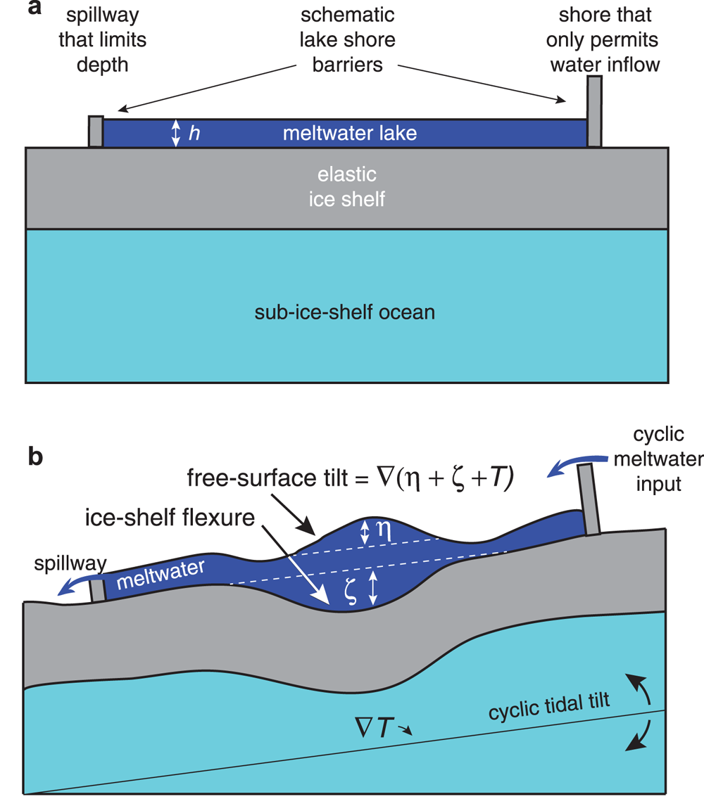
Fig. 1. Three-layered system used to model the movement of meltwater and associated ice-shelf flexure. (a) Depiction of a surface meltwater lake undisturbed by time-dependent inflows, outflows and the tilt of the ocean in which the ice shelf floats due to the ocean tides. The depth of the undisturbed meltwater lake, h, is assumed to be spatially uniform, the ice-shelf thickness is assumed constant, and elastic flexure of the ice shelf in response to the undisturbed is disregarded in the diagram for simplicity. Meltwater inflow from surrounding catchment areas is permitted (as shown for the boundary on the right in the diagram), but meltwater addition to the lake is assumed not to change the lake's horizontal extent. At one specific part of the boundary (the one on the left in the diagram), the boundary acts as a spillway to limit the depth of the lake at that location. (b) Depiction of the disturbed meltwater lake system in which meltwater depth is perturbed from its state of rest, h, by a free-surface perturbation η and a water/ice-shelf interface perturbation ζ associated with ice-shelf flexure in response to the movement of meltwater loads. The variables η and ζ combine with spatially variable tide elevation in the ocean below the ice shelf, T, to determine the slope of the meltwater's free surface. This slope, $\nabla \lpar \eta + \zeta + T \rpar$ , determines the direction and magnitude of water flow in the lake. In the case where meltwater-inflow cycling is examined as the cause of diurnal meltwater-depth variations, tidal tilt is assumed zero and a cyclic meltwater input is applied as a boundary condition along with a spillway-boundary condition that restores the mean depth perturbation to zero.
The second mechanism for diurnal time-scale meltwater-depth cycles is the diurnal variation of meltwater input into the lake driven by the daily melting cycle in the catchment area of the lake. If the lake is considered to be an open system, where water draining in from a catchment area can drain out either through a spillway (e.g. through an outlet stream system, possibly leading to other lakes downstream Kingslake and others, Reference Kingslake, Ng and Sole2015) or a moulin that has restricted flow, then diurnal depth fluctuations will occur if the drainage cannot match the input during parts of the day when input is enhanced. This is also depicted in Figure 1 by the two schematic barriers that constitute boundaries of the supraglacial lake. One schematic boundary, which we refer to as a ‘spillway’, is permeable to inflow only, and represents the lake shoreline where supraglacial streams enter from higher elevation areas. The other schematic boundary is permeable only to outflow when the depth at the shoreline exceeds a certain level.
The goal of the present study is to evaluate the importance of both tidal-tilt-driven and meltwater-input-driven fluctuations within supraglacial ice-shelf meltwater systems in general, and in the context of our McMIS field observations in particular. In our evaluation of tidal-tilt effects on meltwater, our focus will be on interior ice-shelf regions several kilometers away from grounding lines, where the significance of tidal tilt remains undetermined. For effects near grounding lines, we refer to Wild and others (Reference Wild, Marsh and Rack2018) (e.g. see their Fig. 5). In addition, we seek to determine circumstances where such fluctuations could have a bearing on ice-shelf stability. As we shall show below, both causes of ice-shelf water-level fluctuations are plausible, and the relative importance of one over the other depends on regional details of the ocean tide and the local hydraulic characteristics of the water bodies.
Field site and observations
This study is motivated by observations of decimeter-scale diurnal meltwater-depth fluctuations in a meltwater lake on the McMIS during the 2015/16 austral summer melt season. The region of the McMIS containing shallow (≤2 m deep) supraglacial lakes and streams is shown in Figure 2. The specific lake where diurnal meltwater-depth variations were observed is informally called Rift Tip Lake (Banwell and others, Reference Banwell, Willis, Macdonald, Goodsell and MacAyeal2019), because it formed in a minor depression of the ice-shelf surface in the vicinity of an ice-shelf rift terminus that had existed unchanged prior to our field program for about a decade, but which propagated in March 2016 (Banwell and others, Reference Banwell, Willis, Macdonald, Goodsell and MacAyeal2017). The ice shelf around Rift Tip Lake is partially covered by terrigenous and marine-sourced debris, lowering its surface albedo (Fig. 2, Glasser and others, Reference Glasser, Goodsell, Copland and Lawson2006). This debris, and a prevailing down-slope wind regime, means that the McMIS is one of the most southerly ice shelves to exhibit substantial surface melting (Kingslake and others, Reference Kingslake, Ely, Das and Bell2017).

Fig. 2. Rift Tip Lake and surrounding meltwater drainage features on McMurdo Ice Shelf, Antarctica. (a) Google Earth imagery (30 December 2016). (b) Interpreted supraglacial features connected to Rift Tip Lake. The lake is indicated by a blue-filled oval shape, and is roughly 600 m by 300 m in size. Surface streams connected with the lake are indicated by black lines. Drainage paths from the region drained by the streams to the ice front are indicated by blue arrows. Approximate location of continuous, static GPS survey benchmarks are denoted by stars and labeled 1, 2 and 3. (c) Satellite image of Rift Tip Lake (WorldView-2 image, 5 January 2013, provided by the Polar Geospatial Center, Imagery Ⓒ 2013 DigitalGlobe, Inc.).
We deployed two water-depth pressure sensors in Rift Tip Lake (approximately at its center, as best as we could estimate) for a 31-d period in December and January of 2015/16 as part of a larger study to understand the impact of surface melting and ponding on ice-shelf stability (Banwell and others, Reference Banwell, MacAyeal and Sergienko2013, Reference Banwell, Willis, Macdonald, Goodsell and MacAyeal2019). The sensors (HOBO water-level loggers, 0–9 m range, manufactured by Onset) were installed against an aluminum pole firmly drilled into the ice shelf. One sensor was fixed to the pole at a point just above the ice surface; the other rested on the bottom of the lake and was allowed to slide down the pole as the lake bottom ablated. Taken together, the readings allow the calculation of lake water-level fluctuations as well as lake bottom ablation rates. Barometer measurements at a nearby automatic weather station (AWS, Pegasus North, operated by the University of Wisconsin Antarctic Meteorological Research Center) were used to remove atmospheric pressure effects from the derived depth measurements.
Incoming solar radiation and 2-m air temperature were recorded for part of the 31-d observation period (from 31 December onwards) at a site informally known as Artificial Basin, situated ~8 km to the south east of Rift Tip Lake (Fig. 2a). These variables were measured with a Kipp and Zonen CNR4 and Vaisala HMP155A respectively, and 30-s samples were logged every 10 min on a Campbell Scientific CR1000 data logger. Ice-shelf elevation was recorded at four sites surrounding Rift Tip Lake using Trimble NetR9 GPS receivers with Zephyr Geodetic antennas recording on a 15-s interval (further details of the GPS measurements and processing can be found in Banwell and others, Reference Banwell, Willis, Macdonald, Goodsell and MacAyeal2019).
Observational results
The 31-d water-depth time series taken from the bottom/sliding pressure sensor displays three effects: (1) long-period (multi-day) filling and draining of the lake; (2) ablation of the lake bottom; and (3) diurnal-period fluctuations (Fig. 3a). The time series observed by the fixed pressure sensor (not shown) showed similar diurnal fluctuations, but the series was intermittent because water levels occasionally dropped below the sensor level. There were 24 distinct diurnal cycles of water depth over the 31-d observation period, ranging in amplitude (defined heuristically to be the peaks relative to the previous and following low-depth troughs) from ~35 cm to just barely 1 cm. Both a pressure sensor and a time-lapse camera system recorded similar water-depth fluctuations in Rift Tip Lake in the subsequent melt season (2016/17) (Banwell and others, Reference Banwell, Willis, Macdonald, Goodsell and MacAyeal2019).

Fig. 3. (a) Water-depth fluctuations; (b) GPS vertical elevation (relative to 60-d time average of GPS observations at the site); (c) insolation (theoretical clear-sky limit computed using the local solar zenith angle, a 1366 W m−2 solar constant and a 95% clear-sky transmission coefficient, and observed using a four-component radiometer; and (d) measured 2-m air temperature at Rift Tip Lake on the McMurdo Ice Shelf. The AWS measurements at Artificial Basin site (see Fig. 2a for location) did not cover the complete period of time the water-depth and GPS observations were made.
To investigate the possible causes of the diurnal cycles in water depth, we compared them to similar cycles in (1) vertical elevation of the ice shelf measured by the GPS receivers; (2) insolation (both theoretical, computed for clear-sky conditions, and observed); and (3) 2-m air temperature (Figs 3b–d). All variables have a strong diurnal cycle, but no particular one appears to align consistently in phase better than the others.
To investigate the data further, we focus on the co-variation of the four variables over the 4-d period when depth variations were most pronounced and when the sky was clear of clouds, as indicated by the incoming shortwave radiation, notably 13–17 January 2016 (Fig. 4). Except for incoming shortwave radiation and 2-m air temperature, which vary closely in phase, all variables are out of phase with each other (Fig. 4). We performed a trial and error fit by eye to determine what phase shifts are required to align the cycles in the time series. We determined that the ice-shelf elevation series would have to be advanced by 16.5 h (or lagged by 7.5 h) to align this surrogate for the ocean tide with the lake-depth maxima, and that the insolation/air temperature series would have to be advanced by 5.5 h (or lagged by 18.5 h) to align these proxies for meltwater inputs with the lake-depth maxima (Fig. 4c).

Fig. 4. (a) Normalized observed variables: water depth η, ice-shelf elevation (ζ + T), incoming shortwave radiation, and 2-m air temperature over the 4-d period (13–17 January 2016) when water-depth fluctuations were most pronounced and where insolation was principally clear sky (Fig. 3). A legend signifying pairing of variables and line colors is provided above panel (a). Downward spikes in incoming shortwave radiation are caused by the AWS mast shadowing the radiometer. Normalization is accomplished by dividing the observed signal by the difference between maximum and minimum values over the 4-d period. Ice-shelf elevation was smoothed by a 1 h running mean of the GPS data. The water-depth time series has additionally had its mean and linear trend removed. (b) Each day's variation is plotted as a function of that day's time-of-day (UTC) to assess consistency of timing relationships and to judge time lags. (c) The normalized series of ice-shelf elevation must be shifted forward in time by 16.5 h, and the normalized shortwave input by 5.5 h, respectively, to align peak-to-peak with the meltwater-depth observation.
The diurnal depth fluctuations could not easily be explained in terms of any one of the prospective forcing variables (tide, insolation and air temperature). This motivated us to conduct the more in-depth analysis presented below. What follows is our effort to develop a simple dynamical framework for understanding diurnal fluctuations of meltwater depth in lakes and streams on ice shelves. Ultimately, we show via a pair of idealized numerical simulations of the Rift Tip Lake data that diurnal incoming shortwave radiation variations provide the most likely explanation of the observed meltwater-depth fluctuations. We also show that small, but non-negligible, fluctuations in water depth are caused by the tilt of the ice shelf associated with the underlying ocean tide.
A simplified model of meltwater lakes on ice shelves
To explore the phenomenology of diurnal depth fluctuations in ice-shelf surface lakes, whether caused by tidal tilt or by meltwater input cycles, we create a simple model of surface meltwater movement and ice-shelf flexure. This model will be used to conduct two numerical simulations designed to test each of the possible two causes of the diurnal water-level fluctuations to see which agrees best with observation. The model also serves to illustrate the essential difference between surface hydrology on grounded ice sheets and floating ice shelves.
A schematic diagram of the supraglacial meltwater system, as it is idealized in this study, is provided in Figure 1. The tilt of the free surface of the meltwater lake or stream is determined by the gradient of three variables: η the perturbation to the mean (presumed to be flat, when tide and flexure are eliminated) depth of the meltwater, ζ the perturbation to the ice-shelf surface due to elastic flexure in response to meltwater load and buoyancy, and T the perturbation of the ocean surface due to the large-scale ocean tide. The free-surface tilt, $\nabla \lpar \eta + \zeta + T \rpar$ , determines the pressure gradient in the meltwater layer, where $\nabla = \lpar {\partial }/{\partial x}\rpar {\bf e}_{x} + \lpar {\partial }/{\partial y}\rpar {\bf e}_{y}$
 is the horizontal gradient operator and x and y are horizontal Cartesian coordinates. All variables are functions of time, t, and are listed along with equations relating them in Appendix A. We assume that the mean, unperturbed depth of the meltwater is constant at 1 m for simplicity. This idealization is based on observations of meltwater lakes on other ice shelves (e.g. Banwell and others, Reference Banwell2014) and in our field area. Appendix B presents an initial overview of sensitivity of lake-depth fluctuations to various assumptions and parameters.
A key simplifying assumption of the model is that we disregard inertial forces. This removes the wave-like response of the meltwater system that governs η(x, y, t) over time scales that are short compared with the time scale ${L}/{\sqrt {g h}}$ needed for a shallow-water gravity wave to traverse the meltwater feature (the lake and the streams that feed it from the lake's catchment area), where L is the length scale, g = 9.81 m s−2 is the acceleration of gravity, and $\sqrt {gh}$
 is the phase speed of a shallow-water gravity wave in water of depth h. Typically the time scale associated with ${L}/{\sqrt {g h}}$
 is on the order of seconds to minutes, whereas we are interested in phenomena that vary with the tide (12–24 h time scale). The effect of this simplifying assumption is to produce two end-member force balance regimes, one where the water level is maintained flat quasistatistically, and one that is dominated by friction. When friction effects are small (i.e. the ice-shelf surface presents little resistance to meltwater flow in the form of roughness), the pressure gradient is not balanced by any force (since inertia is disregarded). This implies that it is identically zero, $\rho _{\rm w} g \nabla \lpar \eta + \zeta + T \rpar = 0$
 , thereby necessitating $\lpar \eta + \zeta + T \rpar = {\rm constant}$
 . In this case, the meltwater feature and ocean tide are related in the same way as coffee in a coffee cup that is slowly being tilted from side to side. As the coffee cup slowly tilts, the coffee it holds maintains a flat surface.
The other end-member is where pressure gradients are balanced by friction caused by meltwater flow over a rough ice-shelf surface. To parameterize friction, we use a linear treatment of the Manning formula (Gleason and others, Reference Gleason2016; Smith and others, Reference Smith2017) to derive (see Appendix A) the following diffusion equation for how meltwater depth changes in response to pressure gradient,

where $\tau \in \lsqb 100\, {\rm s}\comma\; 10000\, {\rm s}\rsqb$ is a frictional-damping time scale obtained from linearizing the Manning formula. This diffusion equation results from combining the momentum-balance equation (balancing friction with pressure gradient) and the mass continuity equation. When τ is very large, the friction term is small, implying that the pressure gradient is zero. When τ is very small, the movement of water mimics a diffusion process with a diffusivity of g hτ. We describe sensitivity to assumptions in Appendix B.
The variable ζ is determined using a 4th-order elliptic partial differential equation to represent elastic flexure in response to water-load perturbations ρ wgη and buoyant forces acting on the perturbed ice-shelf flotation level ρ swgζ. Here, ρ w is the density of fresh meltwater and ρ sw is the density of the ocean water in which the ice shelf floats. The assumptions made to simplify the elastic flexure of the ice shelf are that (1) the thin-plate approximation applies, and (2) the flexure is sufficiently slow that the inertia of the ice shelf's vertical movement is zero (this is also the assumption for the shallow-water momentum balance). The elliptic partial differential equation is 4th order in space and has no time dependence; hence, it is a diagnostic equation that can be solved in concert with the solution for the time-dependent functions η and T. The tide T is determined externally as the forcing of the problem (in the case of sympathetic tides) and is described in the next section. Further details describing η, ζ and T are provided in Appendix A.
Numerical experiment design
Two numerical experiments are done to explore the limiting behaviors of surface meltwater lakes on ice shelves. Because of the paucity of observations, and the lack of constraints on model parameters and assumptions, two simulations are considered sufficient as an exploratory illustration, one to investigate tidal tilt and one to examine cyclic meltwater input. The key difference between these two experiments is the treatment of meltwater system geometry and boundary conditions. For the tidal-tilt experiment, we assume that the meltwater features are closed, with no flux across their boundaries. We further assume that the boundaries remain fixed through the tidal cycle, even though in reality they may extend and shrink. Finally, we disregard meltwater input from the upstream catchment areas, because including input would mix the two forms of forcing we are trying to differentiate.
For the meltwater input experiment, we assume tidal tilts are zero but allow the boundaries of the meltwater features to be open. This permits meltwater input from upstream catchment areas that do not contain standing water. Because the relationship between meteorological conditions and the observed meltwater-depth fluctuations are complex (as suggested by Figs 3, 4), the meltwater input across the boundaries is simplified by applying a diurnal pulse of meltwater as a boundary condition on the meltwater system, which is balanced by a spillway-type boundary condition at the lake's downstream outlet (Fig. 5). The spillway-type boundary condition allows water to flow out of the domain (into the ocean) whenever the meltwater surface is above the level it would be if there were no inputs to the system.

Fig. 5. (a) Idealized meltwater-flow topology and numerical model domain used in exploratory modeling to assess the cause and effects of surface meltwater-level fluctuations in the lake. (b) Close up of Rift Tip Lake, as idealized in the model. (c) Simplified geometry for the meltwater-input simulation.
At boundaries where meltwater flows into the lake, we specify:

and, at the spillway boundary, we have:

where A is an amplitude, α ≈ 10 is a spillway impedance, and ${\bf n}$ is the outward pointing normal vector to the contour of the boundary. The treatment of the spillway is such as to maintain the lake level at η = 0 when there is no input. When there is an input, the lake level oscillates sinusoidally with a frequency σ in time t at the input, but remains positive definite. The value of the spillway impedance α was chosen arbitrarily so as to avoid a situation where the time average of η becomes greater than about 10 cm. Unlike the tidal-tilt simulation, where the time mean value of η is zero, the meltwater input simulation attains a positive value of η over all of the cycle, because meltwater is always moving from the input boundary to the spillway boundary.
As shown in Figure 5, we adopt an idealized geometry. Rift Tip Lake is taken to be an elliptical basin, approximately 600 m (E/W) by 300 m (N/S), at the western end of an approximately 2 km long, E/W trending rift that has evolved to become a channel-like feature, ~10 m wide, that can contain and convey meltwater. The rift and the lake basin, whether dry or filled, existed in a similar form from about 2002 to March 2016. In March 2016, the rift propagated to the west, however the lake basin, formerly at the rift tip, continued to fill in 2016/17. The drainage system of McMIS in the vicinity of Rift Tip Lake trends from the south toward the ice front and is represented by a series of confused meltwater streams that intersect the southern side of the lake. We represent this drainage system by an idealized array of streams, some of which include small pools and lakes along their course, that emanate from the lake's southern boundary and extend approximately 12 km across a region covering approximately 4 × 10⁷ m2 (Fig. 5).
For both experiments, we assume a frictional damping timescale of τ = 1000 s, which is consistent with a Manning roughness coefficient of ~0.1 m s1/3. The value of the Manning coefficient used in this study is an order of magnitude larger than the values typically used for supraglacial streams in other studies (Gleason and others, Reference Gleason2016; Smith and others, Reference Smith2017). In our study, the larger value is chosen to allow typical water flow speeds in our simulations to be on the order of several cm s−1 in the meltwater channel feeding the lake. This flow speed is consistent with what was seen casually in the field (we were not able to make precise measurements). A possible physical explanation for using the larger value is the fact that the much reduced surface slopes typically found on thin ice shelves like the McMIS prevent the flow in supraglacial streams from eroding roughness that would be missing from streams on steeper ice-sheet surfaces such as in Greenland. The mean water depth was taken to be 1 m. In practice, the variation of gτh = 9800 m2 s−1 represents the critical diffusivity-like parameter that governs water movement; so variations in τ and h are not independent.
To force the tidal-tilt experiment, we employ a simple oscillating tilt that is homogeneous over the basin and varies sinusoidally in time. This simplification is consistent with the assumption that the ocean tide is propagating as a large-scale Kelvin wave (Henderschott, Reference Henderschott1980; MacAyeal, Reference MacAyeal1984; Padman and others, Reference Padman, Siefgried and Fricker2018). The periodicity of the tidal tilt is taken to be that of tidal constituent K1, with a period of 23.934 h. We assumed a tidal tilt of 0.5 cm km−1 in the N-S direction which corresponds to a tidal amplitude variation perpendicular to the coast in the vicinity of Rift Tip Lake. This assumed tidal-tilt magnitude is justified in Appendix C. With this forcing, the tidal elevation of Rift Tip Lake is lower than the tidal elevation of the distal, southern ends of the meltwater channels in Figure 5 by about 6 cm when the tide in McMurdo Sound is high. The elevation at the lake is likewise 6 cm higher than the distal ends of the streams at low tide. This difference in tidal elevation is consistent with what we assume to be an off-shore decay of tidal amplitude that is consistent with Kelvin wave propagation (Henderschott, Reference Henderschott1980). The amplitude of the sinusoidally varying tidal tilt is therefore 5 × 10⁻⁷ for this experiment. Direct confirmation of this degree of tidal tilt is discussed in Appendix C, where analysis of GPS data from two sites shows a ~1.4 cm tidal elevation difference over the span of ~3 km.
To force the meltwater-input experiment, we assumed an average daily meltwater flux into the boundary of the model domain of F = 2 × 10⁵ m3 d−1, which is roughly consistent with estimates made in the field (we did not precisely measure meltwater flux). This flux corresponds to about 0.25 cm d−1 of melting over the ~ 4 × 10⁷ m2 area of the ice shelf that is drained by the stream network to the south of Rift Tip Lake. The boundary condition specified at the input boundary (Fig. 5c) is

where W = 10 m is the width of the inlet boundary, and where σ d = 2π/24 h−1 is the diurnal solar frequency. This representation of the input flux is always positive definite. The input flow boundary never removes water from the system. The boundary condition at the spillway boundary (Fig. 5c) is as shown in Eqn (3) with the constant α = 10 m2 s−1. This choice of the spillway impedance parameter α is consistent with observations of 1–10 cm s−1 water flow in the ~10 m wide, ~1 m deep outlet channel draining Rift Tip Lake.
Simulation results
The results of the two simulations for tidal tilt and meltwater input cycling are shown in Figures 6 and 7, respectively. The fields shown in Figures 6 and 7 represent the amplitude of the sinusoidal cycles in η, ζ and the maximum stress magnitude due to flexure in the ice at either the upper or lower surface (using the von Mises stress T vm as the measure of magnitude).
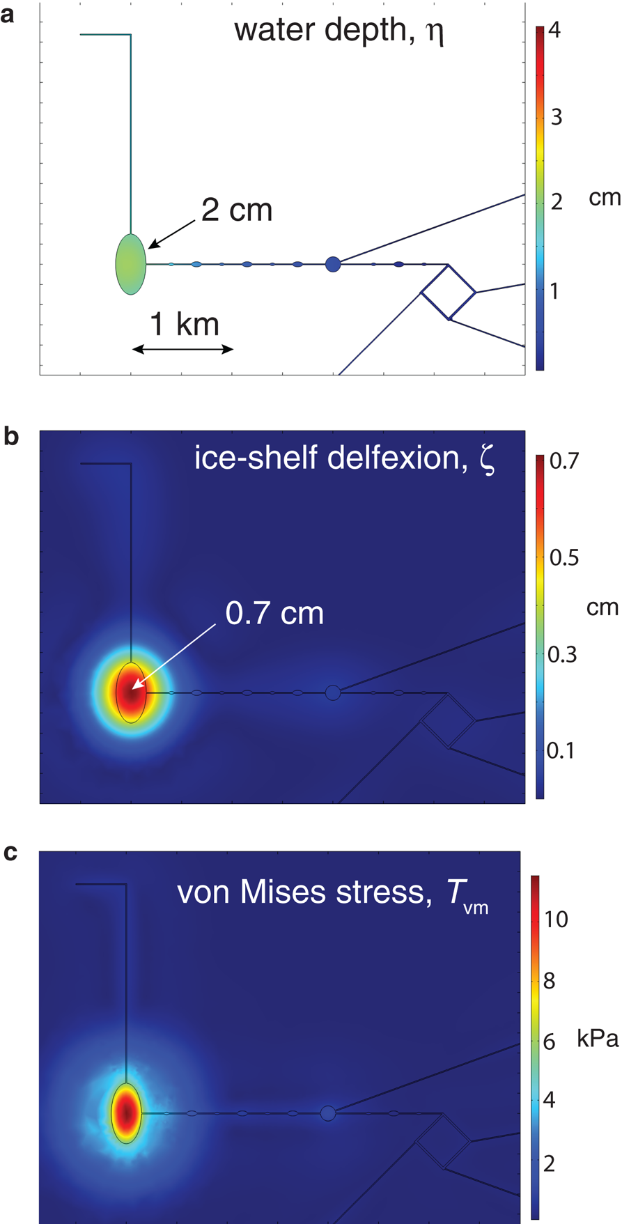
Fig. 6. Tidal-tilt cycle simulation results: (a) amplitude of lake-depth variation η, (b) amplitude of ice-shelf deflexion ζ, and (c) von Mises stress T vm. In panels (a) and (b), amplitudes at specific locations are annotated by arrows and centimeter values.

Fig. 7. Meltwater-input cycle simulation results: (a) amplitude of lake depth variation η, (b) amplitude of ice-shelf deflexion ζ, and (c) von Mises stress T vm is shown. In panels (a) and (b), amplitudes at specific locations are annotated by arrows and centimeter values.
The impact of the meltwater-depth oscillations on the ice shelf is assessed by the positive-definite quantity that measures stress magnitude commonly used in fracture mechanics: the von Mises stress T vm defined by

where the various terms on the right-hand side are xx, yy and xy components of the deviatoric stress tensor caused by bending. Note that the stresses use the variable T ij with subscripts, whereas T appearing without subscripts refers to the tide elevation. As a result of the thin-elastic-plate approximation, the flexure stresses vary linearly with distance through the ice shelf, and are always zero at the neutral plane of the ice shelf, which in our study is assumed to be half way between the upper and lower surface of the ice shelf. For the field area of Rift Tip Lake where the ice shelf is 30 m thick, the neutral plane is assumed to be at 15 m depth. We do not account for the complexities of elasticity variation with depth due to temperature or other variations associated with natural ice conditions. We display the value of T vm obtained at the upper and lower surface of the ice shelf, as this is where it is both maximum and where fractures introduced by flexure stresses likely originate.
To compare the two experiments, we choose to highlight the variables along the cross-sections shown in Figures 6 and 7 which extend from north of the lake to the south beyond the various junctions of the meltwater streams that feed the lake. The variables on these cross-sections are shown in Figure 8.

Fig. 8. Results for (a) tidal tilt and (b) meltwater input along a 4-km section extending from 500 m North of Rift Tip Lake toward the South. All lines represent maximum amplitudes achieved through the cycles for the respective variables. Tidal-tilt effects are small in amplitude and lag high tide by less than an hour, and are probably not able to explain the water-depth observations (Fig. 3a). Meltwater input cycling effects (based on the assumption of a net melting rate of 25 cm d−1 over a 4 × 10⁷ m2 catchment area that is sinusoidal and locked in phase with the local solar time) have an amplitude that is consistent with the water-depth observations (Fig. 3a).
For the tidal-tilt experiment (Fig. 8a), the amplitude of the variables are shown (each variable, η, ζ and T vm is assumed to vary sinusoidaly with time with the frequency of the leading diurnal tidal constituent (K1)). This means that the range of variation for η and ζ will be twice the amplitudes shown in the figure, as η and ζ will both be negative for half of the tidal cycle. The T vm is a positive-definite quantity, so it will vary at twice the tidal frequency; however, the individual stress components T ij will vary with both signs as a proper sinusoid at the tidal frequency. The range of water-depth variation at the center of the lake is about 4 cm (2 × amplitude shown in Fig. 8a). Although not shown, this maximum water depth (~2 cm above mean) occurs approximately 1 h after the time of high tide when the ice shelf is tilted so as to allow meltwater to run North into the lake from the stream network on the South. The maximum von Mises stress is about 12 kPa, which is well below what is thought to be the fracture criterion for ice (e.g. as cited in Albrecht and Levermann, Reference Albrecht and Levermann2012; Banwell and others, Reference Banwell, MacAyeal and Sergienko2013; MacAyeal and Sergienko, Reference MacAyeal and Sergienko2013; Banwell and MacAyeal, Reference Banwell and MacAyeal2015). Figure 8a does not show the amplitude of water depth at the distal ends of the streams south of Rift Tip Lake. Depth variation amplitude in the distal ends are 4 cm in the simulations, and the distal ends would be likely places to obtain more observations in the future to further evaluate the possibility of tidal-tilt-driven water-level oscillations.
For the meltwater input cycle experiment (Fig. 8b), the maximum value of the variables are shown, because all variables are positive definite and vary from 0 to the values shown in the figure over the cycle simulated. The range is thus shown directly by the figure. Water depth in the center of the lake reaches a maximum of ~22 cm above 0 (implying a sinusoidal amplitude of ~11 cm). This range of water-depth variation is consistent with what is observed (Fig. 3), however, this consistency depends entirely on the value used for the flux F specified at the input boundary. The varying water depth (not shown) displays a time lag relative to the phase of the meltwater input at the influx boundary. This time lag is about 1.5 h, meaning that high water in the lake occurs about 1.5 h after the maximum inflow at the influx boundary. This lag is determined by the time it takes for meltwater to flow through the streams leading to Rift Tip Lake, and thus depends on the Manning roughness coefficient we have chosen (based on very rough estimates of water flow speed in the field). Flexure stresses in Rift Tip Lake were in excess of 120 kPa at the time of maximum water depth (Fig. 7c). This stress magnitude is on the order of what may initiate fracture in an ice shelf (Albrecht and Levermann, Reference Albrecht and Levermann2012; Banwell and others, Reference Banwell, MacAyeal and Sergienko2013), although we did not observe such fracture in the field.
Discussion and conclusion
The output from the two numerical experiments can be compared with our observations from Rift Tip Lake. We first discuss the output from the tidal-tilt experiment and then from the meltwater input experiment. For the tidal-tilt experiment, the maximum range of depth fluctuations in the lake was 4 cm (twice the amplitude shown in Fig. 8a). This is much smaller than the observed depth variations which exceed 35 cm on some days (Fig. 3a). In addition, the linearity of the tidal tilt Eqn (1) suggests that the amplitude of the tidal-tilt response should scale with the tide, most notably with the 14-dspring-neap tidal beat cycle that is evident in the GPS data (Fig. 3b). However, the observed depth fluctuations show intermittent amplitude variation that is unlike the trends in the daily tidal range. Finally, the experimental maximum depth occurs within an hour of the high tide which, according to our assumptions is the case for the McMIS (see Appendix C), is when maximum tidal tilt occurs. (We note, of course, that tidal conditions for real ice shelves may maximize tilt at other phases of the tide.) The observations at Rift Tip Lake do not display a near zero time lag between the tide and the maximum depth. Instead, they show the maximum depth occurs at slack tide, half way between low and high tide, or about 15.5 h behind high tide. These three inconsistencies between the experimental results and the observations lead us to reject the idea that tidal tilt is the principal cause of the observed diurnal variations in meltwater depth at Rift Tip Lake.
Although we reject tidal tilting as a mechanism for driving the decimeter scale meltwater-depth variations on the McMIS, we remark that this mechanism may have a stronger importance on other ice shelves where tides are larger and where meltwater lakes may be located within the tidal flexure zone bordering the ice-shelf grounding line. Lenaerts and others (Reference Lenaerts2017), for example, describe supraglacial and englacial meltwater bodies within the grounding zone where tidal tilts are large due to boundary conditions imposed by neighboring grounded ice. Our results suggest that, in grounding zones where there is significant surface meltwater, tidal flexure will be both greater in amplitude and more complex in pattern than what would be the case for dry ice-shelf grounding zones (e.g. Rosier and others, Reference Rosier2017; Wild and others, Reference Wild, Marsh and Rack2018). Local amplification of the tide in response to ocean geometry may also produce situations where tidal-tilt may become important in driving meltwater lake oscillations. The ice shelves along the eastern side of the Antarctic Peninsula, for example, experience a tidal range that approaches 6 m over length scales that are on the order of 104 m and less (depending on coastal amplification). This means that the surface of such ice shelves can exhibit tilts of up to 10−5 (1 cm over a distance of 1 km). Assuming the upper bound tilt of 1 cm over distances of 1 km, meltwater features on the Larsen B Ice Shelf which were 10's of km in extent (Glasser and Scambos, Reference Glasser and Scambos2008) could have experienced tides of 10's of cm in amplitude.
For the meltwater input experiment, the amplitude of lake-depth variation was on the order of decimeters (Fig. 8b), which is consistent with observations (Fig. 3a). In addition, there can be various time lags across the meltwater feature so that the time of maximum water depth can also vary. This time lag is determined by the frictional constant τ and by the volume of the lake basin relative to the other meltwater features, notably the stream system that delivers meltwater to the lake. Meltwater input experiments done to investigate this time lag and other parameter sensitivities (these other experiments are not shown) revealed that the model could produce a meltwater-depth peak at any time of day simply by adjusting the timing of inflow at the boundary. Thus it is mainly the consistency between amplitudes of simulated and observed depth variations at Rift Tip Lake that cause us to conclude that diurnal meltwater cycles catchment area are likely driving the observed lake-depth fluctuations. We note, however, that the observed response is complicated and intermittent (with amplitudes varying over time and over some of the observation period). Our model is therefore too simple to capture these features.
A full characterization of meltwater input cycles driven by diurnal melting and runoff remains for future work, when there is greater constraint provided by more comprehensive observation of melting conditions and runoff friction. The approach to simulating meltwater input in the present study is simplified, and excludes an explicit treatment of critical elements of the problem such as the geometry of streamflow leading to the lake and the size and runoff efficiency of the catchment areas that feed the streams. We also lack a good model for diurnal melting in the catchment area that accounts for the complexity of the McMIS's partial debris cover. The simplified, incomplete model we used in this study was, however, sufficient to allow us to favor meltwater input cycles over tidal-tilt cycles as the origin of the observed fluctuations at Rift Tip Lake. To develop the meltwater input model beyond the level achieved here, more detailed observations of melt phenomena on ice shelves are necessary.
Having concluded that meltwater input is more likely than tidal tilt to explain the observations at Rift Tip Lake on McMIS (but that tidal-tilt cycles may play a minor role as their effects are small), we now speculate on the wider significance of the phenomena described in this study. First, we see that meltwater-depth cycles are exaggerated by the fact that the ice-shelf flexes in response to the additional weight of the moving meltwater (Fig. 8). This is not the case for supraglacial meltwater systems on grounded ice sheets and glaciers. Second, meteorological conditions driving diurnal melt cycling and runoff characteristics determined by surface roughness will largely determine the diurnal fluctuations in meltwater levels across the surface of melting ice shelves. Third, in some special cases, however, perhaps when lakes are unusually large (thereby spanning a wide zone of tidal amplitude variation) and located in places where tidal tilts are high, sympathetic tides in the surface meltwater systems may be driven by tilts induced by the ocean tides. Such special cases may have existed in the Labrador Sea prior to Heinrich events (Arbic and others, Reference Arbic, Mitrovica, MacAyeal and Milne2008) and on the Larsen B ice shelf prior to its 2002 collapse (Scambos and others, Reference Scambos, Hulbe and Fahnestock2003). On the Larsen B, lake geometries (Glasser and Scambos, Reference Glasser and Scambos2008; Banwell and others, Reference Banwell2014) were significantly larger in horizontal scale than on the McMIS and the tidal amplitude in the Western Weddell Sea (Robertson and others, Reference Robertson, Padman and Egbert1985; Padman and others, Reference Padman, Erofeeva and Joughin2003b; King and others, Reference King2011; Mueller and others, Reference Mueller2012; Rosier and others, Reference Rosier, Green, Scourse and Winkelmann2014; Zaron, Reference Zaron2018) is large compared to that in the McMurdo Sound. Whether tidally-driven or meltwater-input-driven lake-depth variations were active on the Larsen B ice shelf prior to its demise shall remain unknown, as the question of lake-depth fluctuations on diurnal time scales was not previously asked, and now the ice shelf is no longer there.
Our most important conclusion is the realization that lake-depth fluctuations driven by ocean tides and diurnal meltwater flux cycles can be associated with significant (10's of kPa) flexure stresses, particularly in the case where the ice shelf is thin. This amplifies the work of Banwell and MacAyeal (Reference Banwell and MacAyeal2015) and Banwell and others (Reference Banwell, Willis, Macdonald, Goodsell and MacAyeal2019) who investigated the effects of longer-term lake-depth fluctuations associated with seasonal filling and draining. These flexure stresses may be of a magnitude, in our study, to induce ice-shelf fracture. Numerical experiments (not shown) with larger ice-shelf thicknesses, e.g. with H = 200 m, as was roughly the ice thickness of Larsen B Ice Shelf before its collapse, show that the greater rigidity of a thick ice shelf causes the flexure, and flexure stresses associated with decimeter-scale meltwater-depth fluctuations, to become negligible. Ice-shelf thinning combined with increases in surface melting thus represents an evolutionary pathway for a thick, dry ice shelf to become less stable. This represents one more element of destabilization that must be thought about as ice shelves evolve in a future warming climate.
Acknowledgments
Data are freely available and archived at the United States Antarctic Program Data Center (USAP-DC), the National Snow and Ice Data Center (NSIDC) and the Antarctic Meteorology Research Center (AMRC) of the University of Wisconsin. This work was supported by US National Science Foundation (NSF) grants PLR-1443126 and PLR-1841467 awarded to the University of Chicago, NSF PLR-1841607 awarded to the University of Colorado at Boulder, and the UK NERC grant NE/T006234/1. ICW was supported by a CIRES Sabbatical Visiting Fellowship, AFB was supported by a Leverhulme Early Career Fellowship (ECF-2014-412) and a CIRES Post Doctoral Visiting Fellowship at the University of Colorado, and GJM acknowledges support from the NASA Earth & Space Sciences Fellowship (NNX15AN44H). GPS equipment and support was provided by UNAVCO. Geospatial support for this work was provided by the Polar Geospatial Center under NSF-OPP awards 1043681 and 1559691. Assistance in the field was generously provided by Brendan Hodge of UNAVCO, and Mike Cloutier of the Polar Geospatial Center. David Mayer at the University of Chicago (now at USGS) provided invaluable GIS support. The study has been significantly improved as a result of reviews bytwo anonymous referees, the Scientific Editor, M. Koutnik and the Associate Chief Editor, Ralf Greve.
APPENDIX A. Derivation of model equations
The shallow-water equations applicable to the surface meltwater layer are written


where η, ζ and T are the water-depth perturbation, the elastic ice-shelf deflexion and the ocean tide, respectively, where


and where ${\bar \cdot}$ denotes the long-term average operator, u and v are the x and y components of meltwater velocity ${\bf u}$
 (assumed independent of z, the vertical coordinate), g is the acceleration of gravity, and M is the Manning roughness coefficient taken to range from 0.01 to 0.15 s m1/3 (Smith and others, Reference Smith2017). In writing the above equations, we have chosen to disregard Coriolis forces to simplify the analysis here. This disregard is justified by the fact that the horizontal span of meltwater regimes on ice shelves is order 1–10 km in scale, and rotation effects are commonly disregarded in such small water bodies (Mortimer and Fee, Reference Mortimer and Fee1976).
Our first simplification is to linearize the equations by disregarding the ${\bf u} \cdot \nabla$ terms, replacing h with ${\bar h}$
 , and writing the friction in terms of a frictional timescale τ:

Taking h ~ 1 m and $\left \vert {\bf u} \right \vert \sim 0.01$ m s−1, we have

Equations (A1) and (A2) are now written,


We now operate on the first of the above equations with the operator

and use the second equation to replace the result of the operator acting on ${\bf q}$ in the right-hand side of the resulting equation to get:

We now non-dimensionalize the variables using scales L ~ 103 m for x and y, h o ~ 1 m for ${\bar h}$ , T o ~ 1 m for η, ζ and T, and $\sigma = \lpar {2 \pi }/{24}\rpar \, {\rm h}^{-1}$
 for ∂/∂t terms. The result, after a bit of algebra, is

where the variables are now scaled in dimensionless form. We now evaluate the two parameters appearing on the left-hand side of the above equation:

We thus disregard the acceleration term involving ∂2η/∂t 2 term on the left-hand side of the above equation while retaining the ∂η/∂t term, giving as the final simplified result:

where we have dropped the ${\bar \cdot}$ notation over h, and which is a diffusion-type equation for the variable η. This constitutes the derivation of Eqn (A14).
The equation governing ice-shelf flexure ζ(x, y, t) treats the ice shelf as a thin elastic plate lying above an infinite half-space ocean (MacAyeal and others, Reference MacAyeal, Sergienko and Banwell2015):

where ρ sw = 1028 kg m−3 is the density of seawater, ρ w = 1000 kg m−3 is the density of meltwater on top of the ice shelf, M xx, M xy and M yy are the bending moments which are related to the curvature of the flexure by the following expressions:


The variable H is the effective ice-shelf thickness (with regard to flexure) and is taken to be constant at 30 m which is consistent with what is observed near Rift Tip Lake (Rack and others, Reference Rack, Haas and Langhorne2013), E = 5 GPa is the Young's modulus for ice, and is taken to be in the middle of the observed range of variation for natural ice (1–10 GPa), and μ = 1/3 is the Poisson ratio for ice. Elastic parameters and ice-shelf thickness influence the resultant flexure in a manner that is captured by a single parameter $\cal F$ , the elastic rigidity:

which shows that the resistance to flexure increases with the cube of the ice thickness. This parameter is also involved in determining the horizontal length scale of ice-shelf flexure effects, and hence what size the surface meltwater lake must be to be significantly influenced by flexure, and vice versa.
APPENDIX B. Sensitivity of supraglacial meltwater response tidal tilt
Although our study concludes that tidal tilt was not the likely cause of diurnal meltwater-depth variations on the McMIS, our study did not rule out the possibility that tidal tilt could be a significant factor in driving surface meltwater oscillations in some circumstances (i.e. surface meltwater regimes with large horizontal scale in regions of high tidal amplitude variation). Even though tidal-tilt-driven meltwater phenomena may ultimately prove to be negligible, it is important that future investigation of its possible workings are appraised so as to avoid negative confirmation bias. We thus examine the response to tidal tilt in a more comprehensive manner in this appendix.
Equations (A14)–(A17) used in this study represent a highly simplified (linearized, simplified friction and boundary conditions) model of surface meltwater behavior in the ice-shelf/ocean system, and depends on three non-dimensional parameters:


where Δρ = ρ sw − ρ w ~ 28 kg m−3 is the density difference between salty seawater and meltwater. The model equations are now examined in light of the possible variation of the above parameters to determine representative behaviors that may exist under the great variety of conditions expected on an ice shelf.
Regime I. Friction-free, rigid ice shelf
If τ ≫ 103 s and L is appropriately small (<10 km), we expect κ > 102, and if we also consider the ice-shelf to be sufficiently stiff, with ${\cal F} \gg 1$ (e.g. by requiring H to be 100 m or greater), the governing equations (in dimensional form) reduce to


The first of the above equations is twice integrable to yield,

where $\cal A$ is the region of each closed, internally connected meltwater system. The integral in the above solution is the constant of integration (the linear term depending on x and y coming from the first integral of Eqn B10 must be zero to satisfy zero gradient, and thus zero meltwater flux, at the boundaries of $\cal A$
 denoted by $\delta \cal A$
 ) that is required to ensure that

which is a statement of mass conservation within each closed meltwater system. Under circumstances where the meltwater system may be only partially closed, e.g. when a spillway exists for certain ranges of water level in certain places, the above constraint may not hold; but we shall not consider this while investigating tidal-tilt phenomena.
The solution given by Eqn (B12) shows that the meltwater movement is such as to ensure that the surface of the meltwater layer is flat through all phases of the tidal cycle. The very large value of the effective diffusivity ensures that meltwater transport is able to keep up with the gentle tilts of the ocean tide and supply extra water to those parts of the meltwater system that would otherwise have a different surface level.
Under circumstances where we have a local linearization of the tidal range, e.g. where, as an illustration,

we would then have,

Under most circumstances, where L is on the order of kilometers at most, the magnitude of T′ is probably at most in the millimeter or centimeter range. This means that when the ice shelf is stiff, but the meltwater layer highly mobile, the sympathetic tide driven by T is of minimal amplitude. A schematic diagram of this low-friction, low-ice-shelf rigidity regime is provided in the upper-left-hand panel of Figure 9, which is a schematic describing all regimes described in this appendix.

Fig. 9. (a)–(d) The four end-member regimes of surface meltwater response to ice-shelf tidal tilt. Left-to-right panels show the difference between freely moving water (low hydraulic resistance) and water that is highly constrained by friction. Top-to-bottom panels show the difference between a completely rigid ice shelf and an ice shelf that behaves perfectly flexibly. (e) The situation where ice-shelf rigidity is moderate (in between the two cases in the panels above) and where there is moderate resistance to surface meltwater flow. Note that dimensions on all the above illustrations are not to scale and the diagrams are schematic.
Regime II. Friction-free, flexible ice-shelf
We now consider the same conditions as above, but with the exception ${\cal F} \ll 1$ . In this case, the ice shelf is very thin (e.g. H < 10m), fractured (thus reducing effective plate thickness) or anelastic (e.g. Young's modulus E at the low end of its range, ~ ≪ 1 GPa). This regime is for an ice shelf that is much more flexible than the McMIS, and thus unlikely to exist, except in the case of sea ice (however, sea ice would unlikely be able to hold surface meltwater regimes that are kilometers in horizontal scale without draining). The equations in dimensional form are:


In this circumstance, the solution is found to be

Considering again the local linearization of the tidal regime (and choosing the x direction to align with the tidal tilt), we have

The effect of buoyancy is seen to amplify the meltwater-layer depth variations by at least an order of magnitude. What might thus be only an order of a centimeter or less could amplify to >37 cm. This is an important amplification that exists due to the fact that buoyancy between the ice/meltwater system and the displaced seawater below the ice shelf is in play. A schematic diagram of this behavior is shown in the lower left panel of Figure 9.
Regime III. Diffusive meltwater boundary layer, flexible ice-shelf
In the previous two representative regimes (I and II), the resistance to water flow, as determined by the inverse of the size of the frictional damping time constant τ, has been assumed to be sufficiently small that the speed of adjustment to any kind of gradient on the free surface of the meltwater layer is relatively large (e.g. even with friction restraining meltwater movement, meltwater moves sufficiently fast as to be able to cross the meltwater basin several times during the diurnal or semidiurnal tidal cycle). This then gives the result that the surface-meltwater layer simply adjusts its depth so as to maintain a flat free surface even when the tide is causing the ice shelf below the meltwater layer to tilt back and forth. In the next two representative regimes (III and IV), we shall consider the consequences of large friction, small τ, which means that surface-meltwater will develop free-surface tilts in concert with the tide.
For representative behavior III, we assume two scaling relationships involving the way in which friction, as determined by the damping time scale τ, interacts with the diffusion term and forcing term when scaled according to Eqn (B1),

and additionally assume, as in Regime II, that the ice shelf is extremely flexible (${\cal F} \ll 1$ ). With these scaling relationships, we have made two distinctions of length scale: L m represents the typical horizontal span of the surface-meltwater regime, and is appropriate in judging the importance of the diffusion term, and L tide ≫ L m represents the much larger horizontal span over which the tide elevation T varies, and is appropriate in judging the importance of the forcing term at points away from boundaries of the meltwater regime. The second scale relationship shown above allows us to argue that the non-homogeneous forcing term (due to the tide) can be ignored:

This, in practice, simply acknowledges that the variation in T(x, y, t) is so large in horizontal scale that only its linear terms will likely be visible in the field area. This means that the behavior in regime III is governed by a homogeneous diffusion equation:

subject to,

at boundaries, where ${\bf n}$ is the outward pointing normal to the boundary. Far from boundaries, the meltwater layer will flow in the direction determined by $\nabla T$
 , but this flow will have negligible divergence through most of the span of the meltwater regime, leading to ∂η/∂t ≈ 0 and η ≈ 0 through the interior of the regime, because T will be effectively a linear function of x and y having no divergence. At boundaries, however, the flow induced in the meltwater layer by the nearly uniform tilt of T must satisfy a no-flow boundary condition. Hence there is convergence and ∂η/∂t ≠ 0 in the vicinity of the boundary.
We can investigate the behavior of the solution near a boundary by considering one of the classic solutions to diffusion problems, one which involves a sinusoidally varying source term at the boundary of a semi-infinite domain:

subject to the boundary conditions:


where ξ is a local horizontal coordinate that is perpendicular to the boundary in question, taken to be positive in the direction of the interior of the meltwater regime. The boundary condition at ξ = 0 expressed in Eqn (B19) ensures that the free-surface elevation gradient normal to the boundary must be zero. The second boundary condition at ξ → ∞ represents the condition that η approaches the solution η = 0 at points far from the boundary where the lack of forcing, i.e. $\nabla ^2 T \approx 0$ , ensures a homogeneous response. Physically, what is represented here is the ‘piling up’ at the boundary of a meltwater flow that is otherwise free of divergence. As the meltwater piles up at the boundary, the region where η ≠ 0 gradually works its way into the interior of the meltwater system in a diffusive manner.
The solution to the above boundary value problem, when $\lpar {\partial T}/{\partial \xi }\rpar \ {\rm at}\ \xi = 0$ is taken to be T′cos(σt), is

where σ is the tidal frequency (e.g. ${2 \pi }/{24\, {\rm h}}$ for a diurnal tide), the e-folding decay scale as ξ increases away from the boundary is,

and the amplitude A is:

This idealized solution has two important properties that help to understand the meltwater regime. First, the solution encompasses a variety of phases relative to the phase of the tide, with phase varying over short distances in the direction perpendicular to the boundary. This allows us to explain time lags between the high or low tide and the timing of greatest meltwater-layer depth (maximum of η). Second, the solution is exponentially damped with distance from the boundary, and this provides a means of estimating an intrinsic length scale, i.e. γ, for surface-meltwater lake features that is independent of any pre-existing surface topography of the ice shelf. These points will be discussed further below. The two behaviors associated with Regime III are shown (for either rigid or completely flexible ice shelf) in the two right-hand-side panels of Figure 9.
Regime IV. Diffusive boundary-layer, variably rigid elastic ice shelf
When the viscoelastic rigidity of the ice shelf is considered, as is the case when ice-shelf thickness is larger than a few meters, the role of buoyancy accommodation of the meltwater layer, i.e. the degree to which the ice shelf sinks under the weight of the meltwater layer, becomes less important, but does not vanish. The net effect is complicated, and so a simple illustrative analytic solution as derived for Regimes I to III cannot be written. We can, however, estimate an approximate solution when ice-shelf rigidity is in play by modifying the solution for Regime III to reduce the effect of buoyancy. This approximate solution differs primarily through a changed diffusivity:

where β ∈ [0, 1] is a coefficient that varies from 0 to 1 depending on whether the ice shelf is perfectly rigid (β = 0) or flexible (β = 1), respectively. The only significant change to the idealized behavior of the meltwater system from the situation in Regime III (which implicitly has β = 1) is that the exponential-decay scale is increased, and the amplitude is decreased, as β decreases toward 0 (perfect ice-shelf rigidity):

and,

Another complexity of the behavior associated with the variably rigid ice shelf is that the domain of non-zero deflexion of the ice-shelf neutral plane, ζ ≠ 0 extends beyond the area covered by the surface meltwater layer. This allows the possibility that two or more separate, disconnected meltwater regimes could influence each other during a tidal cycle.
To illustrate the effects of variable ice-shelf rigidity over a range of parameter values, we resort to using a numerical solution (implemented using the finite-element package COMSOL) to couple the ice-shelf viscoelastic flexure to the meltwater layer in a 1-dimensional geometry consisting of a horizontal span of meltwater sufficiently large as to isolate the diffusive boundary layers discussed in the previous section. Figure 10 shows several representative solutions to the coupled equations simulated using

or about 1 cm of tidal tilt per kilometer (consistent with local conditions on the Larsen B Ice Shelf), σ M2 = 2π/12.42 h−1 is the tidal frequency for the dominant semidiurnal tide in the Weddell Sea (Robertson and others, Reference Robertson, Padman and Egbert1985; King and others, Reference King2011), τ = 500 s, which is a fairly strong frictional damping term associated with a Manning roughness parameter of about 0.15 m s1/3, and the ice-shelf is treated with a purely elastic ice-shelf rheology (viscous behavior will be examined later) with a flexural rigidity corresponding to various ice thicknesses (10, 50, 250 m) and a Young's modulus E of 5 GPa.
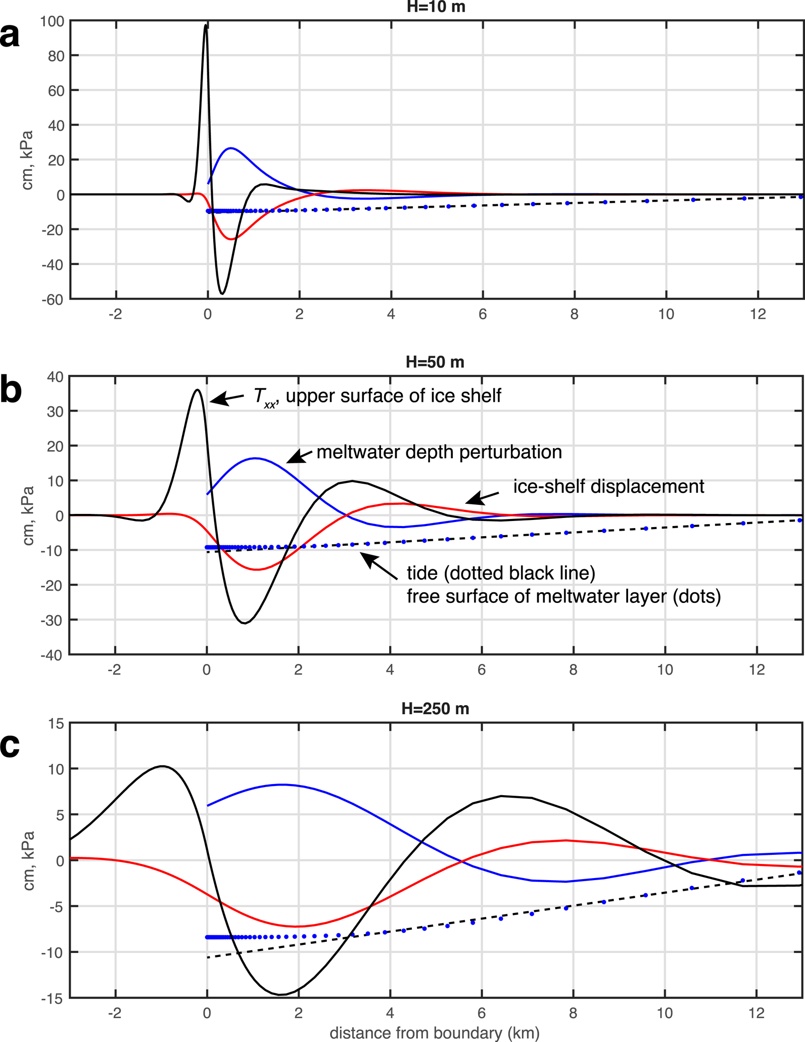
Fig. 10. Meltwater-layer depth perturbation (η, cm, blue line), ice-shelf deflexion due to purely elastic flexure (ζ, cm, red line), tide (T, cm, dashed black line), free-surface of meltwater layer (blue dots) and ice-shelf stress at the upper surface (T xx, kPa, black line) for three representative ice thicknesses (H = 10,50 and 250 m, panels (a–c), respectively). The time for which the solution is shown is π/4 units of phase after low tide (when the slope of T is maximum), and is chosen to show the depth of the meltwater-layer perturbation at its largest. Note the change in scale for each panel.
One of the key features of the elastic flexure of the ice shelf in response to the tidally forced meltwater fluctuations is the creation of flexure stresses which, as a result of the thin-plate approximation, are strongest, and of opposite sign, at the upper and lower ice-shelf surfaces (the upper and lower skin surface) and which vary linearly with vertical distance in the ice shelf. Figure 11 displays the maximum tensile stress attained at the upper surface of the ice shelf as a function of ice thickness (varying from 5 to 500 m) and for a variety of rheological treatments. The five rheological treatments are: (1–3) pure elastic, with E = 1,5,10 GPa, representing the range of natural ice, and (4–5) viscoelastic (following the method of MacAyeal and others, Reference MacAyeal, Sergienko and Banwell2015), with E = 5 GPa and ν = 1 × 10¹³ and 2.2 × 10¹⁴ corresponding to Maxwell times of about 30 min and 12.42 h (the M2 period), respectively.) The maximum tensile stress T xx achieved in the 1-D numerical model used to derive the results in Figure 10 increases with increasing Young's modulus (E) but decreases with H, as is displayed by the rightward decay of the curves in Figure 11. The flexural rigidity in the purely elastic treatment, D, is proportional to EH 3; so the decay with increasing ice thickness reflects the fact that the length scale over which non-zero bending moments are induced in the ice shelf by the shifting meltwater load is an increasing function of H. Only oneviscoelastic example is shown, and is produced for an unrealistically low ice viscosity (1013 Pa s) associated with an unrealistically short Maxwell time ν/E of approximately 30 min. For Maxwell times at or above the diurnal and semidiurnal tidal periods, the viscoelastic behavior is indistinguishable from the purely elastic behavior.

Fig. 11. Maximum tensile stress achieved at the time of greatest meltwater-layer depth as a function of ice thickness H and for various values of the Young's modulus E under the assumption of pure elastic rheology. Two viscoelastic solutions are also plotted. One with E = 5 GPa and a Maxwell time of 12.42 h (the periodicity of M2) plots exactly above the line for the purely elastic case with E = 5 GPa. The second with E = 5 GPa and assuming an ice viscosity of 1 × 10¹³ Pa s (an extremely low value, corresponding to a Maxwell time of 0.55 h) is located between the two elastic cases of E = 1,5 GPa. The maximum tensile stress is achieved at the surface of the ice shelf at the boundary of the meltwater regime near x = 0.
The magnitude of the maximum tensile flexure stress of the ice shelf may exceed what may be capable of producing fracture in the skin (upper surface) of the ice shelf (Banwell and others, Reference Banwell, MacAyeal and Sergienko2013). This is particularly significant given the fact that this tensile stress is cyclic and thus giving rise to the possibility of fatigue failure which occurs at stress levels that are reduced below the fracture criterion for time-independent stresses. Although the 1-D results shown in Figure 11 are idealized both in terms of geometry and tidal forcing (e.g. the meltwater-layer extends infinitely in the direction perpendicular to x, and the tidal-tilt magnitude dT/dx = 10−5 is at the high-end of what is feasible in natural settings), ice shelves with an effective elastic plate thickness of ~50 m or less will experience ~50 kPa tensile stresses (in their skin) repeatedly with each tidal cycle. This suggests that tidally induced flexure stresses due to movement of surface meltwater will have a bearing on the stability of thin ice shelves such as the McMIS (which ranges between 20 and 100 m in thickness, Rack and others, Reference Rack, Haas and Langhorne2013). Thick ice shelves, even ones with extensive surface meltwater systems, such as the Larsen B Ice Shelf prior to its 2002 collapse, will experience maximum tensile stresses on the order of 5–20 kPa, which are roughly 5–20% of the single-cycle fracture criterion of ~100 kPa. Cyclic stresses in the 10% range, after sufficient number of cycles, could be sufficient to fracture an ice shelf as is consistent with the basic principles of fatigue failure.
APPENDIX C. Estimation of tidal tilt on the McMurdo ice shelf
Over ice-shelf covered seas at locations distant from coasts and grounding lines, dry firn-covered ice shelves ride passively atop the ‘ocean-scale’ barotropic tidal waves that make up the semidiurnal, diurnal and long-period response of the global ocean to the astronomical tide potential (Platzman, Reference Platzman1978; Henderschott, Reference Henderschott1980). Counterintuitively, the great thickness of the ice shelf, sometimes far thicker than the ocean layer which is trapped below it, does little to influence the propagation of the ocean tide beyond determining the effective depth of the ocean (actual seabed depth minus ice-shelf draft) and providing a second rigid surface at which to generate friction (along with the sea bed). This characteristic results from the fact that long-period barotropic ocean tides propagate as shallow water waves (MacAyeal, Reference MacAyeal1984; Padman and others, Reference Padman, Erofeeva and Joughin2003b, Reference Padman, Siefgried and Fricker2018) for which vertical inertia of the ice and ocean beneath exerts a negligible influence on pressure (Pedlosky, Reference Pedlosky1987; Hutter and others, Reference Hutter, Wang and Chubarenko2014). For shallow water waves, only horizontal components of inertia are relevant, and horizontal motions of ice shelves driven by tide are easily disregarded when considering tidal wave propagation (Brunt and DR, Reference Brunt and MacAyeal2014).
Near coasts and grounding lines, however, the effect of the ocean-scale tide on vertical ice-shelf motion is complicated by at least four factors: (1) elastic rigidity of the ice shelf leading to flexural boundary layers within ~10 km of grounding lines (e.g. Vaughan, Reference Vaughan1995; Rosier and others, Reference Rosier2017), (2) decreasing water depth and increasing friction as the water column trapped between the sea bed and the ice-shelf narrows (Georgas, Reference Georgas2012; Rosier and others, Reference Rosier, Green, Scourse and Winkelmann2014), (3) the effects of nonlinear inertia terms that create asymmetry and generate harmonics (Aubrey and Speer, Reference Aubrey and Speer1985; King and others, Reference King2011), and (4) local resonance (Arbic and others, Reference Arbic, Karsten and Garrett2009). These effects generate perturbations from the large-scale character of the ocean-scale tidal wave propagation which are typically restricted to relatively small coastal regions. The rapidly increasing thickness of the ice upstream of a grounding line inhibits the rise and fall of the ice shelf near the grounding line, which leads to a kilometer-scale boundary layer along the grounding line where the ocean-scale tide is damped to zero by viscoelastic forces in the ice (e.g. Fricker and Padman, Reference Fricker and Padman2006; Walker and others, Reference Walker2013; Rosier and others, Reference Rosier2017).
Ice-shelf tilt is defined by $\nabla \zeta$ , where ζ is the perturbation of the neutral surface of the ice shelf (typically half way between the surface and bottom) about which elastic and viscoelastic deformation occurs, and where ∇ is the gradient with respect to horizontal coordinates. This tilt has a small component caused by the ocean-scale tidal wave in regions away from coasts and a large component caused by processes operating in grounding zones and where water-column thickness is restricted. Ocean-basin scale tilt is caused by two factors: (1) the variation of tidal phase in the direction of tidal-wave propagation and is typically parallel to the basin-scale trend of the ocean coastline (e.g. Platzman, Reference Platzman1978; Henderschott, Reference Henderschott1980), and (2) variation of tidal amplitude in a direction perpendicular to the coast caused by both coastal amplification due to shallowing and the effects of Earth's rotation (Pedlosky, Reference Pedlosky1987). The Kelvin wave (Platzman and others, Reference Platzman, Curtis, Hansen and Slater1981; Pedlosky, Reference Pedlosky1987) is a good idealized model of what the ocean tide looks like. These two variations are seen, for example, in the dominant semidiurnal M2 tide's amplitude and phase maps for the Southern Weddell Sea (Robertson and others, Reference Robertson, Padman and Egbert1985; Padman and others, Reference Padman, Fricker, Coleman, Howard and Erofeeva2003a, Reference Padman, Siefgried and Fricker2018; King and others, Reference King2011) and in the dominant diurnal K1 tide's amplitude and phase maps for the entire Southern Ocean (Platzman and others, Reference Platzman, Curtis, Hansen and Slater1981; Padman and others, Reference Padman, Siefgried and Fricker2018). The wavelength of the large-scale, ocean-scale tide is typically >6000 km; thus, for a tidal amplitude of 1 m, the maximum tilt in the direction of propagation is about 10−7, or about 1 cm in 100 km. Maximum tilt in the direction perpendicular to phase propagation is determined by the Rossby radius of deformation (Pedlosky, Reference Pedlosky1987), ${\sqrt {gh}}/{f}$
 , where g is the acceleration of gravity at the Earth's surface, h is mean water-column thickness (depth in open water) and f is the magnitude of the Coriolis parameter for the latitude in question, as well as by small-scale energy continuity considerations associated with varying h. For the Weddell Sea, the typical scale of tide variation perpendicular to the coastline is about 1 cm in 1–10 km (Robertson and others, Reference Robertson, Padman and Egbert1985; Padman and others, Reference Padman, Fricker, Coleman, Howard and Erofeeva2003a; Mueller and others, Reference Mueller2012; Zaron, Reference Zaron2018). This implies a tilt of about 10−5 to 10−6.
In the kilometer-scale boundary layer associated with grounding zones, ice-shelf tilt is on the order of 10's of cm per kilometer or 10−4 (e.g. Rosier and others, Reference Rosier2017). The grounding zone thus corresponds to a location where surface slopes can be as large as for ablation zones at the edges of the Greenland ice sheet. The tilt in the grounding zone is also the largest sea-surface tilt in the World Ocean, exceeding, for example the slope of dynamic topography, ~ 10−5, at the edges of the Gulf Stream off the Eastern coast of North America (Knudsen and others, Reference Knudsen, Bingham, Andersen and Rio2011; Rosier and others, Reference Rosier2017). While little has been done to observe tide asymmetry and harmonic excitation in ice-shelf-covered seas, observations of such phenomena elsewhere suggest that these effects could lead to centimeter-scale variation of ice-shelf surface elevation over kilometer-scale horizontal distances, thus also about ~ 10−5 (e.g. Aubrey and Speer, Reference Aubrey and Speer1985).
On discovering the diurnal variability in meltwater depth at Rift Tip Lake, the question we considered first was whether the cause could be the large-scale ocean tide in the Ross Sea, which is primarily diurnal (MacAyeal, Reference MacAyeal1984; Padman and others, Reference Padman, Fricker, Coleman, Howard and Erofeeva2003a, Reference Padman, Erofeeva and Joughin2003b). To investigate whether an ice-shelf surface tilt was associated with the tide propagating through McMurdo Sound, we examined GPS data we collected during the 2016/17 field season when the GPS array covered a larger area. GPS data collected in 2015/16 were from an array that was horizontally confined (within 1 km) and thus unable to allow a tilt signal to emerge from the GPS noise (of several centimeters). (We use the 2016/17 data because the location of GPS receivers in the second field season was more optimal for detecting tidal amplitude variation, and because the tidal propagation in McMurdo Sound is likely to not vary significantly from year to year.) Two GPS stations (labeled 1 and 2 in Fig. 2B, and identified as Ring GPS3 and Peanut GPS3 in Banwell and others, Reference Banwell, Willis, Macdonald, Goodsell and MacAyeal2019) are also located on the relict superimposed lake ice that now forms pedestals that rise above the ice-shelf surface due to differential ablation (Macdonald and others, Reference Macdonald2019), which is where we expect the GPS data to be least influenced by water movement during the early melt season (i.e. we expect these stations to reflect the tidal motion of the ice shelf without the influence of flexure in response to water loads). Description of the GPS measurements, data processing and uncertainty is provided in Banwell and others (Reference Banwell, Willis, Macdonald, Goodsell and MacAyeal2019).
Figure 12a shows the GPS height above geoid (mean value subtracted and smoothed with a 3-h running mean) and (bottom panel) the difference between GPS1 and GPS2 as a function of the height above geoid at GPS1. The result of fitting a line through the noisy GPS data in Figure 12b suggests that the tide amplitude differs by about 2 cm between Ring Lake (greater amplitude) and Peanut Lake (lesser amplitude). These two stations are about 3 km apart. This variation in tidal amplitude forms the basis for our use of 0.5 (≈2/3) cm per km as the tidal tilt in the vicinity of Rift Tip Lake for the exploratory numerical experiments conducted in this study.

Fig. 12. (a) Comparison of GPS-observed elevation over a 4-d period (13–17 January 2017) between Ring and Peanut lake GPSs (GPS 1 and 2 in Fig. 2b, also named Ring GPS3 and Peanut GPS3 in Fig. 1 of Banwell and others, Reference Banwell, Willis, Macdonald, Goodsell and MacAyeal2019). (b) Difference between GPS elevations at Ring and Peanut against tidal elevation at Ring over the 4-d period. Blue line indicates zero difference, red line indicates a least squares fit through all data points suggesting that the tidal amplitude is approximately 2 cm greater at Ring than at Peanut. The two GPS stations are 3.1 km apart. This forms an observational basis for our use of 0.5 (≈2/3) cm/km as the tidal tilt in the numerical experiments of this study.


 Open access