


1. INTRODUCTION
Mountain glaciers are the water towers of the world (Viviroli and others, Reference Viviroli, Dürr, Messerli, Meybeck and Weingartner2007). Although only covering ~3% of the earth's total glacierized land area (Meier, Reference Meier1984; Arendt and others, Reference Arendt, Echelmeyer, Harrison, Lingle and Valentine2002), small glaciers and ice caps (excluding the Antarctic and Greenland ice sheets) play an important role in assessing and predicting sea level change on decadal to centurial timescales (Oerlemans and Fortuin, Reference Oerlemans and Fortuin1992). Previous studies have indicated that these glaciers, whose shrinkage has tended to accelerate with the ongoing climate warming (Kaser, Reference Kaser1999; Arendt and others, Reference Arendt, Echelmeyer, Harrison, Lingle and Valentine2002; Paul and others, Reference Paul, Kääb, Maisch, Kellenberger and Haeberli2004; Meier and others, Reference Meier2007; Yao and others, Reference Yao2012), contributed ~20–60% to rising sea level in different periods (Meier, Reference Meier1984; Kaser and others, Reference Kaser, Cogley, Dyurgerov, Meier and Ohmura2006; Meier and others, Reference Meier2007; Gardner and others, Reference Gardner2013). Small glaciers have a shorter response time to climate change than the large ice sheets of Greenland and Antarctica, and their contribution may be even more if the climate continues to warm (Oerlemans and Fortuin, Reference Oerlemans and Fortuin1992). Variations in mountain glaciers are acknowledged to be among the best natural indicators of climate change. In contrast to variations in glacier length or area, variations in mass balance and equilibrium line attitude (ELA) are direct responses to glacier mass and climate change (Bolch and others, Reference Bolch2012).
Modeling is one of the major techniques for assessing glacier mass balance and ELA. The energy-balance and degree-day models are two widely applicable methods. Energy-balance models can describe the physical processes of a glacier surface in detail, but their parameters and input data are not readily available due to observational restrictions. On the contrary, degree-day models rely upon the relationship between snow or ice melt and positive temperatures (Hock, Reference Hock2003). On account of the wide availability and easy interpolation of air temperature data, the models are widely used in mass-balance estimation for a single glacier (Jóhannesson and others, Reference Jóhannesson, Sigurdsson, Laumann and Kennett1995; Braithwaite and Zhang, Reference Braithwaite and Zhang2000; Pellicciotti and others, Reference Pellicciotti2005; Azam and others, Reference Azam2014; Gao and others, Reference Gao2015; Liu and Liu, Reference Liu and Liu2016). At present, the distributed degree-day models are subjected to the considerable simplification that is necessary for operation at large scales (e.g., global or regional), and for estimation of the contribution of glaciers to sea level change (Raper and Braithwaite, Reference Raper and Braithwaite2006; Radić and Hock, Reference Radić and Hock2011; Marzeion and others, Reference Marzeion, Jarosch and Hofer2012; Giesen and Oerlemans, Reference Giesen and Oerlemans2013; Slangen and others, Reference Slangen2016). The simulated accuracy of degree-day models often outperforms energy-balance models on a catchment scale (Hock, Reference Hock2003).
The Beida River is located in an arid and semi-arid region in northwest China. In the catchment, glaciers are significant contributors to streamflow, serving as a frozen reservoir that supplements runoff during warm and dry periods. Approximately 15% of the runoff is from glaciers, and the rate will increase with the ongoing climate warming. The accelerated glacier retreat has significant implications for downstream oasis farming, regional water supplies and the sustainability of aquatic ecosystems (Shi and Zhang, Reference Shi and Zhang1995; Wang and others, Reference Wang, Li and Chen2001; Yang and others, Reference Yang, Ding and Shen2004; Liu and others, Reference Liu, Ding and Zhang2006). A study on glacier mass variation and its effect on surface runoff in Beida River catchment has important theoretical and practical significance. In the present study, using in-situ measured data from Qiyi Glacier and meteorological and run-off data from stations, we developed a distributed degree-day model at 1 d temporal resolution and 90 m spatial resolution. The aims of this study are to reconstruct the time series of mass balance and ELA in the Beida River catchment from 1957 to 2013, analyze the causes of glacier mass balance and ELA changes and discuss the essential relationships between glaciers, climate and runoff.
2. STUDY AREA, DATA AND METHOD
2.1. Selection of study area
The Beida River catchment (97°~99.5°E, 38°~40°N) is located in the upper reaches of the Heihe River (Fig. 1), which is the second biggest inland river in China. There are three tributaries in the catchment, from east to west, the Fengle River, Hongshui River and Tuolai River, with drainage areas of 565, 1578 and 6706 km2, respectively. Glacier meltwater has played a significant role in the development of downstream industry and agriculture. In the present study, we investigated a total of 631 glaciers, which had a total estimated area of 318.2 km2 and an average area of 0.5 km2. The glaciers are small in size; 87.6% of glaciers are <1 km2, and only two glaciers are >5 km2.

Fig. 1. Location of the Beida River catchment and observation in Qiyi Glacier.
Qiyi Glacier (39.5°N, 97.5°E) is located in the northwest of the Beida River catchment, and its meltwater flows into the Liuquangou River, which is a branch of the Tuolai River. This glacier has an interrupted observational time series spanning more than 20 years (1975–78, 1985–88 and 2000–13), and has good representation in the study area. Regional representation was based on the following criteria: (1) glacier is small in size, and the area is only 2.76 km2 (Pu and others, Reference Pu2005); (2) corresponding to 4003 m (minimum), 5531 m (maximum) and 4759 m (mean) of the glaciers elevation in the Beida River catchment, the elevation of Qiyi Glacier is from 4304 m in the terminus to 5159 m in the peak, and the average elevation is 4807 m; (3) corresponding to 25.7° of the average glaciers slope in the catchment, the average slope of Qiyi Glacier is 20°; (4) 32.3% of the glaciers in the catchment, which is the highest percentage, have the same aspect as the Qiyi Glacier (northwest); (5) according to the physical characteristics of glaciers, the Qiyi Glacier is classed as a sub-continental glacier, which is the same as most glaciers in the catchment.
2.2. Data
The datasets used in this study include: meteorological data, satellite data, field-based measurements from Qiyi Glacier and hydrological data.
2.2.1. Meteorological data
Five meteorological stations (Table 1, Fig. 1) around the catchment were selected, and meteorological data included the daily air temperature, precipitation, relative humidity, barometric pressure and sunshine duration. Among them, the data from a mountain meteorological station (Tuole) was used for driving the model and the rest were used for analyzing the response of glaciers to climate change. The datasets were derived from the China Meteorological Data Sharing Service System (http://data.cma.cn/).
Table 1. Meteorological and hydrological stations in this study

2.2.2. Satellite data
Considering the variations in glacier area from 1957 to 2013, glacier boundaries used in the model were distinguished into two periods: glacier boundaries between 1957 and 1985 were extracted from topographic maps of the 1970s; and glacier boundaries between 1986 and 2013 were taken from a satellite image from 2000. Fifteen topographic maps (1: 100 000) from the 1970s that were derived from aerial photographs taken by the Chinese Military Geodetic Service were selected. The satellite imagery was one Landsat TM image (P133 r33, 2000–5–20) that was taken in cloud-free conditions, with a spatial resolution of 30 m (http://www.usgs.gov/). The pretreatment of topographic maps included scanning, creating mosaics and Image registration; the Image registration and geocorrection of satellite imagery were accomplished in ArcGIS 9.3 software. Glacier boundaries were extracted by visual interpretation. A DEM of the catchment was derived from the Shuttle Radar Topography Mission, with a resolution of 90 m. The DEM was used to compute the following morpho-topographic variables of each glacier: average elevation, slope, aspect, latitude and longitude of the glacier centroid. All maps and images were projected into the Universal Transverse Mercator coordinate system referenced to the 1984 World Geodetic System.
2.2.3. Field-based measurements in Qiyi Glacier
The datasets included mass balance data, air temperature and precipitation data from different altitude intervals, and meteorological data from an automatic weather station (AWS). The mass balance measurement and calculation were using the same methods presented by Yao and others (Reference Yao2012). A monthly observation of mass balance was carried out from July 2011 to August 2013. Synchronously, air temperature and precipitation from different altitude intervals were measured by seven pairs of hygrothermographs and rain gauges (Fig. 1). The AWS was located at an altitude of 4763 m a.s.l.. Observed items of the AWS included wind speed and direction, air temperature, relative humidity, barometric pressure, snow depth and 4-component radiation (incoming and reflected shortwave radiation, incoming and outgoing longwave radiation). All of the above datasets were used for calibrating the parameters in the model, and mass balance and ELA data quoted from the papers published in the referred journals were used for validating the simulated results (Wang and others, Reference Wang, Xie and Wu1984, Reference Wang, Pu and Wang2011; Liu and others, Reference Liu, Xie and Yang1992; Pu and others, Reference Pu2005; Wang and others, Reference Wang, Pu and Wang2011; Yao and others, Reference Yao2012).
2.2.4. Hydrological data
The Binggou, Xindi and Fengle hydrological stations were respectively, located in the Tuolai River, Hongshui River and Fengle River catchments (Table 1, Fig. 1), which controlled the surface runoff of each river. Annual and monthly run-off data of the Binggou, Xindi and Fengle hydrological stations from 1957 to 2013 were selected to discuss the essential relationships between glaciers and runoff. The datasets were derived from the China Hydrological Almanac and Environmental and the Ecological Science Data Center in Western China (http://westdc.westgis.ac.cn/).
2.3. Method
2.3.1. Model description
The distributed degree-day mass-balance model in the Beida River catchment can be described over any period of time with the following formula (Oerlemans and Fortuin, Reference Oerlemans and Fortuin1992):
 $$B = \int _t \left[ {(1 - f)m + P_{\rm s}} \right]dt$$
where B (mm w.e.) is the glacier mass balance; f (f = 0.076) is the fraction of refreezing meltwater that is calculated by a multilevel snowmelt model (Yang and others, Reference Yang2013); m (mm w.e.) is the ablation water equivalent of ice and snow; P s (mm w.e.) is the accumulation which is equal to solid precipitation; and t is the selected period.
An improved degree-day model (Pellicciotti and others, Reference Pellicciotti2005) was used to simulate ice and snowmelt:
 $$m = \left\{ \,{\matrix{{ TF \cdot T + SRT \cdot (1 - \alpha ) \cdot S_{in}^i \; \; \; \; \; \; \; \; \; \; \; \; \; \; \; \; \; \; T \gt 0} \cr {\; \; \; \; \; \; \; \; \; \; \; \; \; \; \; \; \; \; \; 0\; \; \; \; \; \; \; \; \; \; \; \; \; \; \; \; \; \; \; \; \; \; \; \; \; \; \; \; \; \; \; \; \; \; \; \; \; \; T \le 0\;} \cr}} \right.$$
where TF (mm°C−1 d−1) and SRT (m2 mm W−1 d−1) are the degree-day factors. TF and SRT, which are obtained by using the multiple linear regression method, are different for different underlying surfaces (for ice, TF = 4.52, SRT = 0.0035; and for snow, TF = 1.64, SRT = 0.0075); T (°C) is the daily average air temperature 2 m above glacier surface; α is the albedo; and
 $S_{in}^i $
(W m−2) is the incoming shortwave radiation at a given grid cell (i) on the glacier surface.
$S_{in}^i $
(W m−2) is the incoming shortwave radiation at a given grid cell (i) on the glacier surface.
The incoming shortwave radiation
 $(S_{in}^i )$
is constituted by the direct radiation (I) and diffuse radiation (D). The partitioning between direct and diffuse radiation depends linearly on cloudiness, and the fraction of diffuse radiation (D
F) can be calculated (Oerlemans, Reference Oerlemans1992; Brock and Arnold, Reference Brock and Arnold2000; Sicart and others, Reference Sicart, Hock, Ribstein, Litt and Ramirez2011):
$(S_{in}^i )$
is constituted by the direct radiation (I) and diffuse radiation (D). The partitioning between direct and diffuse radiation depends linearly on cloudiness, and the fraction of diffuse radiation (D
F) can be calculated (Oerlemans, Reference Oerlemans1992; Brock and Arnold, Reference Brock and Arnold2000; Sicart and others, Reference Sicart, Hock, Ribstein, Litt and Ramirez2011):
 $$D_{\rm F} = 0.65n + 0.15$$
 $$\displaystyle{n = {{S_{in}^{Tuole}} \over K}}$$
where n is the cloudiness. For total cloud cover, 80% of the global radiation diffuses, whereas for clear-sky conditions it is only 15%.
 $S_{in}^{Tuole} $
is the incoming shortwave radiation at Tuole station, and these data are from the Institute of Tibetan Plateau Research, Chinese Academy of Sciences (ITPCAS) radiation forcing data (http://dam.itpcas.ac.cn/rs/?q=data). K is the potential direct solar radiation at the glacier surface without clouds, which is calculated as (Hock, Reference Hock1999):
$S_{in}^{Tuole} $
is the incoming shortwave radiation at Tuole station, and these data are from the Institute of Tibetan Plateau Research, Chinese Academy of Sciences (ITPCAS) radiation forcing data (http://dam.itpcas.ac.cn/rs/?q=data). K is the potential direct solar radiation at the glacier surface without clouds, which is calculated as (Hock, Reference Hock1999):
 $$K = I_0 \cdot \left( {\displaystyle{{R_{\rm m}} \over R}} \right)^2 \cdot {\rm \psi} _a^{\left( {\displaystyle{P \over {P_0 \cos Z}}} \right)} \cdot \cos {\rm \theta} $$
where I 0 (1362 W m−2) is the solar constant; (R m/R) is the correction factor of earth's orbit eccentricity; R is the instantaneous earth-sun distance; R m is the average earth-sun distance; ψa is the average atmospheric clear-sky transmissivity, with a value of 0.6 or 0.7 generally; P 0 (1013.25 hPa) is the standard atmospheric pressure; P (hPa) is the atmospheric pressure at different altitudes; Z is the local zenith angle; and θ is the angle of incidence between the normal to the grid slope and the solar beam.
The direct radiation (I) at a given point on a glacier surface without terrain shading could be calculated (Arnold and others, Reference Arnold, Willis, Sharp, Richards and Lawson1996):
 $$\eqalignno{I & = (1 - D_{\rm F} ) \cdot \vec S_{in} \cdot [\sin Z\cos \beta\cr &\quad + \cos Z\sin \beta \cos (\varphi_{sun} - \varphi _{aspect} )]}$$
where β is the slope angle, φ
sun
and φ
aspect
are the solar azimuth and the slope azimuth (aspect) angle, respectively.
 $\vec S_{in} $
is the normal incident direct solar radiation at the same point:
$\vec S_{in} $
is the normal incident direct solar radiation at the same point:
 $$\vec S_{in} = S_{in}^{Tuole} /\sin Z$$
The diffuse radiation (D) is constituted by the diffuse radiation in the sky and shortwave radiation reflected by the surrounding terrain:
 $$D = D_0 \cdot V_{sky} + \alpha _m \cdot \vec S_{in} \cdot (1 - V_{sky} )$$
where D 0 is the diffuse radiation in the sky without the terrain shading; α m (α m = 0.3) is the average albedo of the surrounding terrain; and V sky is the view factor of sky. If V sky = 1, the given grid cell was not shaded by the surrounding terrain; on the contrary, if V sky = 0, the grid cell was shaded. In this study, the terrain shading effect is determined by the ray tracing method (Arnold and others, Reference Arnold, Willis, Sharp, Richards and Lawson1996).
Albedo is among the key indicators of simulated accuracy. The albedo of the glacier surface is closely related to the number of days after snow. On one hand, the number of days after snow reflects the metamorphism of snow with time; on the other hand, it also reflects the accumulation effect of surface contamination over time. In this study, we used a parameterization scheme proposed by Oerlemans and Knap (Reference Oerlemans and Knap1998):
 $$\alpha ^{(i)} = \alpha _{snow}^{(i)} + (\alpha _{ice} - \alpha _{snow}^{(i)} )exp\left( {\displaystyle{{ - d} \over {d^{^\ast}}}} \right)$$
where α (i) is the albedo at a given grid cell (i) in glacier surface; d (cm) is the snow depth; d* (d* = 1.91 cm) is a characteristic scale for snow depth; and α ice is the albedo of ice, which is calculated by the following formula (Mölg and others, Reference Mölg, Cullen, Hardy, Kaser and Klok2008):
 $$\alpha _{ice} = aT_{\rm c} + b$$
where T c is the dew point temperature; a (a = 0.075) and b (b = 0.13) are constants; the albedo of snow surface α snow (i) is determined by the number of days after snow:
 $$\alpha _{snow}^{(i)} = \alpha _{\,firn} + (\alpha _{\,fresnow} - \alpha _{\,firn} )exp\left( {\displaystyle{{s - i} \over {t^{^\ast}}}} \right)$$
where α firn (α firn = 0.7) is the albedo for firn, α frsnow (α frsnow = 0.91) is the albedo for fresh snow; s is the number of the day on which the last snowfall occurred; and t* (t* = 1.73) is the timescale for snow metamorphism. All the parameters are determined by the least squares method.
The solid precipitation is calculated by the threshold temperature method (Kang and others, Reference Kang, Cheng, Lan and Jin1999):
 $$P_{\rm s} = \left\{ {\matrix{ {\; P_{total} \; \; \; \; \; \; \; \; \; \; \; \; \; \; \; T \lt T_{\rm s}} \cr {\; \displaystyle{{T_{\rm r} - T} \over {T_{\rm r} - T_{\rm s}}} \cdot P_{total} \; \; \; \; \; \; \; \; \; T_{\rm s} \le T \le T_{\rm r} \; \;} \cr {0\; \; \; \; \; \; \; \; \; \; \; \; \; \; \; \; \; \; \; \; \; \; \; T \gt T_{\rm r}} \cr}} \right.$$
 $$P_{\rm r} = P_{total} - P_{\rm s} \; \; \; {\rm \;} $$
where P s, P r and P total (mm) are snow, rain and total precipitation, respectively; T s and T r are the threshold temperatures for snow/rain transition, with the values of −1.05 and 0.64°C, respectively (using the Monte Carlo method, which runs modeling for a total of 1000 times to yield the minimum of RMSD between measured and modeled mass balance of Qiyi Glacier).
2.3.2. Parameters calibration
According to the in-situ measurements of air temperature and precipitation at different altitudes on Qiyi Glacier from 2011 to 2012, the lapse rate of air temperature was 0.70°C (100 m)−1. The observed site with maximum precipitation was located at 4670 m a.s.l., where the annual precipitation was 410.5 mm. The observations were similar to measured results (0.73°C 100 m−1 and 485 mm−1) by Wang and others. (Reference Wang2009) in 2007/08. To improve the simulated precision, we used different temperature and precipitation lapse rates in different months and altitude intervals, and considered the temperature difference between non-glacial and glacial regions when calculating the lapse rates. The details are shown in Tables 2–4.
Table 2. Temperature difference between non-glacial and glacial regions in different months of Qiyi Glacier (°C)

Table 3. Lapse rates of temperature in different months and altitude intervals (°C (100 m)−1)

Table 4. Precipitation gradients in different months and altitude intervals (mm (100 m)−1 d−1)

2.3.3. Results validation
Figure 2a shows the simulated and observed annual balance of Qiyi Glacier. Simulations of annual balance were in accord with observations (correlation coefficient, R = 0.91), especially after 2006/07 (R = 0.98). The simulated and observed average mass balances were, respectively, −264 and −250 mm w.e. a−1, with a relative error of 5.7%, and the relative error reduced to 0.7% after 2006/07. In the monthly mass-balance simulation (Fig. 2b), the correlation coefficient between the simulated and observed monthly balance was 0.92. Simulated results of the cold season (October–April) were consistent with observations, but some errors occurred in the warm season (May–September). Simulated and observed average monthly balances were, respectively, −69.5 and −71.5 mm w.e., with a relative error of 2.8%. Figure 2c illustrates the comparison between the simulated and observed annual ELAs of Qiyi Glacier. The modeled ELA was consistently higher than the observed ELA, with an average altitude difference of 117 m. Snowdrift from the accumulation area to the firn basin is suspected as the main reason. The snow shift was affected by the special terrain of Qiyi Glacier, so this process was not considered in the model. That is why the modeled mass balance is consistent with observations, but modeled ELA is higher. In general, the model performed moderately well.

Fig. 2. Observed and simulated annual balance (a), monthly balance (b) and annual ELAs (c) of Qiyi Glacier.
3. Results
3.1. Temporal variability of glacier mass balance and ELA
Mass balance and ELA are both direct and reliable indicators of glacier status. For all 631 investigated glaciers in the Beida River catchment, the average mass balance for the study period was −272 ± 67 mm w.e. a−1 (n = 56, P < 0.001, 95% confidence interval), with an ice loss of 3.99 Gt in the last 56 years. The minimum mass balance occurred in 2012/13 (−1043 ± 306 mm w.e.) and the maximum occurred in 1982/83 (197 ± 97 mm w.e.), with a span of 1240 mm w.e.. Correspondingly, the average ELA was 4916 ± 55 m a.s.l. a−1 (n = 56, P < 0.001, 95% confidence interval). The highest average ELA occurred in 2012/13 (5280 ± 162 m a.s.l.) and the lowest ELA occurred in 1982/83 (4292 ± 276 m a.s.l.), with a span of 988 m. In the Fengle River, Hongshui River and Tuolai River catchments, the average mass balances were, respectively, −450 ± 77, −260 ± 66 and −252 ± 66 mm w.e. a−1 (n = 56, P < 0.001, 95% confidence interval), which increased gradually from east to west. Correspondingly, the average ELA of these three catchments was 4894 ± 48, 4923 ± 57 and 4916 ± 55 m a.s.l. a−1 (n = 56, P < 0.001, 95% confidence interval), respectively.
Figure 3 illustrates the interannual variations in mass balance and ELA. Over the whole simulated period, the mass balance for the Beida River catchment decreased with a trend of −7.6 mm w.e. a−2. Accumulated anomalies of annual balance first showed a wavelike increasing trend then decreased sharply, and the maximum occurred in 1992/93. Annual balance varied tremendously before and after 1992/93, and the average mass balance reduced from −161 to −479 mm w.e. a−1. The interannual variations in mass balance for the Fengle River, Hongshui River and Tuolai River catchments were similar, with reduction rates of 9.5, 7.5 and 7.3 mm w.e. a−2, respectively. Correspondingly, ELA rose by 242 m in the last 56 years, at a rate of 4.3 m a−1. Additionally, similar change rates of ELA were found for the sub-catchments, which were 4.2, 4.6 and 4.2 m a−1 for the Fengle River, Hongshui River and Tuolai River catchments, respectively.

Fig. 3. Interannual variations (box figure) and accumulated anomalies (solid line) in glacier mass balance (a) and ELA (b) for the Beida River catchment. For each year, the horizontal red bar represents the annual average of the sample, Box-and-whisker plots indicate the 10th and 90th percentiles (whisker caps), 25th and 75th percentiles (gray box ends), and median (solid middle bar).
Under the dominance of the Indian monsoons and westerlies, the seasonal variation in mass balance for glaciers in western China is distinctive (Yao and others, Reference Yao2012; Mölg and others, Reference Mölg, Maussion and Scherer2014). The warm season (May–September) dominates both ablation and accumulation for glaciers in the Beida River catchment (Fig. 4). Mass balance was slightly positive in the cold season (October–April), with an average of 7.1 mm w.e.. Ablation and accumulation over this period were both weak. The average monthly ablation was 2.4 mm w.e., while the monthly accumulation was 9.4 mm w.e.. Precipitation in the warm season (May–September) accounted for 80% of the annual total. However, the maximum accumulation occurred in June, rather than July or August. Snowfall during the summer could, with warming, fall as rain and the decrease in fresh snow would then reduce the glacier surface albedo, leading to greater ablation (Fujita and Ageta, Reference Fujita and Ageta2000; Fujita, Reference Fujita2008). Controlled by high temperature, ablation is most intense in July and August, with an average monthly ablation of 226.4 mm w.e.. The mass balance in May is the most positive because of the reduced ablation and moderate accumulation. Seasonal changes of mass balance in the three sub-catchments were similar to those of the Beida River catchment. Seasonal changes of mass balance were controlled by summer (June, July and August) temperature and the warm season (May–September) precipitation.

Fig. 4. Seasonal changes of ablation, accumulation and mass balance for glaciers in Beida River catchment.
3.2. Spatial variability of the mass balance and ELA
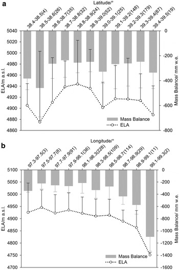
To investigate the spatial variability of mass balance and ELA for glaciers in the Beida River catchment, glacier distribution was classified into 11 latitude intervals (0.1°) and 10 longitude intervals (0.2°; Fig. 5). There is no clear trend with latitude (Fig. 5a). On the other hand, both mass balance and ELA decreased gradually with longitude from west to east. Mass balance changed 312 mm w.e. per degree of longitude, and the equivalent variation of ELA was 73 m.

Fig. 5. Spatial variability of glacier mass balance and ELA (the number in brackets is the number of glaciers in each interval, similarly hereinafter).
4. DISCUSSION
4.1. Reasons for variations of mass balance and ELA
4.1.1. The role of climate control
To explore the effect of climate control on glaciers around the study area, the annual air temperature and precipitation from meteorological stations were selected to analyze abrupt change, trend and persistence (Table 5, Fig. 6). Then, mass-balance sensitivities to climatic control were assessed.

Fig. 6. Average annual air temperature (a) and precipitation (b) in mountain and plain meteorological stations.
Table 5. Analysis of abrupt change, trend and persistence analysis for average annual air temperature and precipitation in five meteorological stations

* Unit of trend is mm a−1, and the number in bracket was the coefficient of determination (R 2).
Abrupt changes in the time series were analyzed by using the Mann–Kendall method (Hirsch and Slack, Reference Hirsch and Slack1984; Wei, Reference Wei2008), which is a non-parametric statistical test method. The results show an abrupt change of annual air temperature happened in the middle of the 1990s, and temperature continued to rise thereafter. Especially after 2000, the significance level of the warming trend vastly exceeded the 0.05 threshold value (α 0.05 = ± 1.96); thus, the warming trend was quite significant. Climate change was different between mountains and plains. The temperature difference in the mountain stations before and after the abrupt change year was 1.09°C, and 0.93°C in the plains stations. Assuming a continuous linear trend, the average annual air temperature rose by 0.295°C (10 a)−1 in the mountains, compared with 0.237°C (10 a)−1 in the plains. An abrupt change of annual precipitation happened in the early 1980s in the mountains, but in the middle of the 1980s in the plains (1970 at Gaotai station). Whether in the mountains or in the plains, the series had a non-significant increasing trend, with the growth rates of 15 mm (10 a)−1 in the mountains and 3.6 mm (10 a)−1 in the plains.
Long-range dependence generally existed in the climatic time series. The Hurst coefficient (H, 0 < H < 1) was used for quantitatively describing this long-range dependence, namely, persistence. The R/S method is one of the most common methods to estimate the Hurst coefficient (Rao and Bhattacharya, Reference Rao and Bhattacharya1999). The results showed all Hurst coefficients exceeded 0.5 (Table 5), which indicated the trend of the climatic time series had a strong persistence. The Hurst coefficients for annual temperature all exceeded 0.75, while they were only 0.5–0.7 for precipitation. Thus, warming and wetting would continue in the future. Compared with precipitation, the persistence of air temperature was stronger.
Mass-balance sensitivities refer to variations in mass balance caused by instantaneous changes in temperature and precipitation. Combined with the data on anomalies of temperature (ΔT) and precipitation (ΔP) in mountain meteorological stations, glacier mass change (ΔB) in the Beida River catchment over any given period can be computed by:
 $$\Delta B = \displaystyle{{\partial B} \over {\partial T}}\Delta T + \displaystyle{{\partial B} \over {\partial P}}\Delta P$$
where ∂B/∂T and ∂B/∂P are mass-balance sensitivities to temperature and precipitation change, respectively.
In the study area, the mass-balance sensitivities to temperature and precipitation change were, respectively, −239 mm w.e.°C−1 a−1 and +1.1 mm w.e. mm−1 a−1. That is, a 210 mm increase in precipitation was needed to compensate for the net mass loss induced by an air temperature increase of 1°C. According to the recent rates of increase of temperature (0.295°C 10 a−1) and precipitation (15 mm 10 a−1), the glacier mass balance in the Beida River catchment will reach −463 mm w.e. in the 2020s, and −627 mm w.e. in the 2050s.
4.1.2. The role of glacial morphological variables
With the warming and wetting in the Beida River catchment, glacier areas have varied considerably. The total area of the 631 investigated glaciers decreased from 318.2 to 275.3 km2, with a loss of 13.5% during 1970–2000. Thirteen glaciers, with a total area of 1.02 km2, had disappeared completely by 2000. Three new glaciers appeared by fragmentation of older ones. Glacial morphological variables played an important role in the variations of glacier mass balance and ELA. Mountain regions dominated by small glaciers are generally more sensitive to change (Bahr and others, Reference Bahr, Pfeffer, Sassolas and Meier1998). Figure 7 presents the relationship between mass balance (ELA) and initial glacier size (1970s) for 631 glaciers in the Beida River catchment. All 631 glaciers were classified into six size classes (<0.1, 0.1–0.5, 0.5–1, 1–2, 2–5 and >5 km2). The mass balance was more negative for small glaciers (<2 km2), and the mean was −254 ± 221, −279 ± 183, −286 ± 153 and −260 ± 147 mm w.e. in the <0.1, 0.1–0.5, 0.5–1and 1–2 km2 intervals, respectively. Mass balance increased when area exceeded 2 km2, and the average mass balance was −192 ± 74 and −165 ± 142 mm w.e. in the 2–5 and >5 km2 intervals, respectively. The ELA increased linearly with glacier area, at a rate of 9.2 m km−2.

Fig. 7. Relationships between initial glacier size (1970s) and mass balance (a) and ELA (b). Average values of glacier mass balance or ELA (red point) together with uncertainty ranges (whisker caps) are shown for six area classes (<0.1, 0.1–0.5, 0.5–1, 1–2, 2–5 and >5 km2).
4.1.3. The role of topographic variables
Mass balance increased linearly with altitude, at a rate of 128.7 mm w.e. (100 m)−1. Correspondingly, the trend of ELA with altitude presented first a rise then a drop instead of a monotonicity, and the highest average ELA was 4937 m a.s.l. in the 4700–4800 m interval (Fig. 8a). 90.6% of the glaciers had an average slope between 20° and 35°. Mass balance and ELA were similar in all six intervals except the 10°–15° interval. The difference between maximum and minimum of mass balance was 64 mm w.e., and 55 m of ELA (Fig. 8b). Among the eight aspects of glaciers (Fig. 8c), 501 glaciers faced north (north, northeast and northwest), accounting for 79.4% of the total number. The most negative mass balances, appearing in glaciers of these three aspects, were −412, −315 and −277 mm w.e., respectively. On the contrary, only 9% of the glaciers faced south, with an average mass balance of −28 mm w.e.. Average ELAs in all aspects were between 4860 and 4940 m a.s.l., and glaciers facing south and west had lower ELAs than glaciers facing north and east.

Fig. 8. Relationships between mass balance and ELA and average altitude (a), slope (b) or aspects (c) of glaciers in the Beida River catchment.
4.2. The relationship between mass balance and ELA
An excellent linear relationship (Fig. 9) existed between annual mass balance (B) and ELA (ELA t for the same year (t), Braithwaite (1984) described this relationship as:
 $$B_{\rm t} = {\rm \alpha} (ELA_0 - ELA_{\rm t} )$$
where ELA 0 is the balanced-budget ELA, i.e., when B t = 0, ELA t = ELA 0; and α is termed the effective balance gradient, as it represents a type of time- and space-average of the balance gradient. Regarding all 631 investigated glaciers in the Beida River catchment as a whole, the balanced-budget ELA (ELA 0) was 4687 m a.s.l., and the effective balance gradient (α) was 113.5 mm w.e. (100 m)−1. The effective balance gradient obviously changed in 2005/06, 2009/10 and 2012/13 (Fig. 9) when the mass balances (−745, −860 and −1043 mm w.e.) were the most negative. The reason was that the annual ELAs (5279, 5260 and 5280 m a.s.l.) in these 3 years had exceeded the top of 96.8% of the investigated glaciers.

Fig. 9. Relationship between annual mass balance and ELA.
4.3. Glacier meltwater runoff and potential effect on surface runoff
The average annual river runoff in the Beida River catchment was 9.74 × 10⁸ m3, and glacier meltwater runoff was 1.51 × 10⁸ m3, accounting for 15.2% of surface runoff (Table 6). Only the contribution in the Fengle River catchment was similar to that of the Beida River catchment. In the other two sub-catchments, the average annual glacier meltwater runoff was almost the same, but there was a difference in the roles of glaciers in supplying rivers. In the Hongshui River catchment, more than 1/4 of the surface runoff was derived from meltwater, while the proportion was only ~1/10 in the Tuolai River catchment.
Table 6. Average annual river runoff, glacier meltwater runoff and contribution during 1957–2013

As to the seasonal distribution (Fig. 10), meltwater runoff and surface runoff in the Beida River catchment were both concentrated in summer, especially in July and August. Seasonal variation presented a unimodal distribution, because high temperatures in summer dominated glacier ablation, and precipitation in summer accounted for 2/3 of annual precipitation. In wintertime (from October to March of the following year), meltwater was limited and surface runoff was homogeneous, with an average of 0.378 × 10⁸ m3. 92.3% of runoff during wintertime was derived from the Tuolai River, which was mainly supplied by base flow, such as spring water (Zhao and others, Reference Zhao2011). In the other two sub-catchments, although limited, the main water supply of runoff during wintertime was still glacier meltwater, and the contribution even exceeded 80% in some months. Consequently, groundwater was also an important component of the water supply in addition to glaciers and precipitation in Tuolai River catchment.

Fig. 10. Average monthly river runoff, glacier meltwater runoff and contribution in the Beida River catchment during 1957–2013.
Figure 11 illustrates the annual river runoff, glacier meltwater runoff and its contribution to the Beida River catchment during 1957–2013. Abrupt change and trend analysis were carried out by using the Mann–Kendall method. The results showed that annual runoff decreased insignificantly, at a rate of 0.011 × 10⁸ m3 a−1. The time series of glacier meltwater runoff changed abruptly in 2000, and the trend had a transition from a slow decrease to a rapid increase before and after 2000. Average annual meltwater runoff increased from 1.35 × 10 to 1.97 × 10⁸ m3, and the contribution to surface runoff increased from 13.9 to 20.4%. Therefore, the role of glacier meltwater supplying surface runoff was significantly strengthened with climate warming. Although average annual runoff declined slightly by 0.03 × 10⁸ m3 before and after 2000, the composition of runoff in different seasons changed considerably (Fig. 12). Surface runoff was mostly supplied by base flow (spring water) from November to May of the following year (Zhao and others, Reference Zhao2011), but monthly supply decreased by 0.056 × 10⁸ m3 (14.7%). Thus the role of groundwater supply was gradually weakened. Surface runoff increased by a total of 0.36 × 10⁸ m3 from June to October, which was principally caused by the increase of meltwater runoff in summer, with an increment of 0.59 × 10⁸ m3.
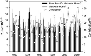
Fig. 11. Annual river runoff, glacier meltwater runoff and its contribution in Beida River catchment during 1957–2013.

Fig. 12. Average monthly river runoff, glacier meltwater runoff and contribution before and after 2000 in Beida River catchment.
5. CONCLUSIONS
Based on in-situ measurements on Qiyi Glacier, in combination with meteorological, hydrological and remote-sensing data, a distributed degree-day model at 1 d temporal resolution and 90 m spatial resolution was developed for the 631 investigated glaciers in the Beida River catchment. Utilizing this model, we reconstructed the time series of mass balance and ELA from 1957 to 2013. In parallel, we analyzed the factors that affected glacier mass balance and ELA, and discussed the essential relationships between glaciers and runoff. According to the above study, several facts were worth highlighting:
-
• The average mass balance was −272 ± 67 mm w.e. a−1, with an ice loss of 3.99 Gt during 1957–2013. Correspondingly, the average ELA was 4916 ± 55 m a.s.l. a−1; assuming a continuous linear trend, ELA rose by 242 m.
-
• Compared with morpho-topographic variables, climatic control is a more important factor affecting glaciers. A 210 mm increase in precipitation would be needed to compensate for the net mass loss induced by an air temperature increase of 1°C. Mass balance sensitivity to air temperature change was −239 mm w.e. °C−1 a−1, while sensitivity to precipitation change was +1.1 mm w.e. mm−1 a−1.
-
• The average annual runoff was 9.74 × 10⁸ m3 in the Beida River catchment during 1957–2013, and glacier meltwater runoff was 1.51 × 10⁸ m3, accounting for 15.2% of runoff. Series of annual meltwater runoff changed abruptly in 2000, and the contribution to runoff increased from 13.9 to 20.4% before and after 2000.
-
• Glacier meltwater and runoff were both concentrated in summer. Seasonal variation presented a unimodal distribution. With climate warming, the supply of meltwater was significantly increased in summer, with an increase of 0.59 × 10⁸ m3. The base flow, a dominating water supply in wintertime, had a gradually weakened role in supplying runoff.
ACKNOWLEDGEMENTS
This research was funded by the National Natural Science Foundation of China (No. 41190081; No. 41171056) and the Strategic Priority Research Program (B) of CAS (grant XDB03030208). We thank Zhang Huawei for providing topographical maps of the Beida River catchment, and all members of expedition in Qiyi Glacier from 2010 to 2012.


 Open access