


1. Introduction
The redistribution of snow by wind can play an important role in providing additional mass to the surface of ice masses. The effects of such snowdrift have been shown to be crucial in the distribution of snow on ice caps and ice sheets, where it can increase the heterogeneity of snow accumulation (Zwinger and others, Reference Zwinger, Malm, Schäfer, Stenberg and Moore2015) and can have a significant impact on glacier mass balance (Sauter and others, Reference Sauter2013). This variation in snow accumulation as a function of snowdrift could potentially help in interpreting buckled radio-echo sounding layers in Antarctica (as described by Siegert and others, Reference Siegert, Pokar, Dowdeswell and Benham2005), especially around the mountainous margins of the continent, as these are a function of accumulation rate, as well as ice flow and basal melting conditions. In areas of marginal (or niche) glaciation, local topoclimatic effects such as topographic shading or enhanced accumulation through avalanching and snowdrift may be crucial for the initiation and survival of glaciers. Reconstructions of former glacier limits have often been used to infer past climatic conditions (e.g. palaeotemperature or palaeoprecipitation) at the equilibrium line altitude (ELA) (e.g. Hughes, Reference Hughes2002; Carr and Coleman, Reference Carr and Coleman2007; Carr and others, Reference Carr, Lukas and Mills2010; Mills and others, Reference Mills, Grab, Rea, Carr and Farrow2012). However, the role of topoclimatic effects on the occurrence of small glaciers means that these glaciers could primarily reflect local climatic conditions rather than past regional climatic conditions. It is therefore important to understand the role of these local effects, to adequately assess whether palaeoclimatic reconstructions from former glaciers are an accurate representation of past regional climatic conditions, or whether reconstructed ELAs are substantially altered due to local factors such as snowdrift, which would then need to be accounted for in palaeoclimatic interpretations.
For example, much of the work undertaken in the British Isles regarding the reconstruction of former glaciers does not consider the implications of the role of snowdrift on the derived palaeoclimatic conditions (e.g. Lukas and Bradwell, Reference Lukas and Bradwell2010; Boston and others, Reference Boston, Lukas and Carr2015). When snowdrift has been considered, the studies have broadly followed the approach of Sissons and Sutherland (Reference Sissons and Sutherland1976) which considers that all ground lying above the ELA and sloping towards the glacier surface has the potential to contribute snow to the glacier surface. This method gives a good indication of the potential wind directions most likely to contribute snow to the former glacier surface. Mitchell (Reference Mitchell1996) and later Coleman and others (Reference Coleman, Carr and Parker2009), refined this method to take into account the uphill movement of wind-blown snow. But, this is still not a complete picture of snow redistribution.
Following Bell and Quine (Reference Bell and Quine1996), Purves and others (Reference Purves, Mackaness and Sugden1999) developed a snowdrift model in a GIS using a shelter index based on a digital elevation model (DEM), to demarcate areas of snow ablation and accumulation due to snowdrift processes. Purves and others (Reference Purves, Mackaness and Sugden1999) used the model to assess the potential contribution of wind-blown snow to formerly glaciated corries in the Cairngorms. However, this model has not been used subsequently. Despite the potential applicability of the Purves and others (Reference Purves, Mackaness and Sugden1999) model to any region and the recent advances in GIS and improved DEM accessibility, the Sissons and Sutherland (Reference Sissons and Sutherland1976) approach has remained the preferred method for reconstructing snow distribution in palaeoenvironments (e.g. Lewis and Illgner, Reference Lewis and Illgner2001; Coleman and others, Reference Coleman, Carr and Parker2009; Mills and others, Reference Mills, Grab, Rea, Carr and Farrow2012; Chandler and Lukas, Reference Chandler and Lukas2017).
Several other snowdrift models exist. These range from simple models, such as the drift routine in SNOWPACK (Lehning and others, Reference Lehning, Doorschot and Bartelt2000) to more sophisticated models such as SnowTran-3D (Liston and Sturm, Reference Liston and Sturm1998), PIEKTUK-D (Déry and Yau, Reference Déry and Yau2001), ALPINE3D (Lehning and others, Reference Lehning2006) and snow2blow (Sauter and others, Reference Sauter2013). SNOWPACK is a 1-D momentum, mass- and energy-balance model, while the more sophisticated models (SnowTran-3D, PIEKTUK-D, ALPINE3D and snow2blow), account for spatial and temporal snowdrift variations, incorporating saltation, turbulent-suspended transport and sublimation. These models provide snow depth measurements (w.e.), which can be converted to winter solid precipitation (Liston and Sturm, Reference Liston and Sturm2002). One of the main problems in the application of these models to palaeoenvironments is their requirement for meteorological inputs, including air temperature, precipitation and relative humidity. These are often unavailable for palaeoenvironments.
Snow transport due to gravitational processes, such as avalanching are particularly important in areas with steep inclines and can be responsible for substantial accumulation of snow at the base of steep slopes (Gruber, Reference Gruber2007; Bernhardt and Schulz, Reference Bernhardt and Schulz2010). Models that exist to replicate these processes include an algorithm which parameterises mass transport and deposition, to simulate avalanching in mountain environments (Gruber, Reference Gruber2007) and SnowSlide, which introduces lateral snow transport into an existing snowdrift model (Bernhardt and Schulz, Reference Bernhardt and Schulz2010).
The Purves and others (Reference Purves, Mackaness and Sugden1999) model differs from these approaches outlined above; it uses a series of rules to describe relative snow accumulation over complex terrain, rather than absolute snow accumulation depths, and so only basic meteorological inputs are needed. This relative snow accumulation field can then be used to create a ‘snowdrift index’ for any particular glacier system, ranking each system with respect to its neighbours to aid regional interpretation. The aim of the model is to determine the locations most likely to have had the greatest addition of mass through snowdrift rather that the quantitative estimates of the contribution of snow to former glacier surfaces. The advantage of this simpler approach by Purves and others (Reference Purves, Mackaness and Sugden1999) is that it requires fewer meteorological inputs. It is important, however, to be aware of its limitations, particularly relating to processes which are parameterised or omitted, such as sublimation and avalanching.
In this paper, we present a new and improved version of the Purves and others (Reference Purves, Mackaness and Sugden1999) snowdrift model, that we call Snow_Blow. We apply Snow_Blow to a contemporary glacial environment to assess the validity of its outputs and to increase confidence in its use in palaeoenvironmental settings. The model is written in the Python scripting environment in ESRI ArcGIS, which makes the model accessible to palaeoenvironmental researchers. The code is freely available online at GitHub and at https://doi.org/10.5281/zenodo.3336070.
To investigate the impact of snowdrift upon glaciers in future palaeoenvironmental settings, we first test Snow_Blow in a contemporary setting in Antarctica. We focus on four specific aspects: (1) testing the sensitivity of the results for a range of parameters, to determine how these impact model outputs for snow deposition (Section 5.1.1). (2) Assess snow erosion in comparison with the distribution of Blue Ice Areas (BIAs) (Section 5.1.2). This allows us to determine the likely number of iterations required to generate snow erosion that is comparable with BIAs, which allows for comparisons with other studies. (3) Undertake a quantitative assessment of parameter sensitivity to determine a most likely set for future model runs (Section 5.2). (4) Create a snowdrift index that takes into account catchment size on the importance of snowdrift, and thus identifies which localities are more susceptible to alteration by snowdrift depending on a particular wind direction (Section 5.3).
2. Snowdrift
Snow transport by wind, or snowdrift, can lead to a significant redistribution of the existing snow cover (Pomeroy and others, Reference Pomeroy1998; Balk and Elder, Reference Balk and Elder2000; Bowling and others, Reference Bowling, Pomeroy and Lettenmaier2004; Bernhardt and others, Reference Bernhardt, Zängl, Liston, Strasser and Mauser2009). Studies show that the major transport modes of snow are saltation and suspension (Budd and others, Reference Budd, Dingle, Radok and Rubin1966; Pomeroy and Gray, Reference Pomeroy and Gray1990), where wind must reach a certain threshold speed before snow particles are picked up and transported. This threshold speed is a function of the snow properties, and a range of estimates are recorded across the literature (e.g. Li and Pomeroy, Reference Li and Pomeroy1997, Liston and others, Reference Liston2000, Liston and others, Reference Liston2007, He and Ohara, Reference He and Ohara2017). Li and Pomeroy (Reference Li and Pomeroy1997) state that for dry snow, the range is on the order of 4–11 m s−1 ambient wind speed, with an average of ~7 m s−1, whereas Liston and others (Reference Liston2000) give a narrower range of 4–6 m s−1. Liston and others (Reference Liston2007) suggest that 4–5 m s−1 is a commonly used threshold velocity for dry snow. Transport by suspension can also lead to a loss of snow mass to the atmosphere, of the order of 15–25%, which is largely accounted for through sublimation (Pomeroy and others, Reference Pomeroy, Marsh and Gray1997; Bintanja, Reference Bintanja1998).
A generalised pattern of snow erosion on exposed sites such as ridge tops (where wind speeds are high), and snow deposition in sheltered sites such as the lee of ridges, and in topographic depressions (where wind speeds are reduced) can be observed in mountain environments (Benson and Sturm, Reference Benson and Sturm1993; Pomeroy and others, Reference Pomeroy, Gray and Landine1993; Liston and Sturm, Reference Liston and Sturm1998, Reference Liston and Sturm2002; Sturm and others, Reference Sturm, Liston, Benson and Holmgren2001; Mott and others, Reference Mott2008). Snow_Blow aims to reproduce these patterns of snowdrift by parameterising the above snowdrift processes, using a simple topographic-based shelter-index approach.
3. Study area
3.1. Ellsworth Mountains, Antarctica
We assess the validity of Snow_Blow in Horseshoe Valley, in the Heritage Range of the Ellsworth Mountains, Antarctica (Fig. 1). The mountains that define Horseshoe Valley in West Antarctica protrude 150–300 m above the present ice-sheet surface, reaching elevations of 1200–1600 m a.s.l. (Winter and others, Reference Winter2015). These mountains break an undisturbed wind fetch of several hundred kilometres, where katabatic winds, that evolve high on the Antarctic plateau (where net long-wave radiation losses cool the near-surface air (Nylen and others, Reference Nylen, Fountain and Doran2004)) replace the less dense air in Horseshoe Valley (Hoinkes, Reference Hoinkes1960; Ishikawa and others, Reference Ishikawa, Kobayashi, Ohtake and Kawaguchi1982). This phenomenon initiates and maintains BIAs in the lee of the Heritage Range, particularly along the leeward slopes of the Patriot and Independence Hills (Fig. 1). Landsat imagery reveals wind drift tails behind exposed rock (Fig. 1b), BIAs on the leeward slopes of the mountains, and snow accumulation in the lee of the mountains. These features highlight areas of net snow gain (drift tails and leeward areas) and net snow loss (BIAs), making this region ideal for validating the Snow_Blow model. This observed snow extent (Fig. 1d, inset) is delineated using a threshold reflectance value of 120 (8-bit image) in the blue band of the January 2009 Landsat image (see Burton-Johnson and others (Reference Burton-Johnson, Black, Fretwell and Kaluza-Gilbert2016) and Supplementary Section 5 for further information).
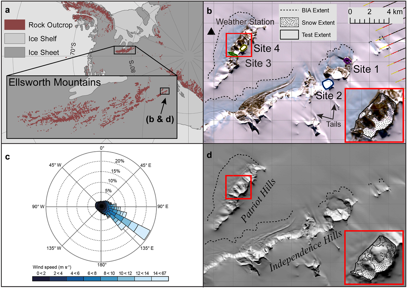
Fig. 1. Location map for the study site in the southern Heritage Range, West Antarctica. (a) Horseshoe Valley is situated at the southern extreme of the Ellsworth Mountains. Background imagery is from v5 of the Antarctic Digital Database (ADD). (b) Landsat 7 true colour composite of the Horseshoe Valley field site, from 21 September 2009. Lines in the imagery are the result of scan line issues with Landsat 7. The inset figure shows areas of mapped snow at sites 3 and 4. (c) Wind Rose showing wind direction data and wind speed from the privately operated Patriot Hills weather station, 2008–2009 (marked in panel 1b). (d) REMA (Howat and others, Reference Howat, Morin, Porter and Noh2018) for the study region, with annotation and inset as in (b). Wind drift tails and blue ice moraines are clearly visible. The dashed lines demarcate BIAs.
At this stage, we highlight the distinction between snow and ice ablation in BIAs. Once the snow is removed from the ice surface, ice ablation occurs through sublimation, which effectively draws older ice to the surface. In this paper, we focus on the surface snow processes, rather than ice ablation.
The advantages of using the Ellsworth Mountains for validation are threefold. (1) The katabatic winds blow from a consistent direction (Fig. 1c). (2) There is a clear demarcation of areas of high snow erosion (i.e. the BIAs and snow-free rock surfaces, Fig. 1b, inset) and low snow erosion/deposition in the lee of the mountains (Fig. 1). (3) We assume the snow ablation is solely due to wind-related processes, which eliminates the need to include sublimation processes that exist over coastal areas and BIAs in Antarctica. This eliminates the need to include enhanced melting variables that exist in alpine environments, which result from positive air temperatures and solar radiation. We appreciate that this region represents an extreme end-member environment with high wind speeds, and cold, dry conditions. The other potential disadvantage of validation in this area is that snow depth measurements have not been collected. However, the aim of this paper is to produce patterns of snowdrift and relative depths, so the pattern of blue ice (i.e. snow-free areas) in Horseshoe Valley in the southern Heritage Range forms an appropriate test for the Snow_Blow model.
To assess the assumption in point (3) we have compared the extent of BIAs downwind of the Patriot and Independence Hills, as well as the coverage of snow in the lee of the mountains, in temporally classified Landsat 7 and Landsat 8 imagery. These areas do not change much over time (Supplementary Fig. 1); specifically the 2008–2009 season, which coincides with meteorological data presented in this paper, is similar to the 2016–2017 and 2017–2018 austral summer seasons. Furthermore, there is no clear pattern of increased snow-free area towards the end of each summer season so the variation in extent of BIA over time is more likely to be a function of the time since the last snowfall event, rather than the time of year. These observations confirm that the assumption in point (3) above is an acceptable approximation because BIAs appear to be largely wind-driven features which show stability in extent over decadal time periods.
3.2. Input data
This study uses the REMA (Reference Elevation Model of Antarctica) Release 1 DEM (Fig. 1d), which is created from stereophotogrammetry, derived from DigitalGlobe satellite imagery (Howat and others, Reference Howat, Morin, Porter and Noh2018). Although the original DEM is supplied at an 8 m resolution, it is resampled in this study to a 30 m resolution to match the available Landsat imagery; this has the added advantage of decreasing the computational expense of the model. The other essential input to Snow_Blow is a dominant wind direction. Average hourly weather station data were recorded at the Patriot Hills blue-ice aircraft runway during 2008–2009 (data available at: https://geographic.org/global_weather/antarctica/patriot_hills_aws_890810_99999.html). These data show a modal wind direction of 122.5° when converted to polar stereographic grid angles. Mean wind speed is 8.1 m s−1, with a maximum value of 31.2 m s−1, and a std dev. of 5.0 m s−1 (Fig. 1c, Supplementary Fig. 2). As wind speeds higher than the mean can impact the pattern of snowdrift, a wind speed of 15 m s−1 was selected to represent these wind speeds in the period prior to the acquisition of the 2008–2009 Landsat imagery. This is an arbitrary choice and, as demonstrated later, different values can be tested as part of any application of the model.
4. Methodology
The Snow_Blow model presented here builds on the model developed by Purves and others (Reference Purves, Barton, Mackaness and Sugden1998, Reference Purves, Mackaness and Sugden1999), with additional modifications. The following sub-sections describe both the original Purves model and the modifications added to create the ArcGIS Python-scripted Snow_Blow model. Section 5 assesses the most appropriate parameterisation on the basis of an application to the Heritage Range.
Snow_Blow is a simple model used to derive the relative accumulation of snow in two dimensions. The final output is a ‘snow depth index’ which ranges from −1 (maximum net snow loss) to 0 (no net change), through to values above 0 (net snow gain). To derive this relative index, the maximum erodible snow in a model gridcell is initially a non-dimensional 1 ‘unit’ of snow. In a model gridcell located on an exposed plain, the whole 1 unit of snow in the cell would likely be eroded, but 1 unit of snow would also be blown in from the neighbouring cells, so there is no net change in the snow depth, i.e. a snow depth index value of zero. If there is no snow blown into an exposed cell, the cell would lose 1 unit of snow but have none blown in from its neighbours (e.g. due to snow starvation as a result of shelter), so the cell would have a net loss of snow and have a negative snow depth index value. Finally, in a sheltered cell, the erosion would be less than the whole snow unit, and snow may be blown in from upwind cells, so this would lead to a net gain of snow, i.e. a positive snow depth value. This value could be higher than 1 in the case of snow being blown in from several neighbours. A number of steps are involved in producing this snow depth index. These steps are outlined briefly below and discussed in more detail in the following sections. It should also be noted here that the model can be run over a number of iterations, representing sustained snowdrift conditions.
As stated previously, inputs into the model are a DEM, wind speed and wind direction (Table 1). An initial wind direction (Θ) is selected (this is the direction the wind is coming from), and a constant wind speed (F) is assumed. Using the DEM, the deflection of wind around the topography is used to calculate a new wind vector field (see Section 4.1). The sheltering effect of the terrain is then computed to produce a modified wind speed (see Section 4.2).
Table 1. Summary table of model inputs and user-defined parameters with range used in this paper in brackets

The amount of snow eroded from each cell is then calculated as a function of the modified wind speed (Section 4.4), before the full redistribution of snow is modelled (Section 4.5) and a relative snow depth index produced (Section 4.6).
4.1. Wind deflection
The input wind direction is modified for the effects of topography for each individual cell, based on slope aspect and inclination relative to wind direction using an empirical equation (Ryan, Reference Ryan1977):

where F d is wind diversion (degrees), S d is the slope (%), A is the slope aspect (degrees) and Θ is the wind direction (degrees) (Purves and others, Reference Purves, Mackaness and Sugden1999). Here, we calculate slope using the ESRI ArcGIS 10.5.1 slope function (%), which identifies the steepest downhill descent between the cell and its eight neighbours in Eqn (1), rather than to the horizon downwind as specified in Ryan (Reference Ryan1977). We suggest that this is appropriate, given that downwind areas are then isolated in the aspect index calculation outlined in the following section.
4.2. Shelter index and modified wind speed
The calculations in this section (and the following sections, up to and including Section 4.5) are illustrated in Figure 2 and Supplementary Fig. 3, using the results from Expt. 1 (see Table 2 in Section 5). These illustrations are intended to assist descriptions of the model.
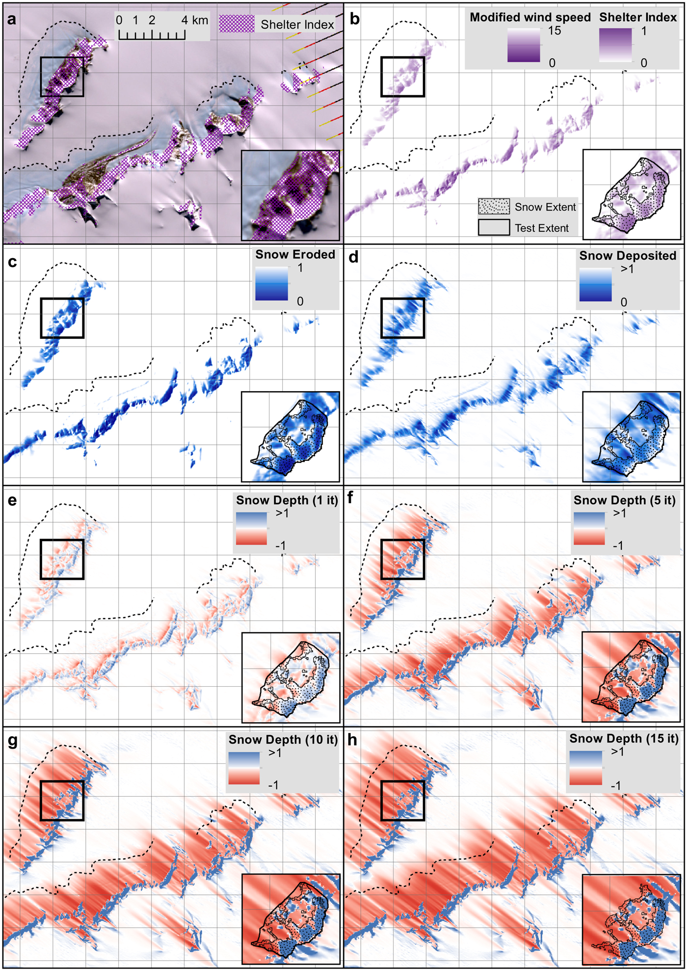
Fig. 2. Experiment 1 calculations highlight Snow_Blow outputs of (a) the Shelter index (Ti), (b) the modified wind speed (F m) and shelter index (T i), (c) snow eroded (Q e), (d) snow deposited and (e–h) the snow depth index from selected iterations (1–15), as labelled.
Table 2. Parameter sets for Snow_Blow experiment results centred on the Patriot and independence Hills (Fig. 4)

A shelter index (T i) is employed to define areas in the DEM where wind speed decreases. T i is calculated from an aspect index (A i) and slope index (S i), and these indices are described below.
4.2.1. Aspect index
A slope is assumed to be sheltered if it is within 45° of the lee aspect, where lee aspect is 180° from the dominant wind direction (Θ). The aspect index is 1 if an aspect is directly opposite to the wind direction. The aspect index is linearly scaled to 0 if the lee aspect ≥45°. This follows the suggestion by Purves and others (Reference Purves, Mackaness and Sugden1999) that the highest aspect index values lie directly in the lee of the dominant wind direction and that this decreases towards zero as the aspect of the slope approaches 45°.
4.2.2. Slope index
Following Purves and others (Reference Purves, Mackaness and Sugden1999), a slope is assumed to be sheltered if the slope is >5°. The slope index is then scaled linearly to a value of 1 (maximum shelter) at the maximum slope. The slope index (S i) is calculated in each cell as follows:


where S is the slope of the cell in question (degrees) and S max is the maximum slope angle in the DEM (degrees).
While the original Purves and others (Reference Purves, Mackaness and Sugden1999) model setup defines a minimum slope of 5°, the paper does not provide a maximum slope value, as this is derived from the maximum slope in the DEM. This approach limits the transferability of this model to other model domains with a different maximum slope, and limits the number of cells which can reach the upper end of the shelter index values. As a result, a range of S max values are employed to investigate the sensitivity of Snow_Blow outputs to changes in maximum slope, with the aim of suggesting a suitable default value. S i is capped at 1 when S max values in the DEM are greater than that set by the user.
4.2.3. Shelter index
The shelter index (T i) is then expressed as

Values of T i range from 0 (no shelter) to 1 (full shelter) (Figs 2a, b).
The modified wind speed (F m) is then calculated using the maximum wind speed (F) and the shelter index:

This produces a modified wind speed field (Fig. 2b) that is an inverse linear function of the shelter index, so is a simple parameterisation which does not take into account turbulence, or increased wind speed due to funnelling or an upslope.
4.3. Curvature index
In the original formulation of the Purves and others (Reference Purves, Mackaness and Sugden1999) shelter index (Section 4.2), the aspect calculation does not take into account the nature of the slope when it has an aspect in the lee of the wind direction. In a classic cirque morphology, for example, the curvature of the cirque would likely be concave, and, therefore, more sheltered than a slope which has a more convex curvature.
The improved model has an added option to introduce a ‘curvature index’ (C i) into the shelter index, if one is required:

where C i is a function of the plan curvature of the surface and C is the plan curvature of the cell in question:


C max is a specified maximum value at which the curvature index saturates at 1 (Supplementary Figs 4a, b). Cells with convex plan curvature (considered less sheltered) will have a positive curvature value, whereas cells with concave plan curvature (considered more sheltered) will have a negative curvature value. Although profile curvature was considered alongside plan curvature, we found that this measure could not distinguish the start of the sheltered region (e.g. the headwall of a cirque). As with S max, a user-defined value is set rather than extracting C max from the DEM.
4.4. Snow transport – erosion
Once the wind direction and speed have been adjusted, the snow transport from cell to cell can be calculated. First, the amount of snow eroded from each cell is computed. This value is dependent on the difference between the modified wind speed and the threshold wind speed. Both the Purves and others (Reference Purves, Mackaness and Sugden1999) model, and our Snow_Blow model implements a cubic relationship between the snow eroded and the proportion of the wind speed above a given threshold speed:

where Q e is the amount of snow eroded from a cell, k is a constant, F m is the modified wind speed and F t is the threshold wind speed. Although Purves and others (Reference Purves, Mackaness and Sugden1999) do not state the threshold value they use, we have selected a standard value for F t of 5 m s−1 for dry snow, following the discussion in Section 2. Values for k are not given in the Purves and others (Reference Purves, Mackaness and Sugden1999) paper. We remove the need for k by scaling the resulting erosion field from 0 (no erosion) to 1 (full erosion). Scaling the erosion also has the effect of making the absolute value of the wind speed irrelevant; instead it is the ratio of the threshold wind speed (F t) to the wind speed which is important in determining the amount of snow erosion which occurs (Fig. 3a). As a worked example, if the threshold wind speed is chosen as 5 m s−1 (as stated above) and the maximum wind speed is chosen as 15 m s−1 (blue line in Fig. 3b), this corresponds to a ratio of 1 : 3 (blue line in Fig. 3a). However, if the threshold wind speed had been chosen as 4 m s−1, and the maximum wind speed as 12 m s−1, then the erosion field would be identical, despite the maximum wind speed being lower. The full erosion value of 1, therefore, needs to be considered in the context of the ratio between the threshold wind speed and maximum wind speed, rather than the absolute value of the maximum wind speed.

Fig. 3. (a) Illustration of Eqn (7), snow erosion vs wind speed relationship. The threshold wind speed is set to 5 m s−1, therefore erosion only starts to occur once this threshold is exceeded. Maximum erosion (1) takes place once the wind speed (F) is reached. (b) Illustrates how it is the ratio between the wind speed and threshold wind speed that is important in determining the (integrated) amount of snow eroded, i.e. across the domain, less snow is eroded when the wind speed is close to the threshold wind speed. (c) Snow deposition weightings for deposition distances applied in the experiments in Table 2. (d) Number of cells with a positive snowdrift index in the test area (Fig. 2, inset) over 20 iterations.
4.5. Snow transport – deposition
Snow transport distance in the original Purves and others (Reference Purves, Mackaness and Sugden1999) model was grid dependent and snow could only be blown into one cell over a single iteration. The distance the snow was transported was therefore a function of the number of iterations used. The distance that snow can be physically transported is still a matter of debate in the literature, largely because it depends upon the method of transport (suspension vs saltation). To maintain a simplistic, accessible model these two methods of transport are grouped together to create one parameterisation in Snow_Blow.
In the Snow_Blow model, we introduce a new snow deposition routine which allows the snow deposition to follow the deflected wind direction, independently of DEM cell size. The snowdrift transport distance is modelled using an exponential distribution (see example in Fig. 3c).
Based upon this distribution's cumulative density function (i.e. 1 − eLx), the weighting (B) that governs the fraction of an origin cell's snow that ends up in a target cell is

where x 1 and x 2 are distances from the centre of the origin cell to the nearest and farthest limits of the target cell, respectively. The decay constant, L is

where md is an externally determined appropriate mean depositional distance. For computational efficiency, md sets a maximum distance that snow can be transported (mxd) as ~4.6 times md as

This explicitly accounts for 99.0% of the snow, so the weights in Eqn (8) are scaled so as to sum to 1, therefore, accounting for 100% of the snow and conserving snow mass (to within truncation error).
The mean depositional distance in Snow_Blow, and, hence, maximum distance can be modified by the user. Fetch distance in general is believed to be somewhere between 300 m (Takeuchi, Reference Takeuchi1980) and 500 m (Pomeroy and others, Reference Pomeroy, Gray and Landine1993), although larger transport distances have been reported (e.g. up to 800 m) for saltating snow grains (Braaten and Ratzlaff, Reference Braaten and Ratzlaff1998). The proportion of snow deposited decays rapidly, with the majority deposited within the first 150 m (Braaten and Ratzlaff, Reference Braaten and Ratzlaff1998). Here, we start with md as 150 m, giving an mxd of 690 m.
The eroded snow (calculated in Section 4.4) is redistributed, based on the weightings listed above using a routing algorithm designed for calculating upslope areas in hydrological modelling (Tarboton, Reference Tarboton1997). This is a recursive algorithm which uses a flow direction field to search for the upslope cells contributing to a single cell. The algorithm allows flux from one cell to travel to two of eight possible neighbouring cells (based on the Tarboton (Reference Tarboton1997) algorithm (Fig. 2d), which introduces grid-orientation dependency), which are selected based on the cells closest to the ‘flow' direction. In Snow_Blow the wind direction is substituted for flow direction so snow is redistributed according to the modified wind direction field (derived from the constant background wind input in Eqn (1)). The algorithm stores the number of contributing cells to each given cell, the proportion of snow in each cell which contributes to the given cell, and the distance of contributing cells (number of cells away), up to the maximum distance (mxd). This snow deposition weighting scheme is then applied to calculate the amount of snow that is blown into each cell (Q d).
4.6. Snow depth index
Initially, a constant and uniform snow depth of 1 is assumed. For each time step the snow depth index (h) at the end of the time step (time = t + Δt), for each cell is then calculated using the snow erosion field (Q e) and the snow deposition field (Q d) calculated above. The difference equation is

where t is the time at the start of the step and Δt is the length of the time step. Everything within the interval of t to t + Δt is assumed to be a single step (Purves and others, Reference Purves, Mackaness and Sugden1999), which means that erosion/deposition is conceptualised as instantaneous. Snow depth evolution over time may be calculated using a number of iterations.
Once the required number of iterations are completed, the snow depth index is scaled to be a difference field: areas of net loss of snow will have values of −1 ≤ h < 0, while areas of net snow gain will have positive values i.e. h > 0. Positive values can be >1 because more than one cell can contribute to the mass gain, as a result of mass loss from other cells. The results from applying different numbers of iterations of the model can be seen in Figures 2e–h. The number of cells with a positive snow depth index decreases with the number of iterations until the Snow_Blow model approaches a steady state; Figure 3d gives an example of this for the southern Heritage Range test area, shown as an inset in Figure 2. The actual amount of snow gained in the cells will continue to increase as long as there is a supply of upwind snow.
4.7. Snowdrift index
Total relative snow accumulation is dependent on the size of the cirque/catchment area. Larger cirques or catchment areas have the potential to accumulate greater amounts of snow if measured in absolute terms. In the Snow_Blow model, we follow the approach of Purves and others (Reference Purves, Mackaness and Sugden1999), to produce an output of snow depth per unit area over a catchment. This provides a more physically meaningful representation of snow accumulation. We call this the snowdrift index, which is calculated as the mean snow depth index for each gridcell across each defined catchment. We pick four, fairly contrived, sites (shown in Fig. 1b) to demonstrate the process of ‘cookie cutting’ a catchment to calculate a catchment-based snowdrift index. We choose the sites on the basis that they are sheltered from either a 122.5° or 45° wind direction, to demonstrate how the relative snowdrift index changes for each site with a different wind direction.
4.8. Boundary conditions
The user can choose whether snow is blown into the domain from outside of the domain or not. If this option is chosen, 1 unit of snow is added to every boundary gridcell. We enable this option for the purpose of our experiments. It is important to note that this introduces new snow mass into the domain at the end of every iteration in all boundary cells.
4.9. Precipitation assumption
In Snow_Blow, snow accumulation does not vary with altitude (as a result of changes in temperature) and an equal distribution of snow over the whole topography is assumed. While this is a reasonable assumption for a localised Antarctic environment, it may not be appropriate for a more temperate palaeoenvironmental setting. However, once the Snow_Blow model is run, areas below the critical threshold for solid precipitation (i.e. below the snowline) can be excluded from the analysis, if necessary.
4.10. Quantitative assessment
To compare Snow_Blow results with observed snow extent in the southernmost Ellsworth Mountains, the January 2009 Landsat image was chosen as this coincides with the meteorological data obtained for the study region (Supplementary Fig. 2). A snow/no snow mask was created on the 30 m grid for quantitative assessment. This was carried out to determine the success of each parameter set used, to provide a recommendation for the parameter choice based on the Ellsworth Mountains case study. A comparison of the observed snow/no snow areas in the January 2009 imagery (see Section 3.1) with the positive/negative values in the snow depth index, was carried out using eight iterations (see Supplementary Section 5 for more details) (Table 2). It should be noted that there is uncertainty in this process (e.g. in the georectification of the imagery, snow area classification, the various model parameters used). However, the results provide a useful measure with which to assess the suitability of each parameter set, and to identify if there is equifinality in the parameter sets. Section 5.4 shows that, in certain circumstances, the choice of parameters is not crucial, despite the uncertainty in this process.
5. Results
This section presents results from selected Snow_Blow experiments centred on the Patriot and Independence Hills in the southern Heritage Range, Antarctica, with differing model setups and parameters. We vary the depositional distance, wind speed, threshold wind speed, maximum slope angle and curvature index to determine model sensitivity to these. Table 2 gives the parameter sets used in these experiments.
5.1. Qualitative assessment
5.1.1. Areas of net snow gain
Each experiment outlined in Table 2 was run for the Heritage Range field site, to obtain a ‘best fit’ with areas of snow distribution from the Landsat imagery. A maximum deposition distance of 690 m was chosen (Expt. 1), and this was run for eight iterations (Fig. 4b). This is based on the match of the negative snow depth index predicted by Snow_Blow, and the BIA extent, mapped from the Landsat 9 January 2009 imagery (see Figs 2f, g). In this experimental output, the number of cells with a positive snow depth index continues to decrease after these eight iterations (Fig. 3d). Values <0 in Figure 4b indicate a net loss of snow, and not necessarily an absence of snow.

Fig. 4. (a) 21 September 2009 Landsat true colour composite for test area, showing mapped snow extent for model comparison. (b–f) Illustration of snow depth index at eight iterations for experiments in Table 2. (g) 21 September 2009 Landsat true colour composite for the wider study area. Dashed line indicates BIAs. (h) Snow depth index at eight iterations for Expt. 5, showing snow deposition in the lee of the mountains and erosion in the BIAs.
In the absence of snow depth measurements, a qualitative assessment of the pattern of the snow depth index against snow distribution in the January 2009 Landsat image was carried out. The initial qualitative indication is that, in general, the area of net snow gain is small relative to the snow extent of the Landsat image (Figs 4a, b show the detail of an example site). There are two potential reasons for this discrepancy, which lead to snow starvation. Firstly, the snow is not being distributed over a long enough distance downwind of an eroded cell. A longer maximum depositional distance would increase snow input to more exposed cells (see shelter index in Fig. 2b), offsetting the erosion in these cells. Due to the relatively high wind speeds in the Heritage Range, and the length of the tails seen in the imagery, there is some justification for this increased depositional distance. Secondly, the erosion may be over predicted in the model for the more exposed cells. Decreasing the amount of erosion occurring at the more exposed cells would enable the snow that is being blown into the cell to offset the erosion. Lowering the erosion in these more exposed cells can be implemented by (1) using a lower wind speed (F) relative to the threshold wind speed (see Fig. 3a), or (2) by lowering the maximum slope (S max) at which the slope index saturates at 1. We do not vary the threshold wind speed as it is the ratio between the wind speed and threshold wind speed that is important (these values are relative in the model), rather than the absolute values. It should be noted here that the maximum erosion for each cell needs to be maintained at 1 unit of snow, but that the overall erosion could be reduced.
To test the impact of increasing the maximum deposition distance, the value in the Snow_Blow model was approximately doubled from 690 to 1381 m (Expt. 2, Fig. 4c). This figure shows that an increase in the deposition distance does serve to increase the area of net snow gain in the sheltered areas, but higher deposition distances produce unrealistically long tails which are not seen in the Landsat imagery (Fig. 4a). The erosion distance is also greatly increased and a best fit to BIAs for this particular experiment is four iterations (doubling the depositional distance effectively halves the number of iterations required). The depositional area does not vary greatly between four and eight iterations; however the net snow accumulation is greater over eight iterations.
The impact of decreasing the snow erosion that occurs in the more exposed cells was tested by halving the wind speed from 15 to 7.5 m s−1 (Fig. 3a). There is a clear effect of a reduced wind speed increasing the area of net snow gain (Expt. 3, Fig. 4d). The model replicates snow accumulation in the upper parts of lee side slopes (the cirques) relatively well; however, there is less agreement in the lower areas with this lower wind speed value.
A very similar result to the above is achieved when S max is lowered (Expt. 4) by applying the default wind speed of 15 m s−1 and an S max value of 20° (for an example run) (Fig. 4e). This results in a greater agreement of snow covered areas in the lower catchment in Expt. 4, compared with Expt. 3. Despite this improvement, there remain large areas of snow accumulation in the lower parts of the valley that are not visible on the January 2009 Landsat imagery.
The curvature index was also tested in the Snow_Blow model using an F value of 15 m s−1 and an S max value of 20° (Fig. 4f). In this model run the areas of snow accumulation in the upper parts of the valley remain a good fit compared with the Landsat imagery, and the areas of snow accumulation in the lower parts (where there is limited mapped snow accumulation) are reduced, suggesting that this model run (Expt. 5) reproduces the best fit for snow accumulation.
5.1.2. Areas of net snow erosion
BIAs and snow-free areas in Horseshoe Valley indicate snow free areas created by erosion and snow starvation. The extent of the area of net snow loss depends on the number of iterations chosen, but as discussed above, eight iterations provides a snow depth index which allows a reasonable comparison with the snow free areas (Figs 4g, h). There is good general agreement in the pattern of the BIAs and areas of net snow loss, indicating that these areas are the result of a relatively simple process of snow starvation. Where the topography is more complex, e.g. in the lee of the mountains, the model produces more areas of discrepancy. While these findings imply that general trends can be simulated, with Snow_Blow, the simplicity of the shelter index and wind speed modification may not be able to fully reproduce physical processes. For example, the model does not increase the wind speed, in an area of funnelling or on an upslope which may have important consequences in specific regions, such as the areas marked ‘1’ in the example area highlighted in Fig. 4a.
Some of the observed ice-free regions in Landsat imagery, which have a positive snow depth index in the model (marked ‘2’ in Fig. 4a), are in areas where the topography is convex (see Section 4.3). The agreement in these areas is improved by incorporating the curvature index in the shelter index. A moderately high value of C max (0.5) is used in Expt. 5 (Fig. 4f). This creates a decreased area of positive snow depth index in the model output. While this mainly affects areas without observed snow, it can affect some cells with observed snow.
5.2. Quantitative assessment
The final snow depth field was compared with the observed snowfield on a pixel by pixel basis. In the model results (for the purposes of comparison) a snow depth index of <0 was considered to be ‘no snow’ and >0 as ‘snow covered’. Table 3 shows the percentage of snow predicted correctly, the percentage of ‘no snow’ predicted correctly and the overall accuracy (percentage total cells predicted correctly). The results in Table 3 show that there is a degree of equifinality in the parameter sets with a similar level of success across different parameter sets. Lower values for wind speed, F, lead to more ‘snow’ being predicted correctly, but also more snow present in the domain overall, so the ‘no snow’ areas suffer a lower level of success. Conversely, lower values of S max lead to more snow being predicted correctly, so can offset the effect of changing the wind speed. Incorporating the curvature index generally improves the prediction of no snow areas, but at a cost to the success of the prediction of snow covered areas.
Table 3. Quantitative assessment of different parameter values for F, S max and C max

Numbers in parentheses represent experiment numbers in Table 2 and Supplementary Table 1. Blue shading represents cells that predict snow/no snow most successfully, while red shading represents those predicting snow/no snow least successfully.
5.3. Snowdrift index
We derive a snowdrift index for individual catchments to determine the importance of snowdrift in relation to catchment size. These catchments were selected to reflect different orientations and presence/absence of snow cover in the Landsat imagery. The choice of values of F, S max and C max will have an impact on the absolute value of the snowdrift index for each site, and as there is no conclusive evidence to support particular values, in this section we aim to demonstrate that the choice of parameters is not critical when considering the relative snowdrift index between different sites. The combination of parameters used in Section 5.3 is used to demonstrate how the relative snowdrift index is not heavily dependent on the choice of parameters.
Sites 2 and 4 are sheltered from the 122.5° wind direction so they have a positive snowdrift index when the wind is from this direction, whereas site 1 is not sheltered from a 122.5° wind direction, so it has a negative snowdrift index (Figs 5a, b). Site 4 has a higher snowdrift index than site 2, suggesting that more snow is gained per unit area at site 4 than site 2, due to the snowdrift processes. There is no overlap in the snowdrift index with the choice of the parameters, as the degree of shelter between the sites is significantly different. However, from a 45° angle, the level of shelter is similar at sites 2 and 4 (though there is no overlap) (Figs 5c, d). The distinction between sites 1 and 3, and, 2 and 4 is still clear from this wind direction. Sites 1 and 3 are the most affected by snowdrift processes with winds from a 45° angle.
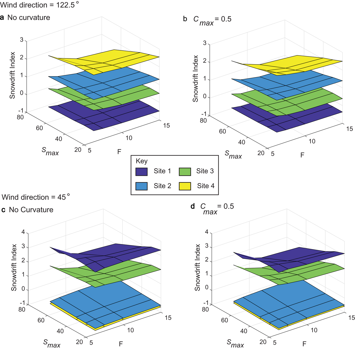
Fig. 5. Snowdrift index for sites 1–4 shown in Figure 1b for a 122.5° and 45° wind direction for various parameter sets (F = wind direction, S max is the maximum value the slope is set to for each cell, C max is the curvature index).
Once a parameter set has been chosen, the snowdrift index can be assessed for each site for various wind directions, to determine the wind direction which provides the maximum shelter for a given site and, hence, the highest snow accumulation per unit area (Fig. 6). In the case of sites 1 and 3, a ~45° wind direction would provide the most snow accumulation to these sites, though site 1 has a slightly higher value per unit area compared with site 3. In comparison, sites 2 and 4 would receive the most snow accumulation from ~135° winds, however this would be much more important at site 4 than at site 2. This is most likely due to the steeper headwall at site 4 which is able to trap more snow.

Fig. 6. Positive and negative snowdrift index for sites 1–4 shown in Figure 1b with varying wind directions, using parameter set from Expt. 5. Numbers 1–4 are the snowdrift index values.
Most of the sites also have a positive snowdrift index when the wind is coming from the opposite of the optimum direction (e.g. site 4, which has positive (although low) snowdrift index values when the wind is coming from ~330°). This output is not the result of sheltering effects, but rather, the deflection of wind, as the prevailing wind direction is re-routed by topography. Although this local deflection redistributes snow into our example sites, it also imposes an equivalent loss of snow in neighbouring areas. This process emphasises the two possible effects of snowdrift; a sheltering process and a wind driven redistribution effect.
6. Discussion
The qualitative agreement between areas of net snow gain and loss in Snow_Blow, with present day snow accumulation and snow erosion areas in Horseshoe Valley is encouraging for such a simple model. The good agreement implies that areas of snow erosion and accumulation are governed by the sheltering effect of topography in relation to the local wind flow, as opposed to regional scale wind patterns, where wind direction is constant (dominated by katabatic wind flows or funnelling). This finding is in agreement with other studies, such as that by Zwinger and others (Reference Zwinger, Malm, Schäfer, Stenberg and Moore2015). The agreement between the observed snow accumulation/erosion pattern also supports the role of snow starvation in the formation/maintenance of the BIAs in the study area.
Although the strong katabatic winds in Antarctica make our study area an extreme example of snowdrift, the Ellsworth Mountains are similar to alpine environments. Ridges in the mountain range act as a snow fence to the prevailing wind so snow is deposited within a few hundred metres of the crest, where wind speeds fall dramatically in the lee of the mountain range. With appropriate parameters, the extent of modelled snow accumulation in the lee provides excellent agreement with observed snow accumulation areas in Landsat 8 imagery. These results are therefore comparable with other polar and alpine regions, such as Greenland, where Hasholt and others (Reference Hasholt, Liston and Knudsen2003) found significant snow transport and deposition on the lee side of ridges, and in Svalbard, where Humlum (Reference Humlum2002) suggested that glacier accumulation areas coincide with areas of low wind speeds, and that glacier-free regions are usually found in exposed areas where wind speeds are high.
Snow_Blow parameterisations of snow erosion and deposition processes introduce some arbitrary choices of deposition distance and erosion parameters. However, by demonstrating that the relative snowdrift index is insensitive to these choices, we show that the impacts of these choices are minimal when the Snow_Blow model is used in a relative sense. Figure 5 demonstrates that the snow erosion formulation does have an effect on the absolute snowdrift index for individual sites. A lower ratio between wind speed and threshold wind speed leads to less erosion overall (Fig. 3a), so more snow is retained in the catchment, reflected in a higher snowdrift index value. However, this can be offset by changing the value of S max in the model.
To compare snowdrift index values across geographical areas, it would be useful to define parameters that can be used as a default set. Although independent studies are encouraged to explore the range of the sensitivity of the model to aspects such as wind speed and threshold wind speed, which can be modified to investigate the impact of varying snow conditions (such as dry and wet snow) and wind speeds. For the Heritage Range we used a representative wind speed of 15 m s−1 and a threshold wind speed of 5 m s−1 (though other wind speeds give a similar level of success). We applied an S max value of 20°, in combination with a C max value of 0.5. This provides a level of quantitative success, which is consistent across different wind speeds (Table 2). Qualitatively, an S max value of 20° improves the prediction of snow in the lower areas of the test catchment. As a result, we recommend that an S max value of 20° be adopted in future runs as a default S max value. Wind speed and threshold wind speed values can then be modified to fit the assumed wind and snow conditions for a given geographic area, e.g. a higher threshold velocity could be applied for wet snow conditions.
7. Conclusions and future work
This paper presents Snow_Blow, an improved and updated version of the Purves and others (Reference Purves, Mackaness and Sugden1999) snow redistribution model, with the addition of a flux routing algorithm, DEM resolution independence and the addition of a slope curvature component. This model was applied to a present-day environment in the Ellsworth Mountains, Antarctica, to evaluate the validity of the model for future applications, in palaeoenvironment settings. Snow_Blow reproduces patterns of snow erosion and snow deposition in Horseshoe Valley, where surface features such as snowdrift tails and wind-scoured BIAs validate model outputs. We test a variety of model parameters to define a default set for future model runs. The results show that the simplistic Snow_Blow model is suitable for palaeoenvironmental reconstructions, where meteorological observations are sparse to non-existent. It is predominantly suitable for areas with one prevailing wind direction and where sublimation is negligible, although multiple wind directions could be explored. It is also a potential tool to assess variations in snow accumulation in mountain topography throughout Antarctica, with implications for the interpretation of layers identified by radio-echo sounding (Siegert and others, Reference Siegert, Pokar, Dowdeswell and Benham2005).
The Snow_Blow model code (written in Python for easy application in ESRI ArcGIS) is freely available online at GitHub and at https://doi.org/10.5281/zenodo.3336070. While it can and should be used for a variety of purposes it is important to interrogate outputs in the context of the uncertainty of parameter values. Uncertainty is minimised when the model is used in a relative sense, for example, to compare different glacier systems. If the model is to be used in an absolute sense – for example, to apply results spatially, to account for additional precipitation onto reconstructed glacier surfaces within a mass-balance calculation – it is important to keep in mind the impact of the uncertainty in the choice of parameters on the model.
Snow_Blow could be used to calculate a snowdrift index for individual catchments (using various wind directions), to investigate how important a particular wind direction was in supplying additional mass to glaciers in palaeo settings. As additional mass will modify glacier mass balance, this type of simulation now appears critical for more robust palaeoclimatic reconstructions. Snow_Blow outputs can therefore help to explain variations in ELAs in neighbouring locations, and provide a guide as to which particular glaciers would have been the most likely representative of regional climatic conditions.
Supplementary material
The supplementary material for this article can be found at https://doi.org/10.1017/jog.2019.70
Acknowledgements
We acknowledge funding from Kingston University to EA for the initial development of the model. Project work in the southern Heritage Range was funded by the UK Natural Environment Research Council (NERC) standard grants NE/I027576/1, NE/I025840/1 and NE/I025263/1. We thank the two anonymous reviewers for their constructive comments.
Author contributions
SM conceived the idea for the model development. SM and AL wrote the manuscript with contributions from all the co-authors. KW, DS and JW provided expert input on the Ellsworth Mountains context as well as commenting on the manuscript. CB, MS and JH provided input into the background context, model methodology/experiment design as well as commenting on the manuscript. KW undertook initial model testing in the Ellsworth Mountains and analysed the wind data. AL ran the model for the study location, designed the model set-ups and parameters, and analysed the data, with advice from SM. AL produced the figures, with editing by SM. EA undertook the initial model development, supervised by MS and SM. SM and MS developed the model further and JH added the exponential distribution for snow transport. AL further developed the model and added the curvature index and snow redistributing flux algorithm.


 Open access