


1 Introduction
There is extensive evidence for the existence of filamentary structures in various plasma environments ranging from naturally occurring space plasmas to laboratory and fusion device plasmas. These non-equilibrium magnetized plasmas are often characterized by features such as filamentary density and temperature depletions or enhancements, localized currents and hot electron channels (Zweben & Medley Reference Zweben and Medley1989; Cardozo et al. Reference Cardozo, Schüller, Barth, Chu, Pijper, Lok and Oomens1994; Beurskens et al. Reference Beurskens, Lopes Cardozo, Arends, Barth and van der Meiden2001; Herranz et al. Reference Herranz, Pastor, Castejón, de la Luna, García-Cortés, Barth, Ascasíbar, Sánchez and Tribaldos2000). From detailed measurements in the laboratory and by satellites, these structures are associated with turbulent fluctuations that are spontaneously generated through free energy sources such as gradients in their macroscopic plasma parameters (Stasiewciz et al. Reference Stasiewciz, Gustafsson, Marklund, Lindqvist, Clemmons and Zanetti1997; Morales et al. Reference Morales, Maggs, Burke and Peñano1999; Burke, Maggs & Morales Reference Burke, Maggs and Morales2000c ; Wygant et al. Reference Wygant, Keiling, Cattell, Johnson, Lysak, Temerin, Mozer, Kletzing, Scudder and Peterson2000). The properties of turbulence appearing in such structures are particularly relevant to the plasma edge region of magnetic confinement devices where large fluctuation bursts and cross-field blob and filament transport are connected with nonlinear interactions of Alfvénic fluctuations (Serianni et al. Reference Serianni, Agostini, Antoni, Cavazzana, Martines, Sattin, Scarin, Spada, Spolaore and Vianello2007).
The transverse scale of filamentary plasma structures can vary widely, from the collisionless electron skin depth to several times the ion Larmor radius, depending on the parameter ordering. Plasma non-uniformities on these scales can induce low frequency excitations such as drift-Alfvén waves and vortices (Abdalla et al. Reference Abdalla, Kuvshinov, Schep and Westerhof2001). These wave modes have previously been investigated under controlled conditions using a single isolated heat source embedded in a large linear plasma device (Burke, Maggs & Morales Reference Burke, Maggs and Morales1998, Reference Burke, Maggs and Morales2000a ,Reference Burke, Maggs and Morales b ,Reference Burke, Maggs and Morales c ; Pace et al. Reference Pace, Shi, Maggs, Morales and Carter2008a ,Reference Pace, Shi, Maggs, Morales and Carter b ,Reference Pace, Shi, Maggs, Morales and Carter c ; Karbashewski et al. Reference Karbashewski, Sydora, Van Compernolle and Poulos2018). In these experiments a low-voltage electron beam was injected into a strongly magnetized, cold, afterglow plasma. This produced a long (∼8 m) and narrow (∼10 mm diameter) filament of elevated temperature (∼20 times the background), isolated from the walls of the chamber (0.6 m diameter). The experiments established that there is a transition from a period of classical transport (Burke et al. Reference Burke, Maggs and Morales2000a ) (due to Coulomb collisions) to one of anomalous transport (Burke et al. Reference Burke, Maggs and Morales2000b ). In this latter phase, localized drift-Alfvén eigenmodes were driven unstable by the temperature gradient in the filament edge. As the plasma conditions changed the highly coherent eigenmodes evolved into broadband drift-Alfvénic turbulence (Pace et al. Reference Pace, Shi, Maggs, Morales and Carter2008a ,Reference Pace, Shi, Maggs, Morales and Carter b ).
The experiments motivated numerical modelling studies of
 $\boldsymbol{E}\times \boldsymbol{B}$
advection in the potential fields of low frequency drift waves (Shi et al.
Reference Shi, Pace, Morales, Maggs and Carter2009), where
$\boldsymbol{E}\times \boldsymbol{B}$
advection in the potential fields of low frequency drift waves (Shi et al.
Reference Shi, Pace, Morales, Maggs and Carter2009), where
 $\boldsymbol{E}$
is the electric field and
$\boldsymbol{E}$
is the electric field and
 $\boldsymbol{B}$
the magnetic field. It was found that, above a certain threshold amplitude, the interaction of spatially and temporally coherent drift waves resulted in chaotic Lagrangian orbits. The temporal signal of the temperature fluctuations constructed from these orbits consists of Lorentzian-shaped pulses which have a frequency spectrum that is exponential and consistent with diagnostic probe measurements (Pace et al.
Reference Pace, Shi, Maggs, Morales and Carter2008a
,Reference Pace, Shi, Maggs, Morales and Carter
b
; Maggs & Morales Reference Maggs and Morales2013). This study was followed by three-dimensional gyrokinetic simulations of cross-field transport driven by drift-Alfvén waves in a single magnetized temperature filament (Sydora et al.
Reference Sydora, Morales, Maggs and Van Compernolle2015). The simulations demonstrated the excitation of convective cells from nonlinear drift-Alfvén mode interactions and enhanced cross-field transport through strongly nonlinear
$\boldsymbol{B}$
the magnetic field. It was found that, above a certain threshold amplitude, the interaction of spatially and temporally coherent drift waves resulted in chaotic Lagrangian orbits. The temporal signal of the temperature fluctuations constructed from these orbits consists of Lorentzian-shaped pulses which have a frequency spectrum that is exponential and consistent with diagnostic probe measurements (Pace et al.
Reference Pace, Shi, Maggs, Morales and Carter2008a
,Reference Pace, Shi, Maggs, Morales and Carter
b
; Maggs & Morales Reference Maggs and Morales2013). This study was followed by three-dimensional gyrokinetic simulations of cross-field transport driven by drift-Alfvén waves in a single magnetized temperature filament (Sydora et al.
Reference Sydora, Morales, Maggs and Van Compernolle2015). The simulations demonstrated the excitation of convective cells from nonlinear drift-Alfvén mode interactions and enhanced cross-field transport through strongly nonlinear
 $\boldsymbol{E}\times \boldsymbol{B}$
advection in the filament.
$\boldsymbol{E}\times \boldsymbol{B}$
advection in the filament.
Since filamentary structures are generally not isolated but may occur in bundles, the present study considers the interaction of multiple filamentary structures in close proximity. Therefore, we extend previous laboratory experiments made with single magnetized thermal filaments to regimes of enhanced cross-field transport arising from filament–filament interactions. We have found that when the filaments are sufficiently close the drift-Alfvén eigenmodes forming on individual filaments overlap and through rapid profile changes, spontaneously generate near azimuthally symmetric drift-Alfvén modes with maximum amplitude peaked towards the edge of the bundle where thermal gradients are steep.
The paper is organized as follows: § 2 presents the experiment set-up and parameters followed by a presentation of the experiment results in § 3. In § 4 an emissive cathode model is used to predict the radial plasma potential profile and resultant azimuthal flow profile that is incorporated in the drift-Alfvén stability analysis. The linear eigenmode stability and predicted mode structure are given in § 5 using the thermal and azimuthal flow profiles taken from experiment. Section 6 is a discussion of the results and § 7 gives the summary.
2 Experiment set-up
The experiment is performed on the upgraded large plasma device (LAPD) (Gekelman et al. Reference Gekelman, Pribyl, Lucky, Drandell, Leneman, Maggs, Vincena, Van Compernolle, Tripathi and Morales2016) operated by the basic plasma science facility at the University of California, Los Angeles. A schematic, not to scale, is shown in figure 1(a). The LAPD is a cylindrical device, with an axial magnetic field that confines a quiescent plasma column 18 m long and 60 cm in diameter. The plasma is created from collisional ionization of He gas by 70 eV electrons of a large area low-voltage electron beam, produced by the application of a positive voltage between a barium oxide (BaO) coated cathode and a mesh anode 50 cm away. The electron beam heats the plasma to electron temperatures in the range of 5 eV. The active phase lasts for 12 ms and is repeated every second (1 Hz pulse rate). The magnetic field in the experiment is uniform and is set to 1000 G.
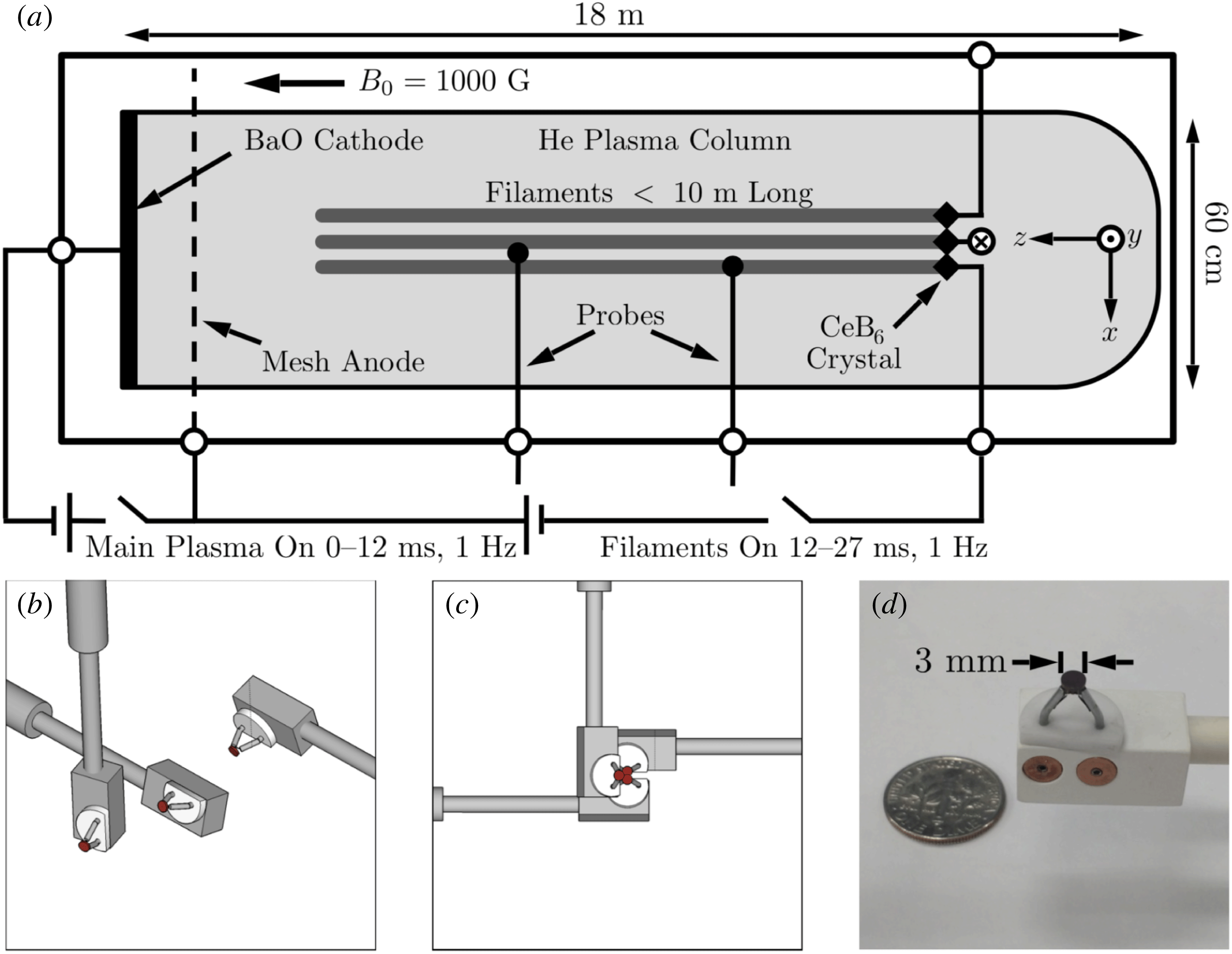
Figure 1. (a) Schematic of the experiment set-up on the LAPD (not to scale). The probes with crystal cathodes on the end are inserted through ports on the east, west and top of the plasma chamber. (b) View of the cathode probes from an angle showing the axial offset and angling of the tips. (c) A
 $z$
-axis view of the crystals in the closest configuration. (d) Image of one of the CeB6 crystals mounted on a probe next to an American dime for scale reference.
$z$
-axis view of the crystals in the closest configuration. (d) Image of one of the CeB6 crystals mounted on a probe next to an American dime for scale reference.
In the experiment three cerium hexaboride (CeB6) crystals are introduced on the opposite side of the LAPD vacuum vessel, as shown in figure 1(a). CeB6 is a refractory ceramic material and is stable in vacuum. It has a low work function, and one of the highest electron emissivities known when heated to its operating temperature in the range of 1400° C. When the CeB6 crystals are biased with respect to an axially distant anode 15 m away, electrons are emitted from the CeB6 along field lines connected to the CeB6 crystals. This results in three heated filaments, each a few mm in diameter but several metres long. The discharge voltage applied between the CeB6 crystals and the distant anode is kept below the ionization potential for the Helium fill gas, i.e. ⩽25 V. Each crystal has its own discharge pulsing circuit, such that the discharge bias and timing can be different for each crystal.
The experiment is performed during the afterglow phase, after the active phase of the LAPD discharge is terminated. In the afterglow phase, the 70 eV beam from the BaO cathode is turned off, and the electron temperature falls below 0.5 eV within 100 μs while the plasma density decreases on a time scale of tens of milliseconds. An example of the time evolution of the electron density,
 $n_{e}$
, and temperature,
$n_{e}$
, and temperature,
 $T_{e}$
, in the afterglow phase is shown in figure 2 in the absence of heating by the CeB6 crystals. The shaded regions indicate the time during which the CeB6 thermionic emitter is active, i.e. biased negative with respect to the anode. The heating pulse typically lasts for 10–20 ms. The start of the heating pulse is taken as
$T_{e}$
, in the afterglow phase is shown in figure 2 in the absence of heating by the CeB6 crystals. The shaded regions indicate the time during which the CeB6 thermionic emitter is active, i.e. biased negative with respect to the anode. The heating pulse typically lasts for 10–20 ms. The start of the heating pulse is taken as
 $t=0$
and the axial location of the CeB6 cathode as
$t=0$
and the axial location of the CeB6 cathode as
 $z=0$
.
$z=0$
.
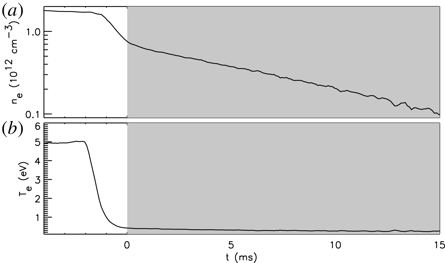
Figure 2. Typical temporal evolution of (a) electron density shown in log scale and (b) electron temperature in LAPD in the absence of heating by the CeB6 crystals. Shaded regions indicate when the thermionic emitter is actively biased.
The three CeB6 crystals were purchased from Applied Physics Technologies (APT 2019, http://www.a-p-tech.com/). The crystals are held by two current carrying rigid wires, which in turn are mounted on a ceramic base. The disk-shaped ceramic bases were slightly modified as shown in figure 1(b–d), and are being held by a boron nitride rectangular prism mounted on a probe shaft. The electrical connections between insulated wires inside the probe shaft and the current carrying rigid wires holding the CeB6 crystals are done inside the boron nitride prisms. The mounting structures and probe shaft geometry were designed such that the CeB6 crystals can be positioned arbitrarily close to each other when viewed along the magnetic field line (
 $z$
-axis), as shown in figure 1(c). In order to achieve this, the crystals are set back by a few cm in the
$z$
-axis), as shown in figure 1(c). In order to achieve this, the crystals are set back by a few cm in the
 $z$
-direction (figure 1
b). From the position shown in figure 1(c) the crystals can be separated to any inter-crystal distance required by the experiment.
$z$
-direction (figure 1
b). From the position shown in figure 1(c) the crystals can be separated to any inter-crystal distance required by the experiment.
The properties of the LAPD plasmas are sampled with probes through vacuum ports spaced every 32 cm along the axial direction (
 $z$
-axis) of the cylindrical vacuum chamber. Probes are inserted into the vacuum chamber through ball valves (Leneman & Gekelman Reference Leneman and Gekelman2001) which allow for three-dimensional movement. Probes are mounted on an external probe drive system and can be moved to a prescribed position with sub-millimetre accuracy. The data acquisition system is fully automated; it controls the digitizers and the probe drive system. Typically, a probe moves through a series of user defined (
$z$
-axis) of the cylindrical vacuum chamber. Probes are inserted into the vacuum chamber through ball valves (Leneman & Gekelman Reference Leneman and Gekelman2001) which allow for three-dimensional movement. Probes are mounted on an external probe drive system and can be moved to a prescribed position with sub-millimetre accuracy. The data acquisition system is fully automated; it controls the digitizers and the probe drive system. Typically, a probe moves through a series of user defined (
 $x,y$
) transverse positions at a fixed axial position,
$x,y$
) transverse positions at a fixed axial position,
 $z$
. At each position, data from several plasma pulses are acquired and stored, before moving to the next position. Since the LAPD plasma is highly reproducible, an ensemble measurement of the plasma parameters can thus be obtained. The main set of probe diagnostics in this experiment sample the ion saturation current, both the mean evolution and the fluctuating part. Other measurements include plasma potential, electron temperature and density. Information about these quantities is obtained from the I-V characteristic of a swept Langmuir probe. Additionally, transverse magnetic fluctuations,
$z$
. At each position, data from several plasma pulses are acquired and stored, before moving to the next position. Since the LAPD plasma is highly reproducible, an ensemble measurement of the plasma parameters can thus be obtained. The main set of probe diagnostics in this experiment sample the ion saturation current, both the mean evolution and the fluctuating part. Other measurements include plasma potential, electron temperature and density. Information about these quantities is obtained from the I-V characteristic of a swept Langmuir probe. Additionally, transverse magnetic fluctuations,
 $\unicode[STIX]{x1D6FF}\boldsymbol{B}_{\bot }$
, are measured using probes with
$\unicode[STIX]{x1D6FF}\boldsymbol{B}_{\bot }$
, are measured using probes with
 $\text{d}\boldsymbol{B}/\text{d}t$
loops.
$\text{d}\boldsymbol{B}/\text{d}t$
loops.
3 Experiment results
Two different inter-crystal distances are presented here; a close separation where the distance of the cathodes from a central origin is adjusted to be ∼5 mm, and a far separation where the distance from the origin is ∼15 mm. For the far separation, the discharge bias on each cathode is equal at 15 V, resulting in nearly identical plasma discharge currents for each crystal. In the close separation, equal biases on each cathode resulted in different discharge currents due to a shadowing effect by the forward cathodes on those staggered to the rear (figure 1 b). To remedy the uneven beam power, voltages of 11, 16 and 20 V were used for the front, middle and rear crystals, respectively; figure 3 shows the beam power over time for the close separation configuration. It is clear that in adjusting the voltages a nearly uniform beam power was achieved across each of the cathodes. Performing this power matching step is necessary to ensure similar heating of the plasma from each cathode.

Figure 3. Beam power for each CeB6 crystal cathode when in the close separation configuration.
Figure 4 shows probe measurements in a transverse plane located at
 $z=290~\text{cm}$
from the cathode sources, taken shortly after the cathode bias is applied (∼0.1 ms). In each of the panels, dual scale
$z=290~\text{cm}$
from the cathode sources, taken shortly after the cathode bias is applied (∼0.1 ms). In each of the panels, dual scale
 $x{-}y$
axes are used for the dimensions of the plane. The lower and left axes are in centimetres while the upper and right axes are in normalized units; we use the electron skin depth scale,
$x{-}y$
axes are used for the dimensions of the plane. The lower and left axes are in centimetres while the upper and right axes are in normalized units; we use the electron skin depth scale,
 $\unicode[STIX]{x1D6FF}_{e}$
, computed using the density of 1012 cm-3. Figure 4(a) is a plane of ion saturation current for the far separation and shows the filaments each maintain a distinct structure but develop convective tails, indicating interaction between the filaments. Figure 4(b) shows the same plane of fluctuations in the ion saturation current,
$\unicode[STIX]{x1D6FF}_{e}$
, computed using the density of 1012 cm-3. Figure 4(a) is a plane of ion saturation current for the far separation and shows the filaments each maintain a distinct structure but develop convective tails, indicating interaction between the filaments. Figure 4(b) shows the same plane of fluctuations in the ion saturation current,
 $\unicode[STIX]{x1D6FF}I_{\text{sat}}$
, bandpass filtered around 25 kHz (5 kHz width). There is evidence of distinct mode structures on each of the filaments with fluctuation levels around
$\unicode[STIX]{x1D6FF}I_{\text{sat}}$
, bandpass filtered around 25 kHz (5 kHz width). There is evidence of distinct mode structures on each of the filaments with fluctuation levels around
 $\unicode[STIX]{x1D6FF}I_{\text{sat}}/I_{\text{sat}}\approx 20\,\%$
, with lower fluctuation levels between the filaments (
$\unicode[STIX]{x1D6FF}I_{\text{sat}}/I_{\text{sat}}\approx 20\,\%$
, with lower fluctuation levels between the filaments (
 $\unicode[STIX]{x1D6FF}I_{\text{sat}}/I_{\text{sat}}\approx ~5{-}10\,\%$
). The frequency of 25 kHz and similarity in structure to previous single filament experiments indicates that each filament rapidly develops drift-Alfvén wave fluctuations (Burke et al.
Reference Burke, Maggs and Morales2000b
; Pace et al.
Reference Pace, Shi, Maggs, Morales and Carter2008a
). The formation of the tails may be due to transverse
$\unicode[STIX]{x1D6FF}I_{\text{sat}}/I_{\text{sat}}\approx ~5{-}10\,\%$
). The frequency of 25 kHz and similarity in structure to previous single filament experiments indicates that each filament rapidly develops drift-Alfvén wave fluctuations (Burke et al.
Reference Burke, Maggs and Morales2000b
; Pace et al.
Reference Pace, Shi, Maggs, Morales and Carter2008a
). The formation of the tails may be due to transverse
 $\boldsymbol{E}\times \boldsymbol{B}$
flows generated by radial electric fields directed toward the centre of each filament or through enhanced cross-field transport due to interaction between the drift-Alfvén modes.
$\boldsymbol{E}\times \boldsymbol{B}$
flows generated by radial electric fields directed toward the centre of each filament or through enhanced cross-field transport due to interaction between the drift-Alfvén modes.

Figure 4. Probe measurements for different arrangements of the filaments just after turning on,
 $t=0.1~\text{ms}$
. (a)
$t=0.1~\text{ms}$
. (a)
 $I_{\text{sat}}$
for the filaments in far proximity. (b) Filtered fluctuation levels in (a) at ∼25 kHz. (c) Filtered fluctuation levels in (a) below 5 kHz. (d)
$I_{\text{sat}}$
for the filaments in far proximity. (b) Filtered fluctuation levels in (a) at ∼25 kHz. (c) Filtered fluctuation levels in (a) below 5 kHz. (d)
 $I_{\text{sat}}$
when the filaments are positioned close together. (e) Filtered fluctuation levels for (d) at ∼20 kHz. (f) Filtered fluctuation levels for (d) below 5 kHz. (g) Unfiltered magnetic fluctuations,
$I_{\text{sat}}$
when the filaments are positioned close together. (e) Filtered fluctuation levels for (d) at ∼20 kHz. (f) Filtered fluctuation levels for (d) below 5 kHz. (g) Unfiltered magnetic fluctuations,
 $\unicode[STIX]{x1D6FF}\boldsymbol{B}_{\bot }$
, showing a dipole rotating at ∼25 kHz.
$\unicode[STIX]{x1D6FF}\boldsymbol{B}_{\bot }$
, showing a dipole rotating at ∼25 kHz.
In the close separation, all three filaments have appeared by 0.1 ms (figure 4
d). The filaments are initially highly active spatially and distorted before settling into stable positions in a triangular configuration with overlapping gradients by ∼0.5 ms. Prior to the appearance of all three filaments, by 0.1 ms there is first only a single filamentary structure that eventually settles in position of the front cathode (bottom left); fluctuations in ion saturation current show a strong (
 $\unicode[STIX]{x1D6FF}I_{\text{sat}}/I_{\text{sat}}\approx 30\,\%$
)
$\unicode[STIX]{x1D6FF}I_{\text{sat}}/I_{\text{sat}}\approx 30\,\%$
)
 $m=1$
fluctuation around this single filament at ∼25 kHz, indicating that prior to the set up of the other two filaments this single filament is behaving as a mostly independent filament like the separated filaments in figure 4(a) and previous single filament experiments. A plane of
$m=1$
fluctuation around this single filament at ∼25 kHz, indicating that prior to the set up of the other two filaments this single filament is behaving as a mostly independent filament like the separated filaments in figure 4(a) and previous single filament experiments. A plane of
 $\unicode[STIX]{x1D6FF}I_{\text{sat}}$
at
$\unicode[STIX]{x1D6FF}I_{\text{sat}}$
at
 $t=0.1~\text{ms}$
and bandpass filtered around 20 kHz (5 kHz width) is shown in figure 4(e). The 20 kHz fluctuations show a pattern with an
$t=0.1~\text{ms}$
and bandpass filtered around 20 kHz (5 kHz width) is shown in figure 4(e). The 20 kHz fluctuations show a pattern with an
 $m=3$
azimuthal mode number rotating in the direction of the electron diamagnetic drift (counter-clockwise in figure 4
e). The structure appears to be a global mode centred on all three filaments that persists throughout the discharge and will be analysed further in this manuscript.
$m=3$
azimuthal mode number rotating in the direction of the electron diamagnetic drift (counter-clockwise in figure 4
e). The structure appears to be a global mode centred on all three filaments that persists throughout the discharge and will be analysed further in this manuscript.
Figure 4(g) shows unfiltered magnetic fluctuations (
 $\unicode[STIX]{x1D6FF}\boldsymbol{B}_{\bot }<0.5~\text{mG}$
) that indicate a dipole structure that rotates at a frequency of 25 kHz. A similar magnetic structure was observed in the single filament case in conjunction with an
$\unicode[STIX]{x1D6FF}\boldsymbol{B}_{\bot }<0.5~\text{mG}$
) that indicate a dipole structure that rotates at a frequency of 25 kHz. A similar magnetic structure was observed in the single filament case in conjunction with an
 $m=1$
drift-Alfvén wave and physically represents two opposing current channels in the axial direction that rotate around the filament structure (Burke et al.
Reference Burke, Maggs and Morales2000b
). Of particular interest is that the dipole is centred on the bottom left filament, the front-most cathode, which initially shows the strongest heating and the frequency matches the frequency of the drift-Alfvén waves observed on the separated filaments (figure 4
b) and the initial
$m=1$
drift-Alfvén wave and physically represents two opposing current channels in the axial direction that rotate around the filament structure (Burke et al.
Reference Burke, Maggs and Morales2000b
). Of particular interest is that the dipole is centred on the bottom left filament, the front-most cathode, which initially shows the strongest heating and the frequency matches the frequency of the drift-Alfvén waves observed on the separated filaments (figure 4
b) and the initial
 $m=1$
structure before the two other filaments appear. Beyond ∼0.1 ms the magnetic dipole like structure develops a less dominant but more complex magnetic structure with evidence of several more alternating current channels with a rotation centred on the full tri-filament structure at a slightly lower frequency of ∼20 kHz, the same as the
$m=1$
structure before the two other filaments appear. Beyond ∼0.1 ms the magnetic dipole like structure develops a less dominant but more complex magnetic structure with evidence of several more alternating current channels with a rotation centred on the full tri-filament structure at a slightly lower frequency of ∼20 kHz, the same as the
 $m=3$
pattern in figure 4(b). This situation during the initial turn on can be interpreted as the bottom left filament developing a drift-Alfvén wave independent of the other two filaments and then the heated region from all three filaments develops the
$m=3$
pattern in figure 4(b). This situation during the initial turn on can be interpreted as the bottom left filament developing a drift-Alfvén wave independent of the other two filaments and then the heated region from all three filaments develops the
 $m=3$
mode with magnetic fluctuations of a lower magnitude than the dipole structure from the
$m=3$
mode with magnetic fluctuations of a lower magnitude than the dipole structure from the
 $m=1$
mode.
$m=1$
mode.
In addition to the drift-Alfvén fluctuations that appear shortly after the bias is applied, there are short lived, low frequency (<5 kHz) fluctuations in a tornado-like spiral pattern with a radial extent of several centimetres – similar to those seen in a ring-shaped cathode experiment in the LAPD (Poulos, Van Compernolle & Morales Reference Poulos, Van Compernolle and Morales2017). This is shown in figures 4(c) and 4(f) where
 $\unicode[STIX]{x1D6FF}I_{\text{sat}}$
is low-pass filtered below 5 kHz; note that the size of the planes are larger than in figure 4(a,b) and (d,e), respectively, and that the spiral arms clearly extend beyond the full data collection plane indicating extensive cross-field transport well beyond the heated region with fluctuation levels of ∼10 %; in contrast, the ring-shaped cathode experiment observed fluctuations of the order of ∼30 %. It has been suggested (Poulos et al.
Reference Poulos, Van Compernolle and Morales2017) that the tornado-like mode is due to vorticity in the plasma generated by the emissive cathode boundaries. The tornado structure in the far separation case (figure 4
c) initially shows tornado-like development around each filament and progresses to a structure surrounding all three filaments; in contrast, the close separation case (figure 4
f) shows a single tornado structure developing around the bundle. It should be noted that while the tornado structure has significant radial extent and it is reasonable to wonder if it may be a characteristic of the afterglow plasma, it is not present in discharges until the bias is applied to the crystal cathodes and the individual arms around the separated filaments indicate it clearly develops from the emissive cathodes. In this manuscript, the main focus is on an analysis of the close separation configuration once the filaments reach a stable configuration, i.e. beyond ∼0.5 ms where the transient tornado-like mode is not present.
$\unicode[STIX]{x1D6FF}I_{\text{sat}}$
is low-pass filtered below 5 kHz; note that the size of the planes are larger than in figure 4(a,b) and (d,e), respectively, and that the spiral arms clearly extend beyond the full data collection plane indicating extensive cross-field transport well beyond the heated region with fluctuation levels of ∼10 %; in contrast, the ring-shaped cathode experiment observed fluctuations of the order of ∼30 %. It has been suggested (Poulos et al.
Reference Poulos, Van Compernolle and Morales2017) that the tornado-like mode is due to vorticity in the plasma generated by the emissive cathode boundaries. The tornado structure in the far separation case (figure 4
c) initially shows tornado-like development around each filament and progresses to a structure surrounding all three filaments; in contrast, the close separation case (figure 4
f) shows a single tornado structure developing around the bundle. It should be noted that while the tornado structure has significant radial extent and it is reasonable to wonder if it may be a characteristic of the afterglow plasma, it is not present in discharges until the bias is applied to the crystal cathodes and the individual arms around the separated filaments indicate it clearly develops from the emissive cathodes. In this manuscript, the main focus is on an analysis of the close separation configuration once the filaments reach a stable configuration, i.e. beyond ∼0.5 ms where the transient tornado-like mode is not present.
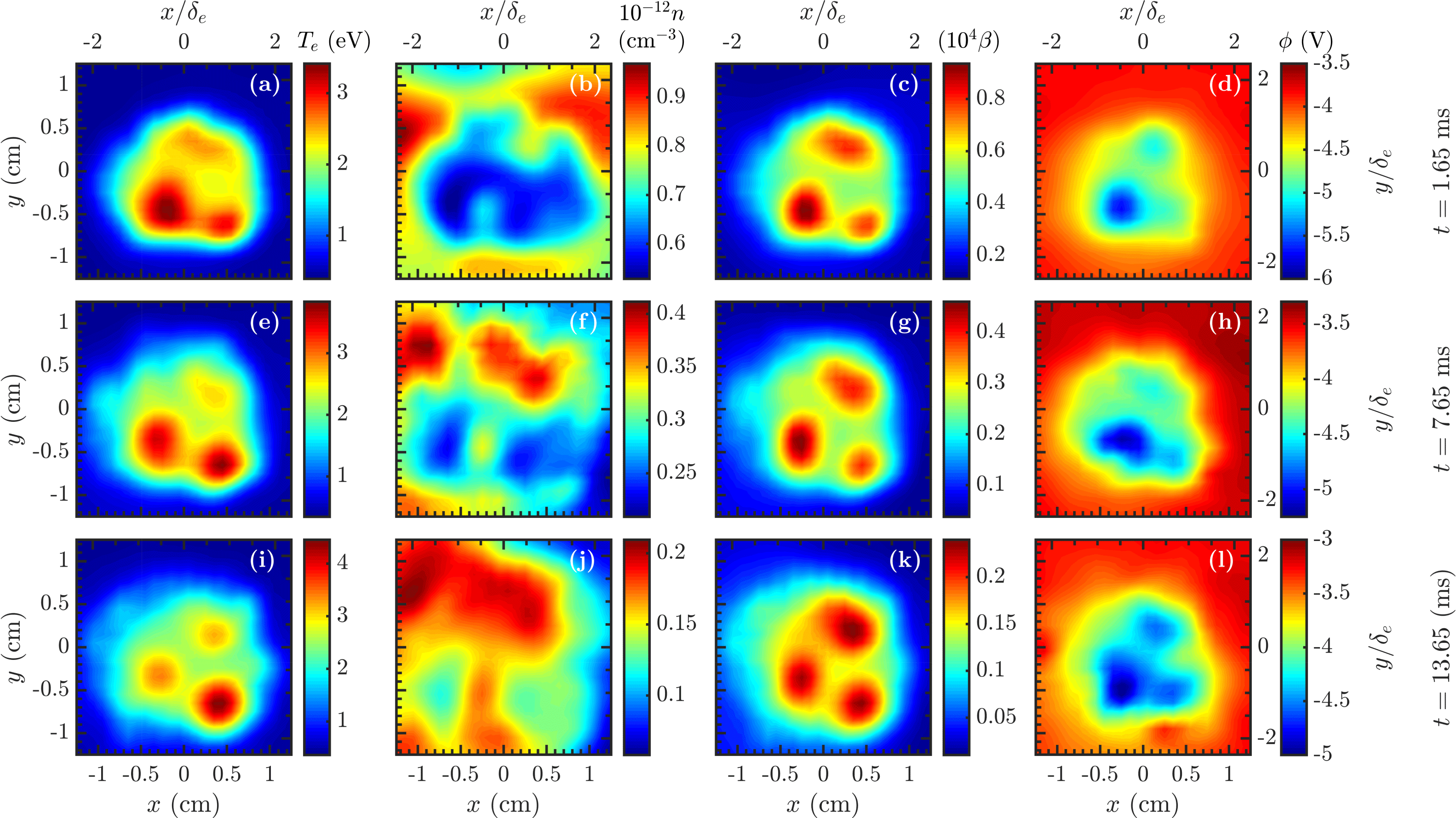
Figure 5. Temperature (a,e,i), density (b,f,j), electron plasma beta (c,g,k) and space (plasma) potential (d,h,l) for three different times during the evolution of the 3 filament structure. The data were acquired using rapidly swept Langmuir probes at a distance
 $z=290~\text{cm}$
from the most forward source.
$z=290~\text{cm}$
from the most forward source.
The electron temperature,
 $T_{e}$
, density,
$T_{e}$
, density,
 $n$
, and space (plasma) potential,
$n$
, and space (plasma) potential,
 $\unicode[STIX]{x1D719}$
, can be determined by rapidly sweeping (400 μs) the probe bias to collect characteristic Langmuir I–V curves. A standard analysis of the I–V curves yields the parameters of interest (Chen Reference Chen2001; Merlino Reference Merlino2007). While this method does not deliver high time resolution and has an element of uncertainty due to fluctuations in the parameters during the sweep, a long term evolution of the parameters can be determined. Figure 5 shows planes of,
$\unicode[STIX]{x1D719}$
, can be determined by rapidly sweeping (400 μs) the probe bias to collect characteristic Langmuir I–V curves. A standard analysis of the I–V curves yields the parameters of interest (Chen Reference Chen2001; Merlino Reference Merlino2007). While this method does not deliver high time resolution and has an element of uncertainty due to fluctuations in the parameters during the sweep, a long term evolution of the parameters can be determined. Figure 5 shows planes of,
 $T_{e}$
,
$T_{e}$
,
 $n$
,
$n$
,
 $\unicode[STIX]{x1D6FD}$
and
$\unicode[STIX]{x1D6FD}$
and
 $\unicode[STIX]{x1D719}$
for
$\unicode[STIX]{x1D719}$
for
 $t=1.65$
, 7.65 and 13.65 ms, highlighting the start, middle and end of a 15 ms discharge when the filaments are in the close separation. Here, the electron plasma
$t=1.65$
, 7.65 and 13.65 ms, highlighting the start, middle and end of a 15 ms discharge when the filaments are in the close separation. Here, the electron plasma
 $\unicode[STIX]{x1D6FD}$
is determined using
$\unicode[STIX]{x1D6FD}$
is determined using
 $\unicode[STIX]{x1D6FD}=8\unicode[STIX]{x03C0}n_{e}T_{e}/B_{o}^{2}$
and is proportional to the electron plasma pressure. Initially, the density is slightly non-uniform with a decrease in the regions of highest temperature; this is in stark contrast to previously documented single filament behaviour that shows enhanced density in the centre of the filament (Karbashewski et al.
Reference Karbashewski, Sydora, Van Compernolle and Poulos2018). By the middle of the discharge any large spatial differences in density have disappeared and by the end of the experiment the variations in density are minimal (note the range of the colour bar). Recall that the background density decays substantially during this time frame due to plasma outflows to the axial ends of the machine.
$\unicode[STIX]{x1D6FD}=8\unicode[STIX]{x03C0}n_{e}T_{e}/B_{o}^{2}$
and is proportional to the electron plasma pressure. Initially, the density is slightly non-uniform with a decrease in the regions of highest temperature; this is in stark contrast to previously documented single filament behaviour that shows enhanced density in the centre of the filament (Karbashewski et al.
Reference Karbashewski, Sydora, Van Compernolle and Poulos2018). By the middle of the discharge any large spatial differences in density have disappeared and by the end of the experiment the variations in density are minimal (note the range of the colour bar). Recall that the background density decays substantially during this time frame due to plasma outflows to the axial ends of the machine.
The locations of the temperature filaments remain stationary and the filaments become more uniform as the experiment progresses. The temperature of the filaments increases from approximately 3 eV to approximately 4 eV. The pressure profile remains largely unchanged qualitatively, and is similar to the temperature. The absolute pressure is dropping due to the continued decrease of plasma density throughout the experiment. The space potential forms a well where the cathodes are located, as expected from similar experiments (Van Compernolle & Morales Reference Van Compernolle and Morales2017; Jin et al. Reference Jin, Poulos, Van Compernolle and Morales2019), but has a noticeable asymmetry in the magnitude with the bottom left filament having a significantly lower space potential in figure 5(d). Referring to figure 1(b,c), the bottom left cathode is the front most cathode and it is likely the probe and crystal are shadowing the potential from the other cathodes. Towards the end of the experiment, this shadowing effect is reduced. In all of the temperatures, pressures and potentials the individual filament gradients are overlapped and produce a global gradient structure around the tri-filament bundle.

Figure 6. (a) Time series of
 $\unicode[STIX]{x1D6FF}I_{\text{sat}}$
for a single shot at a radius of
$\unicode[STIX]{x1D6FF}I_{\text{sat}}$
for a single shot at a radius of
 $r=1~\text{cm}$
from the approximate centre of the close separation triangular filament configuration. (b) Ensemble average of the power spectra of the shaded region in (a) for all shots with a radius of
$r=1~\text{cm}$
from the approximate centre of the close separation triangular filament configuration. (b) Ensemble average of the power spectra of the shaded region in (a) for all shots with a radius of
 $r=1~\text{cm}$
from the moving probe (black) and the reference probe at a stationary position on the outer gradient (red). (c) Power spectrum of a single shot (panel a) demonstrating the exponential decay of the power spectrum. (d) Time series of
$r=1~\text{cm}$
from the moving probe (black) and the reference probe at a stationary position on the outer gradient (red). (c) Power spectrum of a single shot (panel a) demonstrating the exponential decay of the power spectrum. (d) Time series of
 $\unicode[STIX]{x1D6FF}I_{\text{sat}}$
for a single shot at a radius of
$\unicode[STIX]{x1D6FF}I_{\text{sat}}$
for a single shot at a radius of
 $r=0.3~\text{cm}$
from the approximate centre of the top right filament in the far separation configuration. (c) Power spectrum of a single shot (panel d) similar to previously reported single filament spectra, establishing the filaments behave mostly independently in the far separation.
$r=0.3~\text{cm}$
from the approximate centre of the top right filament in the far separation configuration. (c) Power spectrum of a single shot (panel d) similar to previously reported single filament spectra, establishing the filaments behave mostly independently in the far separation.
Figure 6(a) shows a time trace for single shot of fluctuations in ion saturation current collected on the outer gradient of the tri-filament bundle. The fluctuations are broadband with very little evidence of coherent wave activity and the shot has a high degree of temporal uniformity. This temporal consistency is in contrast to the single filament situation where the filament transitions through several different transport regimes with fluctuations exhibiting a coherent phase followed by steady broadband perturbations (Burke et al.
Reference Burke, Maggs and Morales2000a
,Reference Burke, Maggs and Morales
b
; Pace et al.
Reference Pace, Shi, Maggs, Morales and Carter2008a
). A frequency analysis of the 3 ms long shaded region in figure 6(a) is shown in figure 6(b) for an ensemble of plasma shots all falling at a radius of
 $r=1~\text{cm}$
from the approximate centre of the filament bundle; the power spectrum of the afterglow plasma in the absence of heating has been subtracted. The gradient region has sharply decaying broadband fluctuations for frequencies below ∼150 kHz. In addition, a reference probe placed further down the device that remains fixed while the other probe maps out the plane of interest is also shown in figure 6(b). The reference probe was manually placed without a probe drive, thus its exact location in the plane is unknown, with the intention of positioning it on the outer gradient of one of the filaments. The comparison of the frequency analysis of the reference probe signal and the gradient region supports the placement of the reference probe. Figure 6(c) shows the power spectrum of a single shot on the gradient; this highlights the exponential nature of the broadband fluctuations that becomes obscured by the ensemble average due to slightly varying exponential time constants. A similar exponential frequency decay has been extensively studied during a portion of the single filament evolution (Pace et al.
Reference Pace, Shi, Maggs, Morales and Carter2008a
,Reference Pace, Shi, Maggs, Morales and Carter
b
); it was demonstrated that the exponential spectrum is caused by Lorentzian shaped pulses in the time series, and a complexity entropy analysis (Maggs & Morales Reference Maggs and Morales2013) revealed the transport dynamics in this regime is chaotic. Additionally, there is some evidence of skewness in the amplitude distribution of the shot in figure 6(a); skewed distributions have been associated with anomalous cross-field transport in similar experiments involving drift waves and pressure gradients (Carter Reference Carter2006; Thakur et al.
Reference Thakur, Brandt, Cui, Gosselin, Light and Tynan2014). An analysis of the time series for these tri-filament experiments is currently being conducted to determine if the exponential frequency decay is due to similar Lorentzian pulses, if the transport dynamics is also chaotic and the nature of the skewed amplitude distribution.
$r=1~\text{cm}$
from the approximate centre of the filament bundle; the power spectrum of the afterglow plasma in the absence of heating has been subtracted. The gradient region has sharply decaying broadband fluctuations for frequencies below ∼150 kHz. In addition, a reference probe placed further down the device that remains fixed while the other probe maps out the plane of interest is also shown in figure 6(b). The reference probe was manually placed without a probe drive, thus its exact location in the plane is unknown, with the intention of positioning it on the outer gradient of one of the filaments. The comparison of the frequency analysis of the reference probe signal and the gradient region supports the placement of the reference probe. Figure 6(c) shows the power spectrum of a single shot on the gradient; this highlights the exponential nature of the broadband fluctuations that becomes obscured by the ensemble average due to slightly varying exponential time constants. A similar exponential frequency decay has been extensively studied during a portion of the single filament evolution (Pace et al.
Reference Pace, Shi, Maggs, Morales and Carter2008a
,Reference Pace, Shi, Maggs, Morales and Carter
b
); it was demonstrated that the exponential spectrum is caused by Lorentzian shaped pulses in the time series, and a complexity entropy analysis (Maggs & Morales Reference Maggs and Morales2013) revealed the transport dynamics in this regime is chaotic. Additionally, there is some evidence of skewness in the amplitude distribution of the shot in figure 6(a); skewed distributions have been associated with anomalous cross-field transport in similar experiments involving drift waves and pressure gradients (Carter Reference Carter2006; Thakur et al.
Reference Thakur, Brandt, Cui, Gosselin, Light and Tynan2014). An analysis of the time series for these tri-filament experiments is currently being conducted to determine if the exponential frequency decay is due to similar Lorentzian pulses, if the transport dynamics is also chaotic and the nature of the skewed amplitude distribution.
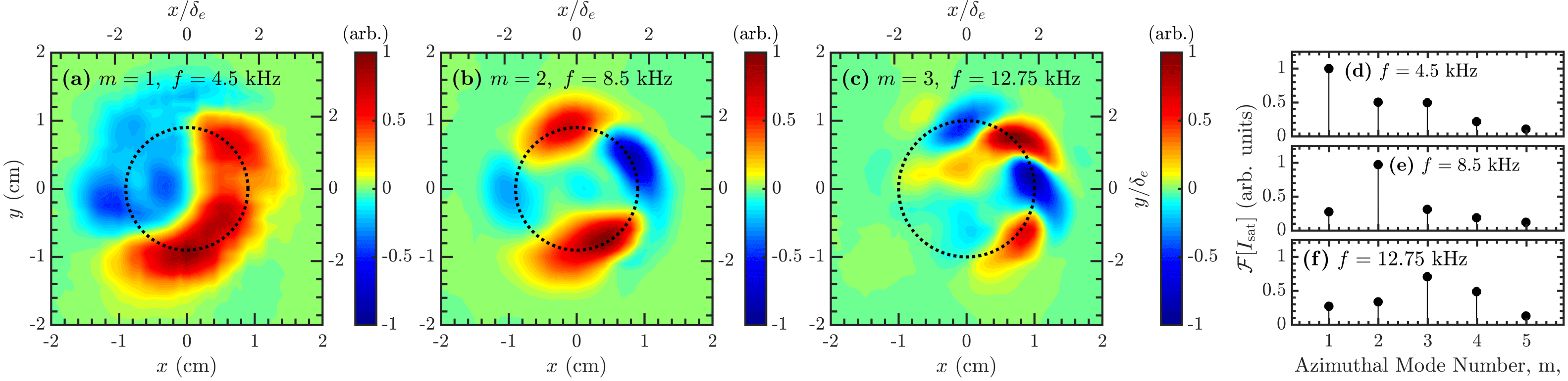
Figure 7. Mode structures for the three peaks observed in the power spectra on the outer gradient, indicated by dashed lines in the inset of figure 6(b). (a)
 $m=1$
mode at 4.5 kHz. (b)
$m=1$
mode at 4.5 kHz. (b)
 $m=2$
mode at 8.5 kHz. (c)
$m=2$
mode at 8.5 kHz. (c)
 $m=3$
mode at 12.75 kHz. The black dashed lines indicate the radius where the mode structures are peaked. The
$m=3$
mode at 12.75 kHz. The black dashed lines indicate the radius where the mode structures are peaked. The
 $x$
and
$x$
and
 $y$
scales have been shifted to centre the modes at (0, 0). (d–f) Azimuthal mode decomposition for each of (a–c), respectively.
$y$
scales have been shifted to centre the modes at (0, 0). (d–f) Azimuthal mode decomposition for each of (a–c), respectively.
There is a deviation from the exponentially decaying power spectrum below ∼20 kHz, shown in the inset of figure 6(b). Three distinct peaks occur in the power spectrum at 4.5 kHz, 8.5 kHz and 12.75 kHz. The mode structures for these frequencies can be obtained using cross-correlation techniques between signals from the moving and reference probe, shown in figure 7(a–c). This reveals that the modes have dominant azimuthal mode numbers of
 $m=1$
, 2 and 3, are peaked on the outer gradient of the filaments and have a striking azimuthal symmetry despite the asymmetric heating configuration. During the early stages of the plasma discharge (0–3 ms) these same global modes are present but with higher frequencies at approximately 7 kHz, 14 kHz and 20 kHz – indicating the
$m=1$
, 2 and 3, are peaked on the outer gradient of the filaments and have a striking azimuthal symmetry despite the asymmetric heating configuration. During the early stages of the plasma discharge (0–3 ms) these same global modes are present but with higher frequencies at approximately 7 kHz, 14 kHz and 20 kHz – indicating the
 $m=3$
mode from figure 4(d) maintains itself throughout the discharge while dropping in frequency. Towards the end of the discharge (12–15 ms) the same three modes are present and there is very little change in the frequencies from the middle of the discharge. Figure 7(d–f) shows the azimuthal mode decomposition using spatial Fourier analysis of figure 7(a–c), respectively, and confirms the visual conclusion of the dominant mode numbers at each frequency, but additionally shows there is significant power contained in other mode numbers; the observation of mixed mode numbers is similar to other drift wave experiments in cylindrical geometries and may indicate nonlinear coupling between the wave modes (Brandt et al.
Reference Brandt, Grulke, Klinger, Negrete, Bousselin, Brochard, Bonhomme and Oldenbürger2011; Thakur et al.
Reference Thakur, Brandt, Cui, Gosselin, Light and Tynan2014).
$m=3$
mode from figure 4(d) maintains itself throughout the discharge while dropping in frequency. Towards the end of the discharge (12–15 ms) the same three modes are present and there is very little change in the frequencies from the middle of the discharge. Figure 7(d–f) shows the azimuthal mode decomposition using spatial Fourier analysis of figure 7(a–c), respectively, and confirms the visual conclusion of the dominant mode numbers at each frequency, but additionally shows there is significant power contained in other mode numbers; the observation of mixed mode numbers is similar to other drift wave experiments in cylindrical geometries and may indicate nonlinear coupling between the wave modes (Brandt et al.
Reference Brandt, Grulke, Klinger, Negrete, Bousselin, Brochard, Bonhomme and Oldenbürger2011; Thakur et al.
Reference Thakur, Brandt, Cui, Gosselin, Light and Tynan2014).
To establish that there is no global mode present when the filaments are sufficiently separated a time trace from the gradient of one of the filaments from the far separation is shown in figure 6(d). The time trace shows the rapid development of a drift wave at 25 kHz (as shown on each filament in figure 4 b) that decreases in amplitude before the filament transitions to a more turbulent phase (Pace et al. Reference Pace, Shi, Maggs, Morales and Carter2008a ). The single shot spectrum displayed in figure 6(e) shows the highlighted 3 ms section of the time from figure 6(d). Clearly evident is the thermal wave (10 kHz), drift-Alfvén wave and harmonic sidebands from modulation of the drift-Alfvén waves by the thermal wave, and a baseline exponential frequency spectrum from Lorentzian shaped solitary pulses. This spectrum can be directly compared with previous work on single filaments (Burke et al. Reference Burke, Maggs and Morales2000a ,Reference Burke, Maggs and Morales b ; Pace et al. Reference Pace, Shi, Maggs, Morales and Carter2008a ) to conclude that the tri-filaments in the far separation are dominantly behaving as independent single filaments.
To better understand how the outer gradient is supporting these modes the temperature, density and pressure in figure 5 are interpolated to a polar grid with the origin selected to be the centre of the filament configuration. To investigate the azimuthal symmetry of the outer temperature gradient an average of 15° azimuthal averages through each filament is compared with an average of 15° azimuthal averages between each filament and the full azimuthal average of the configuration, shown in figure 8(a) for the
 $t=7.65~\text{ms}$
temperature profile (figure 5
e). As expected, the asymmetric heating configuration causes a flattop-like profile between the filaments and a profile peaked at ∼5 mm where the filaments are located. However, the gradient region beyond ∼7 mm shows more consistency between the full azimuthal average, the filaments and gaps between them. Figure 8(b) shows the full azimuthal averages of the pressure, temperature and density for the time
$t=7.65~\text{ms}$
temperature profile (figure 5
e). As expected, the asymmetric heating configuration causes a flattop-like profile between the filaments and a profile peaked at ∼5 mm where the filaments are located. However, the gradient region beyond ∼7 mm shows more consistency between the full azimuthal average, the filaments and gaps between them. Figure 8(b) shows the full azimuthal averages of the pressure, temperature and density for the time
 $t=1.65$
ms (figure 5
a–d) where the density is most varied; the values are normalized to the edge of the data collection plane. In both figures 8(a) and 8(b) the shaded region indicates the standard deviation in the azimuthal average. It is apparent that the gradient driving the modes is the temperature gradient and not the density gradient. The average temperature profile in figure 8(a) is accurately described by,
$t=1.65$
ms (figure 5
a–d) where the density is most varied; the values are normalized to the edge of the data collection plane. In both figures 8(a) and 8(b) the shaded region indicates the standard deviation in the azimuthal average. It is apparent that the gradient driving the modes is the temperature gradient and not the density gradient. The average temperature profile in figure 8(a) is accurately described by,
 $$\begin{eqnarray}T_{e}(r)=C_{1}+C_{2}\text{e}^{-C_{3}(r-C_{4})^{2}}+C_{5}(r+1.5~\text{cm})^{-4},\end{eqnarray}$$
where,
 $C_{1}=0.353~\text{eV}$
,
$C_{1}=0.353~\text{eV}$
,
 $C_{2}=1.957~\text{eV}$
,
$C_{2}=1.957~\text{eV}$
,
 $C_{3}=3.680~\text{cm}^{-2}$
,
$C_{3}=3.680~\text{cm}^{-2}$
,
 $C_{4}=0.469~\text{cm}$
,
$C_{4}=0.469~\text{cm}$
,
 $C_{5}=6.753~\text{eV}~\text{cm}^{4}$
.
$C_{5}=6.753~\text{eV}~\text{cm}^{4}$
.
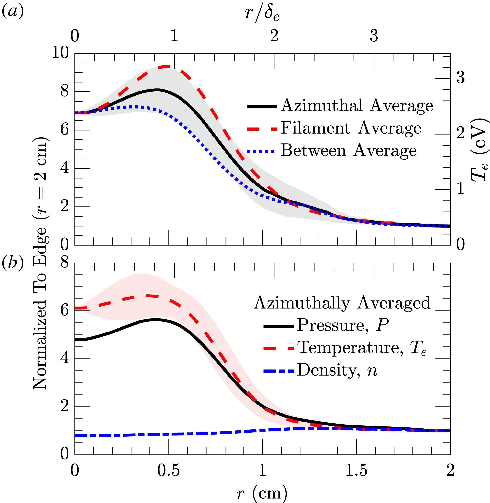
Figure 8. (a) Temperature profiles at
 $t=7.65~\text{ms}$
for radial cuts through the filaments (dashed red), between filaments (dotted blue), and the full azimuthal average (solid black). The standard deviation of the azimuthal average is given by the grey shaded region. (b) Azimuthal averages at
$t=7.65~\text{ms}$
for radial cuts through the filaments (dashed red), between filaments (dotted blue), and the full azimuthal average (solid black). The standard deviation of the azimuthal average is given by the grey shaded region. (b) Azimuthal averages at
 $t=1.65~\text{ms}$
of the pressure,
$t=1.65~\text{ms}$
of the pressure,
 $P$
(solid black), temperature,
$P$
(solid black), temperature,
 $T_{e}$
(dashed red), and density,
$T_{e}$
(dashed red), and density,
 $n$
(dash-dotted blue). The curves are normalized to their values at the edge of the three filament structure. The standard deviation in the temperature average is shown by the red shaded region, the pressure standard deviation is similar, while the standard deviation in density is comparatively negligible.
$n$
(dash-dotted blue). The curves are normalized to their values at the edge of the three filament structure. The standard deviation in the temperature average is shown by the red shaded region, the pressure standard deviation is similar, while the standard deviation in density is comparatively negligible.
4 Azimuthal flows and cathode model
The swept Langmuir probe measurements of the plasma potential allow a characterization of the transverse
 $\boldsymbol{E}\times \boldsymbol{B}$
flows generated by the well in the plasma potential at the centre of the filaments. Figure 9(a) shows the pressure at
$\boldsymbol{E}\times \boldsymbol{B}$
flows generated by the well in the plasma potential at the centre of the filaments. Figure 9(a) shows the pressure at
 $t=7.65~\text{ms}$
with the
$t=7.65~\text{ms}$
with the
 $\boldsymbol{E}\times \boldsymbol{B}$
flow arrows superimposed on top. The largest flows are concentrated on the outer gradient with some convective mixing in the centre region. Performing the same interpolation to a polar grid as was done for
$\boldsymbol{E}\times \boldsymbol{B}$
flow arrows superimposed on top. The largest flows are concentrated on the outer gradient with some convective mixing in the centre region. Performing the same interpolation to a polar grid as was done for
 $T_{e}$
,
$T_{e}$
,
 $n$
and
$n$
and
 $P$
the azimuthal average can be calculated, this is shown by the black circles in figure 9(b). The black dashed line shows an approximate fit to the data given by,
$P$
the azimuthal average can be calculated, this is shown by the black circles in figure 9(b). The black dashed line shows an approximate fit to the data given by,
 $$\begin{eqnarray}\unicode[STIX]{x1D719}(r)=C_{1}+C_{2}\text{e}^{-C_{3}(r-C_{4})^{2}}+C_{5}(r+3~\text{cm})^{-4},\end{eqnarray}$$
where
 $C_{1}=-3.309~\text{V}$
,
$C_{1}=-3.309~\text{V}$
,
 $C_{2}=-0.690~\text{V}$
,
$C_{2}=-0.690~\text{V}$
,
 $C_{3}=5.712~\text{cm}^{-2}$
,
$C_{3}=5.712~\text{cm}^{-2}$
,
 $C_{4}=0.397~\text{cm}$
,
$C_{4}=0.397~\text{cm}$
,
 $C_{5}=-75.410~\text{eV}~\text{cm}^{4}$
. The azimuthal average of the
$C_{5}=-75.410~\text{eV}~\text{cm}^{4}$
. The azimuthal average of the
 $\boldsymbol{E}\times \boldsymbol{B}$
flows,
$\boldsymbol{E}\times \boldsymbol{B}$
flows,
 $u_{\unicode[STIX]{x1D703}}$
, and a calculation from (4.1) are shown by the blue triangles and dashed blue line, respectively. The flow peaks at approximately
$u_{\unicode[STIX]{x1D703}}$
, and a calculation from (4.1) are shown by the blue triangles and dashed blue line, respectively. The flow peaks at approximately
 $2\times 10^{5}~\text{cm}~\text{s}^{-1}$
just outside the filament centres at
$2\times 10^{5}~\text{cm}~\text{s}^{-1}$
just outside the filament centres at
 ${\sim}7~\text{mm}$
and is nearly zero beyond
${\sim}7~\text{mm}$
and is nearly zero beyond
 ${\sim}1~\text{cm}$
. The flow shear is defined as,
${\sim}1~\text{cm}$
. The flow shear is defined as,
 $$\begin{eqnarray}\unicode[STIX]{x1D6FE}_{s}=r\frac{\unicode[STIX]{x2202}}{\unicode[STIX]{x2202}r}\left(\frac{u_{\unicode[STIX]{x1D703}}(r)}{r}\right).\end{eqnarray}$$
The azimuthal average of the flow shear is shown by the red squares in figure 9(b) and the calculation from (4.1) is shown by the dashed red line. The shear has opposite extrema on the inner (
 $3~\text{mm}$
) and outer (
$3~\text{mm}$
) and outer (
 $9~\text{mm}$
) gradients of the filaments with magnitudes of
$9~\text{mm}$
) gradients of the filaments with magnitudes of
 $5\times 10^{5}~\text{s}^{-1}$
.
$5\times 10^{5}~\text{s}^{-1}$
.
Figure 9. (a) Electron plasma beta plane at
 $t=7.65~\text{ms}$
with arrows indicating direction and magnitude of
$t=7.65~\text{ms}$
with arrows indicating direction and magnitude of
 $\boldsymbol{E}\times \boldsymbol{B}$
flows. (b) Azimuthal average of the radial structure of the plasma potential (left axis), azimuthal
$\boldsymbol{E}\times \boldsymbol{B}$
flows. (b) Azimuthal average of the radial structure of the plasma potential (left axis), azimuthal
 $\boldsymbol{E}\times \boldsymbol{B}$
flow velocity (right axis) and azimuthal flow shear (right axis). The error bars indicate the standard deviation of the azimuthal averaging.
$\boldsymbol{E}\times \boldsymbol{B}$
flow velocity (right axis) and azimuthal flow shear (right axis). The error bars indicate the standard deviation of the azimuthal averaging.
In a previous set of publications (Jin et al. Reference Jin, Poulos, Van Compernolle and Morales2019; Poulos Reference Poulos2019), a predictive analytical model for cathode operation in the LAPD afterglow was developed and tested. Here, an adaptation of that model is used to approximate the three-dimensional current system generated by the three-cathode arrangement.
The steady-current model expresses perpendicular and parallel currents in terms of a scalar plasma potential
 $\unicode[STIX]{x1D719}$
,
$\unicode[STIX]{x1D719}$
,
 $$\begin{eqnarray}\boldsymbol{j}_{\bot }=-\unicode[STIX]{x1D70E}_{\bot }\unicode[STIX]{x1D735}_{\bot }\unicode[STIX]{x1D719},\quad j_{\Vert }=-\unicode[STIX]{x1D70E}_{\Vert }\unicode[STIX]{x1D735}_{\Vert }\unicode[STIX]{x1D719},\end{eqnarray}$$
where for a partially ionized and strongly magnetized plasma, such as the afterglow of an LAPD discharge, the dominant contribution to the perpendicular conductivity is due to collisions between ions and neutrals
 $$\begin{eqnarray}\unicode[STIX]{x1D70E}_{\bot }=2.13\frac{e^{2}n\unicode[STIX]{x1D708}_{\text{in}}}{M\unicode[STIX]{x1D6FA}_{i}^{2}},\end{eqnarray}$$
and the parallel conductivity
 $\unicode[STIX]{x1D70E}_{\Vert }$
results from Coulomb collisions between electrons and ions
$\unicode[STIX]{x1D70E}_{\Vert }$
results from Coulomb collisions between electrons and ions
 $$\begin{eqnarray}\unicode[STIX]{x1D70E}_{\Vert }=1.96\frac{e^{2}n\unicode[STIX]{x1D70F}_{e}}{m},\end{eqnarray}$$
where,
 $m$
is the electron mass,
$m$
is the electron mass,
 $M$
is the ion mass,
$M$
is the ion mass,
 $e$
is the unit of electric charge,
$e$
is the unit of electric charge,
 $\unicode[STIX]{x1D6FA}_{i}=eB_{0}/Mc$
is the ion-cyclotron frequency and
$\unicode[STIX]{x1D6FA}_{i}=eB_{0}/Mc$
is the ion-cyclotron frequency and
 $\unicode[STIX]{x1D70F}_{e}$
is Braginskii’s electron collision time.
$\unicode[STIX]{x1D70F}_{e}$
is Braginskii’s electron collision time.
The nonlinear boundary condition at the interface between the plasma and cathode sheath ensures the total current in the cathode sheath matches the local current density in the plasma. See Poulos (Reference Poulos2019) for details.
A good approximation for the plasma potential formed by the three-cathode arrangement is obtained by superimposing three copies of the analytical solution for the single filament case (Poulos Reference Poulos2019, equation (14)). In general, if
 $\unicode[STIX]{x1D719}_{1}(r,z)$
is the azimuthally symmetric plasma potential for the single filament case, the plasma potential for multiple filaments located at
$\unicode[STIX]{x1D719}_{1}(r,z)$
is the azimuthally symmetric plasma potential for the single filament case, the plasma potential for multiple filaments located at
 $(x_{k},y_{k})$
, can be approximated as
$(x_{k},y_{k})$
, can be approximated as
 $$\begin{eqnarray}\unicode[STIX]{x1D719}_{\text{multi}}(x,y,z)=\mathop{\sum }_{k}\unicode[STIX]{x1D719}_{1}\left(\sqrt{(x-x_{k})^{2}+(y-y_{k})^{2}},z\right).\end{eqnarray}$$
Figure 10. (a) Prediction of plasma potential and
 $\boldsymbol{E}\times \boldsymbol{B}$
flows using the emissive cathode model. (b) The azimuthally averaged potential profile for the model prediction (red dashed) and experiment (solid black). The standard azimuthal standard deviation is indicated by shaded regions in red and grey for the model and experiment, respectively.
$\boldsymbol{E}\times \boldsymbol{B}$
flows using the emissive cathode model. (b) The azimuthally averaged potential profile for the model prediction (red dashed) and experiment (solid black). The standard azimuthal standard deviation is indicated by shaded regions in red and grey for the model and experiment, respectively.
The results of this model are presented in figure 10(a), which shows the predicted potential profile and
 $\boldsymbol{E}\times \boldsymbol{B}$
flows. A comparison of the azimuthal average of the predicted and measured potential profiles is shown in figure 10(a); the model accurately predicts the experimental profile, suggesting the observed transverse flows can be attributed to the emissive sheath boundary.
$\boldsymbol{E}\times \boldsymbol{B}$
flows. A comparison of the azimuthal average of the predicted and measured potential profiles is shown in figure 10(a); the model accurately predicts the experimental profile, suggesting the observed transverse flows can be attributed to the emissive sheath boundary.
5 Linear stability analysis
In this section, a stability analysis of the one-dimensional radial profiles is used to describe the quasi-axisymmetric modes observed on the outer gradient of the tri-filament structure. A derivation of the eigenvalue equation used here can be found in appendix A.
Assuming zeroth-order radial variation in density
 $n(r)$
, temperature
$n(r)$
, temperature
 $T_{e}(r)$
and azimuthal
$T_{e}(r)$
and azimuthal
 $E\times B$
velocity
$E\times B$
velocity
 $u_{\unicode[STIX]{x1D703}}(r)$
, the differential eigenvalue equation for the perturbed electric field
$u_{\unicode[STIX]{x1D703}}(r)$
, the differential eigenvalue equation for the perturbed electric field
 $E_{\Vert }^{\ast }$
takes the form
$E_{\Vert }^{\ast }$
takes the form
 $$\begin{eqnarray}\frac{1}{r}\frac{\unicode[STIX]{x2202}}{\unicode[STIX]{x2202}r}\left(r\frac{\tilde{\unicode[STIX]{x1D714}}+\text{i}\bar{\unicode[STIX]{x1D708}}_{\text{in}}}{\tilde{\unicode[STIX]{x1D714}}^{2}-\unicode[STIX]{x1D714}_{A}^{2}+\unicode[STIX]{x1D717}}\frac{\unicode[STIX]{x2202}E_{\Vert }^{\ast }}{\unicode[STIX]{x2202}r}\right)-\left[k_{\unicode[STIX]{x1D703}}^{2}\frac{\tilde{\unicode[STIX]{x1D714}}+\text{i}\bar{\unicode[STIX]{x1D708}}_{\text{in}}}{\tilde{\unicode[STIX]{x1D714}}^{2}-\unicode[STIX]{x1D714}_{A}^{2}+\unicode[STIX]{x1D717}}-k_{\unicode[STIX]{x1D703}}\frac{\unicode[STIX]{x2202}}{\unicode[STIX]{x2202}r}\left(\frac{\bar{\unicode[STIX]{x1D6FA}}_{R}}{\tilde{\unicode[STIX]{x1D714}}^{2}-\unicode[STIX]{x1D714}_{A}^{2}+\unicode[STIX]{x1D717}}\right)-\frac{\tilde{\unicode[STIX]{x1D714}}}{c^{2}}\unicode[STIX]{x1D716}_{\Vert }\right]E_{\Vert }^{\ast }=0.\end{eqnarray}$$
The rotation frequency shift, shear frequency and vorticity are respectively
 $$\begin{eqnarray}\unicode[STIX]{x1D6FA}_{R}=\frac{2u_{\unicode[STIX]{x1D703}}(r)}{r},\quad \unicode[STIX]{x1D6FE}_{s}=\frac{r}{2}\frac{\unicode[STIX]{x2202}\unicode[STIX]{x1D6FA}_{R}}{\unicode[STIX]{x2202}r},\quad {\mathcal{V}}=\unicode[STIX]{x1D6FA}_{R}+\unicode[STIX]{x1D6FE}_{s},\end{eqnarray}$$
and the Doppler-shifted frequency is
 $$\begin{eqnarray}\tilde{\unicode[STIX]{x1D714}}\equiv \unicode[STIX]{x1D714}-k_{\unicode[STIX]{x1D703}}u_{\unicode[STIX]{x1D703}}(r).\end{eqnarray}$$
The Alfvén frequency
 $\unicode[STIX]{x1D714}_{A}=k_{\Vert }v_{A}(r)=k_{\Vert }B_{0}/\sqrt{4\unicode[STIX]{x03C0}Mn(r)}$
carries an inverse square-root dependence on the plasma density. The response to rotation and ion–neutral collisions is characterized by the quantities
$\unicode[STIX]{x1D714}_{A}=k_{\Vert }v_{A}(r)=k_{\Vert }B_{0}/\sqrt{4\unicode[STIX]{x03C0}Mn(r)}$
carries an inverse square-root dependence on the plasma density. The response to rotation and ion–neutral collisions is characterized by the quantities
 $$\begin{eqnarray}\unicode[STIX]{x1D717}\equiv \frac{\unicode[STIX]{x1D708}_{\text{in}}^{2}+\unicode[STIX]{x1D6FA}_{R}^{2}}{1-\unicode[STIX]{x1D700}},\quad \bar{\unicode[STIX]{x1D708}}_{\text{in}}\equiv \frac{\unicode[STIX]{x1D708}_{\text{in}}}{1-\unicode[STIX]{x1D700}},\quad \bar{\unicode[STIX]{x1D6FA}}_{R}\equiv \frac{\unicode[STIX]{x1D6FA}_{R}}{1-\unicode[STIX]{x1D700}},\end{eqnarray}$$
where
 $$\begin{eqnarray}\unicode[STIX]{x1D700}\equiv \frac{(\tilde{\unicode[STIX]{x1D714}}+\text{i}\unicode[STIX]{x1D708}_{\text{in}})^{2}-\unicode[STIX]{x1D6FA}_{R}{\mathcal{V}}}{\unicode[STIX]{x1D714}_{A}^{2}},\end{eqnarray}$$
is related to the determinant of the ion-mobility tensor. The azimuthal and axial wavenumbers are
 $k_{\unicode[STIX]{x1D703}}=m/r$
and
$k_{\unicode[STIX]{x1D703}}=m/r$
and
 $k_{\Vert }=\unicode[STIX]{x03C0}/\tilde{L}$
, where
$k_{\Vert }=\unicode[STIX]{x03C0}/\tilde{L}$
, where
 $\tilde{L}$
is the effective length of the heated region. In this study, the effective length of the heated region is taken to be
$\tilde{L}$
is the effective length of the heated region. In this study, the effective length of the heated region is taken to be
 $8~\text{m}$
, a value that is inferred based on preliminary data and heat transport code results. In the limit
$8~\text{m}$
, a value that is inferred based on preliminary data and heat transport code results. In the limit
 $\unicode[STIX]{x1D708}_{\text{in}},\unicode[STIX]{x1D6FA}_{R}\rightarrow 0$
, equation (5.1) reproduces (17) of Peñano, Morales & Maggs (Reference Peñano, Morales and Maggs2000) with compressional coupling neglected.
$\unicode[STIX]{x1D708}_{\text{in}},\unicode[STIX]{x1D6FA}_{R}\rightarrow 0$
, equation (5.1) reproduces (17) of Peñano, Morales & Maggs (Reference Peñano, Morales and Maggs2000) with compressional coupling neglected.
The parallel dielectric
 $\unicode[STIX]{x1D716}_{\Vert }$
in (5.1) contains the kinetic response of the electrons and is given by
$\unicode[STIX]{x1D716}_{\Vert }$
in (5.1) contains the kinetic response of the electrons and is given by
 $$\begin{eqnarray}\unicode[STIX]{x1D716}_{\Vert }=1-\frac{\unicode[STIX]{x1D714}_{pi}^{2}}{\tilde{\unicode[STIX]{x1D714}}(\tilde{\unicode[STIX]{x1D714}}+\text{i}\unicode[STIX]{x1D708}_{\text{in}})}-\frac{k_{\text{De}}^{2}}{k_{\Vert }^{2}}\left(\frac{Z_{N}(\tilde{\unicode[STIX]{x1D701}}_{e})}{2}+\frac{\unicode[STIX]{x1D714}_{\ast }}{\tilde{\unicode[STIX]{x1D714}}}\right),\end{eqnarray}$$
where the generalized diamagnetic drift frequency
 $\unicode[STIX]{x1D714}_{\ast }$
takes the form
$\unicode[STIX]{x1D714}_{\ast }$
takes the form
 $$\begin{eqnarray}\unicode[STIX]{x1D714}_{\ast }=\frac{k_{\unicode[STIX]{x1D703}}c_{s}^{2}}{\unicode[STIX]{x1D6FA}_{i}}\left(\frac{Z_{N}(\tilde{\unicode[STIX]{x1D701}}_{e})}{2}\frac{\unicode[STIX]{x2202}\ln n}{\unicode[STIX]{x2202}r}+\frac{Z_{T}(\tilde{\unicode[STIX]{x1D701}}_{e})}{2}\frac{\unicode[STIX]{x2202}\ln T_{e}}{\unicode[STIX]{x2202}r}\right),\end{eqnarray}$$
and the argument
 $\tilde{\unicode[STIX]{x1D701}}_{e}=\tilde{\unicode[STIX]{x1D714}}/(\sqrt{2}k_{\Vert }\bar{v}_{e})$
is the Doppler-shifted phase velocity. Here
$\tilde{\unicode[STIX]{x1D701}}_{e}=\tilde{\unicode[STIX]{x1D714}}/(\sqrt{2}k_{\Vert }\bar{v}_{e})$
is the Doppler-shifted phase velocity. Here
 $\bar{v}_{e}=\sqrt{T_{e}/m}$
is the electron thermal velocity and
$\bar{v}_{e}=\sqrt{T_{e}/m}$
is the electron thermal velocity and
 $c_{s}=\sqrt{T_{e}/M}$
is the ion sound speed. In general, the functions
$c_{s}=\sqrt{T_{e}/M}$
is the ion sound speed. In general, the functions
 $Z_{N}$
and
$Z_{N}$
and
 $Z_{T}$
depend on the specific choice of collision operator used in (A 6). In the collisionless limit, the values of
$Z_{T}$
depend on the specific choice of collision operator used in (A 6). In the collisionless limit, the values of
 $Z_{N}$
and
$Z_{N}$
and
 $Z_{T}$
are related to derivatives of the usual plasma dispersion function
$Z_{T}$
are related to derivatives of the usual plasma dispersion function
 $Z(\unicode[STIX]{x1D701})$
by the expressions
$Z(\unicode[STIX]{x1D701})$
by the expressions
 $$\begin{eqnarray}Z_{N}(\unicode[STIX]{x1D701})=Z^{\prime }(\unicode[STIX]{x1D701}),\quad Z_{T}(\unicode[STIX]{x1D701})=-\frac{\unicode[STIX]{x1D701}}{2}Z^{\prime \prime }(\unicode[STIX]{x1D701}).\end{eqnarray}$$
Full kinetic collisionality can be incorporated with (10) in Peñano et al. (Reference Peñano, Morales and Maggs2000); however, problems associated with analyticity arise when considering the combined contributions of pitch-angle Coulomb scattering and sheared flow. Fair approximations for the collisional regime are obtained by taking the collisional limit of (10) in Peñano et al. (Reference Peñano, Morales and Maggs2000), which yields the expressions
 $$\begin{eqnarray}Z_{N}=-\text{i}2\frac{k_{\Vert }^{2}}{k_{D}^{2}}\frac{4\unicode[STIX]{x03C0}\unicode[STIX]{x1D70E}_{\Vert }}{\tilde{\unicode[STIX]{x1D714}}},\quad Z_{T}=-\text{i}5\frac{k_{\Vert }^{2}}{k_{D}^{2}}\frac{4\unicode[STIX]{x03C0}\unicode[STIX]{x1D70E}_{\Vert }}{\tilde{\unicode[STIX]{x1D714}}}.\end{eqnarray}$$
To aid in the comparison of model predictions with experiment, equation (A 6) is used to write the perturbed density in terms of the parallel electric field
 $$\begin{eqnarray}n_{1}=\frac{\text{i}k_{\text{De}}^{2}}{4\unicode[STIX]{x03C0}k_{\Vert }}\left(\frac{\unicode[STIX]{x1D714}_{\ast }}{\tilde{\unicode[STIX]{x1D714}}}+\frac{k_{\bot }c_{s}^{2}}{\unicode[STIX]{x1D6FA}_{i}\tilde{\unicode[STIX]{x1D714}}}\frac{\unicode[STIX]{x2202}\ln n_{0}}{\unicode[STIX]{x2202}r}+\frac{Z_{N}}{2}\right)E_{\Vert }^{\ast },\end{eqnarray}$$
which is used to compare the theoretical eigenfunctions with measured fluctuations in ion saturation current.
5.1 Numerical shooting method
Solutions to (5.1) are obtained with the numerical shooting method (Peñano, Morales & Maggs Reference Peñano, Morales and Maggs1997; Peñano et al.
Reference Peñano, Morales and Maggs2000; Poulos & Morales Reference Poulos and Morales2016). The method notes that gradients in zeroth-order quantities vanish in the regions
 $r\rightarrow 0$
and
$r\rightarrow 0$
and
 $r\rightarrow \infty$
, giving the asymptotic solutions of (5.1) precise analytic forms. In the limit of small
$r\rightarrow \infty$
, giving the asymptotic solutions of (5.1) precise analytic forms. In the limit of small
 $r$
, the solutions are Bessel functions of the first kind, while in the limit of large
$r$
, the solutions are Bessel functions of the first kind, while in the limit of large
 $r$
, the solutions are Hankel functions. For a given eigenvalue
$r$
, the solutions are Hankel functions. For a given eigenvalue
 $\unicode[STIX]{x1D714}$
, the two asymptotic solutions are integrated to a central mid-point via fourth-order Runge–Kutta numerical integration of (5.1). The complex value of
$\unicode[STIX]{x1D714}$
, the two asymptotic solutions are integrated to a central mid-point via fourth-order Runge–Kutta numerical integration of (5.1). The complex value of
 $\unicode[STIX]{x1D714}$
is then iterated until the difference of the two asymptotic solutions at the central mid-point vanishes within numerical tolerance. Convergence is typically obtained within 5–10 iterations.
$\unicode[STIX]{x1D714}$
is then iterated until the difference of the two asymptotic solutions at the central mid-point vanishes within numerical tolerance. Convergence is typically obtained within 5–10 iterations.
5.2 Results
The analysis is conducted using the experimentally observed one-dimensional azimuthal profiles of the temperature and potential, given in (3.1) and (4.1), respectively. Figure 11 shows predictions of the two-dimensional mode structures that are obtained from the parallel electric field for
 $m=1$
, 2 and 3, which can be compared with figure 7. A more detailed comparison is shown in figure 12(a–c) for each of modes
$m=1$
, 2 and 3, which can be compared with figure 7. A more detailed comparison is shown in figure 12(a–c) for each of modes
 $m=1$
, 2 and 3, respectively. The experimental temperature profile and (3.1) are shown in black, the experimental flow profile and (4.1) are shown in blue and the experimental and predicted mode profiles of ion saturation current are shown in red. For each of the observed modes, both the peak location and shape closely match the linear eigenmode analysis, however, there is some deviation possibly due to nonlinear effects discussed in the next section.
$m=1$
, 2 and 3, respectively. The experimental temperature profile and (3.1) are shown in black, the experimental flow profile and (4.1) are shown in blue and the experimental and predicted mode profiles of ion saturation current are shown in red. For each of the observed modes, both the peak location and shape closely match the linear eigenmode analysis, however, there is some deviation possibly due to nonlinear effects discussed in the next section.

Figure 11. Predicted two-dimensional mode structures for (a)
 $m=1$
, (b)
$m=1$
, (b)
 $m=2$
and (c)
$m=2$
and (c)
 $m=3$
. The perturbed density is displayed and black lines indicate where the mode structures are peaked radially.
$m=3$
. The perturbed density is displayed and black lines indicate where the mode structures are peaked radially.
Figure 12. Comparison of experimental radial mode structures with predictions of the collisional linear stability analysis (LSA). (a–c) Temperature in black (eV),
 $\boldsymbol{E}\times \boldsymbol{B}$
flow in blue (105 cm s-1) and radial mode structures in red (arbitrary units) for
$\boldsymbol{E}\times \boldsymbol{B}$
flow in blue (105 cm s-1) and radial mode structures in red (arbitrary units) for
 $m=1$
, 2 and 3 in (a), (b) and (c), respectively. The markers indicate the experimental observations and the solid lines represent inputs (temperature and flow) and output (mode structure) of the LSA. (d) The experimentally observed frequencies are indicated by the black squares, the predicted frequency in the collisionless regime by black circles, the predicted frequency in the collisional case by black triangles and the growth rates in the collisionless and collisional cases by red circles and triangles, respectively. To determine the predicted frequency
$m=1$
, 2 and 3 in (a), (b) and (c), respectively. The markers indicate the experimental observations and the solid lines represent inputs (temperature and flow) and output (mode structure) of the LSA. (d) The experimentally observed frequencies are indicated by the black squares, the predicted frequency in the collisionless regime by black circles, the predicted frequency in the collisional case by black triangles and the growth rates in the collisionless and collisional cases by red circles and triangles, respectively. To determine the predicted frequency
 $k_{z}L_{z}=\unicode[STIX]{x03C0}$
was used.
$k_{z}L_{z}=\unicode[STIX]{x03C0}$
was used.
Figure 12(d) compares the frequencies and growth rates predicted by the linear analysis with the observed frequencies in the experiment. The results demonstrate that there are severe limitations to the collisionless approximation. In the experiment, the observed frequency increases with azimuthal mode number, while the collisionless linear analysis predicts a decreasing frequency with increasing
 $m$
. Additionally, the
$m$
. Additionally, the
 $m=1$
eigenmode is predicted to have a negative growth rate where, clearly, the mode has a positive growth rate in the experiment. In contrast, the collisional approximation reproduces the observed trend in experimental frequencies and further yields positive growth rates for each of the modes. When the shear flow is neglected in the eigenmode solver the global eigenmode frequency is decreased by ∼20 % while the growth rate is increased by approximately ∼50 %. Artificially increasing the shear flow (the maxima in the azimuthal flow velocity) in the eigenmode solver produces a linearly decreasing growth rate until complete damping of the modes is obtained. However, the real part remains relatively constant (less than ∼30 % change).
$m=1$
eigenmode is predicted to have a negative growth rate where, clearly, the mode has a positive growth rate in the experiment. In contrast, the collisional approximation reproduces the observed trend in experimental frequencies and further yields positive growth rates for each of the modes. When the shear flow is neglected in the eigenmode solver the global eigenmode frequency is decreased by ∼20 % while the growth rate is increased by approximately ∼50 %. Artificially increasing the shear flow (the maxima in the azimuthal flow velocity) in the eigenmode solver produces a linearly decreasing growth rate until complete damping of the modes is obtained. However, the real part remains relatively constant (less than ∼30 % change).
Qualitatively, the complex radial eigenfunction in the regions with increased shear flow get phase shifted by a radially dependent complex phase, which physically corresponds to the eigenmode being dragged azimuthally in the direction of the imposed flow. The local stability is mainly determined by the imaginary parts of the
 $Z_{N}$
and
$Z_{N}$
and
 $Z_{T}$
functions. The global stability, however, is roughly determined by a summation of the local growth rates. As shear flow introduces a radially dependent Doppler shift in the
$Z_{T}$
functions. The global stability, however, is roughly determined by a summation of the local growth rates. As shear flow introduces a radially dependent Doppler shift in the
 $Z_{N}$
and
$Z_{N}$
and
 $Z_{T}$
functions, the sign of the local growth rate can reverse in radius. Therefore, the solutions to the resulting global eigenmode problem depend sensitively on the specific zeroth-order profiles. Accurate measurements of the experimental growth rates are not possible due to the fast-growing nature of the modes.
$Z_{T}$
functions, the sign of the local growth rate can reverse in radius. Therefore, the solutions to the resulting global eigenmode problem depend sensitively on the specific zeroth-order profiles. Accurate measurements of the experimental growth rates are not possible due to the fast-growing nature of the modes.
6 Discussion
In the tri-filament experiment the input power to the individual heat sources is nearly the same. However, when they are placed in close proximity the temperature distribution is not symmetric during the evolution, as illustrated in the two-dimensional temperature planes taken at different times and shown in figure 5(a,e,i). In the early phase non-azimuthally symmetric modes develop around the filaments and their interference leads to rapid mixing of the density, producing very uniform profiles (single filaments have non-uniform densities). These modes also rearrange the temperature such that the gradient is much reduced in the inner triangular region of the filaments and steepens in the outer triangular region. The drift-Alfvén modes that are excited in this outer region are more azimuthally symmetric and allow for a radial eigenmode analysis using azimuthally averaged profiles as input to the analytical model. The nature of these modes is similar to those found in the outer gradient of the single filament or in the filament from a hollow ring cathode.
There are several limitations to the linear stability analysis that are mentioned here. First, we have forgone a full kinetic description of electron–ion collisions, which are difficult to account for in the presence of shear flows; this will be the subject of future work. Based on previous studies of the linear stability of drift-Alfvén modes in the presence of thermal gradients and collisions without shear flows, the eigenmode stability is sensitive to finite electron–ion collisionality and form of the collision model (Peñano et al. Reference Peñano, Morales and Maggs2000).
Second, we used the flow velocity measured at one axial location near the cathode as input into the model. Due to efficient heat transport along the magnetic field the temperature has approximate axial homogeneity, whereas, the electric potential has stronger radial diffusion due to ion–neutral collisions which result in a radial electric field that falls off exponentially with distance from the cathode. To model an axially inhomogeneous potential profile a mean-field approach has been taken where the resulting axially averaged azimuthal flow is calculated using the plasma potential model which is estimated by reducing the measured azimuthal flow profiles at 2.5 m by approximately a factor of four. A two-dimensional radial–axial eigenmode analysis would be a necessary step to incorporate the simultaneous effects of axial and radial shear in the azimuthal flow.
A third possibility for the breakdown of linear theory is at early times, when the finite amplitude of the modes leads to nonlinear interaction. The fastest-growing modes may transfer energy into linearly stable modes through mode–mode coupling, leading to additional physics that is unaccounted for by the linear analysis.
There are two other notable features present in the probe data analysis of the experiment, shown in figure 6(c). The first is the presence of a cutoff feature in the power spectrum of the fluctuations which occurs at ∼70 kHz or
 $\unicode[STIX]{x1D714}/\unicode[STIX]{x1D6FA}_{i}\sim 0.2$
, and thus illustrates the Alfvénic nature of the modes (Morales et al.
Reference Morales, Maggs, Burke and Peñano1999). Similar exponential spectra in the density and magnetic field fluctuations with cutoff have been observed in various magnetized plasma configurations including the edge region of toroidal devices. The second feature is the rapid transition to a quasi-steady, broadband fluctuation spectrum as compared to the single filament case where several phases are observed; a quiescent phase, a time period dominated by large amplitude coherent modes and finally a transition to broadband turbulence.
$\unicode[STIX]{x1D714}/\unicode[STIX]{x1D6FA}_{i}\sim 0.2$
, and thus illustrates the Alfvénic nature of the modes (Morales et al.
Reference Morales, Maggs, Burke and Peñano1999). Similar exponential spectra in the density and magnetic field fluctuations with cutoff have been observed in various magnetized plasma configurations including the edge region of toroidal devices. The second feature is the rapid transition to a quasi-steady, broadband fluctuation spectrum as compared to the single filament case where several phases are observed; a quiescent phase, a time period dominated by large amplitude coherent modes and finally a transition to broadband turbulence.
7 Summary
In this study we have presented results from a basic heat transport experiment where three localized heat sources are embedded in a large, colder magnetized plasma. Each of the sources forms a field-aligned and elongated region of elevated electron temperature or temperature filament that is sufficiently far from the plasma boundaries. The cathode sources are mounted on probe drives for ease of variable separation and positioned in a triangular pattern. When the sources are separated by a distance greater than approximately two collisionless electron skin depths (
 ${\sim}2\unicode[STIX]{x1D6FF}_{e}$
, measured from edge to edge) they act as independent filaments, with growing drift-Alfvén modes on each of their respective gradients.
${\sim}2\unicode[STIX]{x1D6FF}_{e}$
, measured from edge to edge) they act as independent filaments, with growing drift-Alfvén modes on each of their respective gradients.
When the separation is reduced to approximately
 $\unicode[STIX]{x1D6FF}_{e}$
, the filaments interact strongly and the spatially overlapping drift-Alfvén modes on each filament induce enhanced particle and thermal transport, leading to a very flat density profile and flattened temperature profile in the inner triangular region of the filaments. The thermal gradient in the outer triangular region spontaneously generates a more azimuthally symmetric drift-Alfvén mode with a global radial extent of
$\unicode[STIX]{x1D6FF}_{e}$
, the filaments interact strongly and the spatially overlapping drift-Alfvén modes on each filament induce enhanced particle and thermal transport, leading to a very flat density profile and flattened temperature profile in the inner triangular region of the filaments. The thermal gradient in the outer triangular region spontaneously generates a more azimuthally symmetric drift-Alfvén mode with a global radial extent of
 ${\sim}2-3\unicode[STIX]{x1D6FF}_{e}$
.
${\sim}2-3\unicode[STIX]{x1D6FF}_{e}$
.
Along with the quasi-coherent drift-Alfvén modes there are azimuthal
 $\boldsymbol{E}\times \boldsymbol{B}$
shear flows that are induced by the emissive cathode. The electron source creates a negative potential well in the plasma that forms a radial electric field and corresponding azimuthal
$\boldsymbol{E}\times \boldsymbol{B}$
shear flows that are induced by the emissive cathode. The electron source creates a negative potential well in the plasma that forms a radial electric field and corresponding azimuthal
 $\boldsymbol{E}\times \boldsymbol{B}$
flow. The extension of an emissive cathode model (Poulos Reference Poulos2019) predicts the plasma potential for the triple cathode set-up and agrees with the experiment. The fitted potential profiles give the azimuthal
$\boldsymbol{E}\times \boldsymbol{B}$
flow. The extension of an emissive cathode model (Poulos Reference Poulos2019) predicts the plasma potential for the triple cathode set-up and agrees with the experiment. The fitted potential profiles give the azimuthal
 $\boldsymbol{E}\times \boldsymbol{B}$
flow profile that is input into the eigenmode solver.
$\boldsymbol{E}\times \boldsymbol{B}$
flow profile that is input into the eigenmode solver.
A linear kinetic theory for drift-Alfvén modes that includes shear flows, ion–neutral and ion–electron collisions and uses fits to the azimuthally averaged density, temperature and
 $\boldsymbol{E}\times \boldsymbol{B}$
flows matches well with the observed mode structures. Nonlinear gyrokinetic modelling is currently being carried out to establish the time scales of nonlinear mode–mode interactions which could also account for the deviation from linear theory.
$\boldsymbol{E}\times \boldsymbol{B}$
flows matches well with the observed mode structures. Nonlinear gyrokinetic modelling is currently being carried out to establish the time scales of nonlinear mode–mode interactions which could also account for the deviation from linear theory.
Acknowledgements
Authors S.K. and R.D.S. acknowledge support from the Natural Sciences and Engineering Research Council of Canada (NSERC), the experiments were performed at the Basic Plasma Science Facility supported by DOE and NSF, with major facility instrumentation developed via an NSF award AGS-9724366.
Appendix A. Derivation of eigenvalue equation
For the analysis considered here, the quantity
 $u_{\bot }$
is the
$u_{\bot }$
is the
 $\boldsymbol{E}\times \boldsymbol{B}$
velocity perpendicular to the zeroth-order magnetic field and
$\boldsymbol{E}\times \boldsymbol{B}$
velocity perpendicular to the zeroth-order magnetic field and
 $\text{d}/\text{d}t$
is the corresponding convective derivative,
$\text{d}/\text{d}t$
is the corresponding convective derivative,
 $$\begin{eqnarray}\boldsymbol{u}_{\bot }\equiv \frac{c}{B_{\Vert }}\boldsymbol{E}_{\bot }\times \hat{z},\quad \frac{\text{d}}{\text{d}t}\equiv \frac{\unicode[STIX]{x2202}}{\unicode[STIX]{x2202}t}+\boldsymbol{u}_{\bot }\boldsymbol{\cdot }\unicode[STIX]{x1D735}_{\bot }.\end{eqnarray}$$
The quantity
 $E_{\Vert }^{\ast }$
denotes the parallel electric field in the frame moving with the perpendicular velocity and
$E_{\Vert }^{\ast }$
denotes the parallel electric field in the frame moving with the perpendicular velocity and
 $\unicode[STIX]{x1D735}_{\Vert }^{\ast }$
is the component of the derivative pointing along the magnetic field
$\unicode[STIX]{x1D735}_{\Vert }^{\ast }$
is the component of the derivative pointing along the magnetic field
 $$\begin{eqnarray}E_{\Vert }^{\ast }\equiv \frac{\boldsymbol{B}\boldsymbol{\cdot }\boldsymbol{E}}{B_{\Vert }},\quad \unicode[STIX]{x1D735}_{\Vert }^{\ast }\equiv \frac{\boldsymbol{B}\boldsymbol{\cdot }\unicode[STIX]{x1D735}}{B_{\Vert }}.\end{eqnarray}$$
With these definitions,
 $E_{\bot }$
is eliminated from the parallel and perpendicular components of Faraday’s law, yielding
$E_{\bot }$
is eliminated from the parallel and perpendicular components of Faraday’s law, yielding
 $$\begin{eqnarray}\frac{\text{d}B_{\Vert }}{\text{d}t}+B_{\Vert }\unicode[STIX]{x1D735}_{\bot }\boldsymbol{\cdot }\boldsymbol{u}_{\bot }=0,\end{eqnarray}$$
and
 $$\begin{eqnarray}\frac{\text{d}}{\text{d}t}\left(\frac{\boldsymbol{B}_{\bot }}{B_{\Vert }}\right)=\unicode[STIX]{x1D735}_{\Vert }^{\ast }\boldsymbol{u}_{\bot }+\frac{c}{B_{\Vert }}\hat{z}\times \unicode[STIX]{x1D735}_{\bot }E_{\Vert }^{\ast }.\end{eqnarray}$$
Assuming cold ions, quasi-neutrality and time scales longer than the ion-cyclotron period, the equation of ion motion and Ampere’s law are combined to yield
 $$\begin{eqnarray}Mn\left(\frac{\text{d}}{\text{d}t}+u_{\Vert }\unicode[STIX]{x1D735}_{\Vert }^{\ast }+\unicode[STIX]{x1D708}_{\text{in}}\right)\boldsymbol{u}=\frac{B_{\Vert }\unicode[STIX]{x1D735}_{\Vert }^{\ast }\boldsymbol{B}_{\bot }}{4\unicode[STIX]{x03C0}}-\unicode[STIX]{x1D735}p,\end{eqnarray}$$
where
 $u_{\Vert }$
is the parallel velocity of the ions and
$u_{\Vert }$
is the parallel velocity of the ions and
 $p=B^{2}/8\unicode[STIX]{x03C0}+nT_{e}$
.
$p=B^{2}/8\unicode[STIX]{x03C0}+nT_{e}$
.
The response of the electrons is determined from a drift-kinetic description
 $$\begin{eqnarray}\left(\frac{\text{d}}{\text{d}t}+v_{\Vert }\unicode[STIX]{x1D735}_{\Vert }^{\ast }-\frac{e}{m}E_{\Vert }^{\ast }\frac{\unicode[STIX]{x2202}}{\unicode[STIX]{x2202}v_{\Vert }}\right)\frac{f_{e}}{B_{\Vert }}=\frac{{\mathcal{C}}[f_{e}]}{B_{\Vert }},\end{eqnarray}$$
where
 ${\mathcal{C}}[f_{e}]$
is the electron collision operator. The system of equations is closed with the parallel component of Ampère’s law
${\mathcal{C}}[f_{e}]$
is the electron collision operator. The system of equations is closed with the parallel component of Ampère’s law
 $$\begin{eqnarray}\unicode[STIX]{x1D735}_{\bot }\boldsymbol{\cdot }(\boldsymbol{B}_{\bot }\times \hat{z})=\frac{4\unicode[STIX]{x03C0}}{c}e\left(nu_{\Vert }-\int \text{d}v_{\Vert }\;v_{\Vert }f_{e}\right).\end{eqnarray}$$
Neglecting
 $B_{\Vert }$
fluctuations, equation (A 5) is perturbed and transformed, giving
$B_{\Vert }$
fluctuations, equation (A 5) is perturbed and transformed, giving
 $$\begin{eqnarray}(\tilde{\unicode[STIX]{x1D714}}+\text{i}\unicode[STIX]{x1D708}_{\text{in}}+\text{i}{\mathcal{V}}\hat{\unicode[STIX]{x1D703}}\hat{r}-\text{i}\unicode[STIX]{x1D6FA}_{R}\hat{r}\hat{\unicode[STIX]{x1D703}})\boldsymbol{u}_{\bot }=-\frac{k_{\Vert }^{2}v_{A}^{2}}{k_{\Vert }B_{\Vert }}\boldsymbol{B}_{\bot },\end{eqnarray}$$
which is inverted to give
 $u_{\bot }$
in terms of
$u_{\bot }$
in terms of
 $B_{\bot }$
,
$B_{\bot }$
,
 $$\begin{eqnarray}\boldsymbol{u}_{\bot }=\frac{-1}{k_{\Vert }B_{\Vert }\unicode[STIX]{x1D700}}(\tilde{\unicode[STIX]{x1D714}}+\text{i}\unicode[STIX]{x1D708}_{\text{in}}-\text{i}{\mathcal{V}}\hat{\unicode[STIX]{x1D703}}\hat{r}+\text{i}\unicode[STIX]{x1D6FA}_{R}\hat{r}\hat{\unicode[STIX]{x1D703}})\boldsymbol{B}_{\bot },\end{eqnarray}$$
where
 $$\begin{eqnarray}\unicode[STIX]{x1D700}=\frac{(\tilde{\unicode[STIX]{x1D714}}+\text{i}\unicode[STIX]{x1D708}_{\text{in}})^{2}-\unicode[STIX]{x1D6FA}_{R}{\mathcal{V}}}{\unicode[STIX]{x1D714}_{A}^{2}}.\end{eqnarray}$$
Perturbing and transforming (A 4)
 $$\begin{eqnarray}(\tilde{\unicode[STIX]{x1D714}}-\text{i}\unicode[STIX]{x1D6FE}_{s}\hat{\unicode[STIX]{x1D703}}\hat{r})\boldsymbol{B}_{\bot }=-k_{\Vert }B_{\Vert }\boldsymbol{u}_{\bot }+\text{i}c\hat{z}\times \unicode[STIX]{x1D735}_{\bot }E_{\Vert }^{\ast },\end{eqnarray}$$
and eliminating
 $u_{\bot }$
, gives
$u_{\bot }$
, gives
 $$\begin{eqnarray}[\unicode[STIX]{x1D700}(\tilde{\unicode[STIX]{x1D714}}+\text{i}\unicode[STIX]{x1D6FE}_{s}\hat{r}\hat{\unicode[STIX]{x1D703}})-(\tilde{\unicode[STIX]{x1D714}}+\text{i}\unicode[STIX]{x1D708}_{\text{in}}-\text{i}\unicode[STIX]{x1D6FA}_{R}\hat{\unicode[STIX]{x1D703}}\hat{r}+\text{i}{\mathcal{V}}\hat{r}\hat{\unicode[STIX]{x1D703}})]\boldsymbol{B}_{\bot }\times \hat{z}=\text{i}\unicode[STIX]{x1D700}c\unicode[STIX]{x1D735}_{\bot }E_{\Vert }^{\ast }.\end{eqnarray}$$
Solving for
 $B_{\bot }\times \hat{z}$
in terms of
$B_{\bot }\times \hat{z}$
in terms of
 $E_{\Vert }^{\ast }$
yields
$E_{\Vert }^{\ast }$
yields
 $$\begin{eqnarray}\displaystyle \boldsymbol{B}_{\bot }\times \hat{z} & = & \displaystyle \frac{\text{i}c}{(1-\unicode[STIX]{x1D700})(\unicode[STIX]{x1D714}_{A}^{2}-\tilde{\unicode[STIX]{x1D714}}^{2})-\unicode[STIX]{x1D708}_{\text{in}}^{2}-\unicode[STIX]{x1D6FA}_{R}^{2}}\nonumber\\ \displaystyle & & \displaystyle \times \,[\unicode[STIX]{x1D700}(\tilde{\unicode[STIX]{x1D714}}-\text{i}\unicode[STIX]{x1D6FE}_{s}\hat{r}\hat{\unicode[STIX]{x1D703}})-(\tilde{\unicode[STIX]{x1D714}}+\text{i}\unicode[STIX]{x1D708}_{\text{in}}+\text{i}\unicode[STIX]{x1D6FA}_{R}\hat{\unicode[STIX]{x1D703}}\hat{r}-\text{i}{\mathcal{V}}\hat{r}\hat{\unicode[STIX]{x1D703}})]\boldsymbol{\cdot }\unicode[STIX]{x1D735}_{\bot }E_{\Vert }^{\ast }.\end{eqnarray}$$
Defining the quantities
 $$\begin{eqnarray}\unicode[STIX]{x1D717}\equiv \frac{\unicode[STIX]{x1D708}_{\text{in}}^{2}+\unicode[STIX]{x1D6FA}_{R}^{2}}{1-\unicode[STIX]{x1D700}},\quad \bar{\unicode[STIX]{x1D708}}_{\text{in}}=\frac{\unicode[STIX]{x1D708}_{\text{in}}}{1-\unicode[STIX]{x1D700}},\quad \bar{\unicode[STIX]{x1D6FA}}_{R}=\frac{\bar{\unicode[STIX]{x1D6FA}}_{R}}{1-\unicode[STIX]{x1D700}},\end{eqnarray}$$
the radial and azimuthal components of
 $\boldsymbol{B}_{\bot }\times \hat{z}$
are explicitly
$\boldsymbol{B}_{\bot }\times \hat{z}$
are explicitly
 $$\begin{eqnarray}(\boldsymbol{B}_{\bot }\times \hat{z})_{r}=\frac{-\text{i}c}{\unicode[STIX]{x1D714}_{A}^{2}-\tilde{\unicode[STIX]{x1D714}}^{2}-\unicode[STIX]{x1D717}}\left[(\tilde{\unicode[STIX]{x1D714}}+\text{i}\bar{\unicode[STIX]{x1D708}}_{\text{in}})\frac{\unicode[STIX]{x2202}}{\unicode[STIX]{x2202}r}+k_{\unicode[STIX]{x1D703}}\bar{\unicode[STIX]{x1D6FA}}_{R}\right]E_{\Vert }^{\ast },\end{eqnarray}$$
and
 $$\begin{eqnarray}(\boldsymbol{B}_{\bot }\times \hat{z})_{\unicode[STIX]{x1D703}}=\frac{-\text{i}c}{\unicode[STIX]{x1D714}_{A}^{2}-\tilde{\unicode[STIX]{x1D714}}^{2}-\unicode[STIX]{x1D717}}\left[(\tilde{\unicode[STIX]{x1D714}}+\text{i}\bar{\unicode[STIX]{x1D708}}_{\text{in}})\text{i}k_{\unicode[STIX]{x1D703}}+\text{i}\bar{\unicode[STIX]{x1D6FA}}_{R}\frac{\unicode[STIX]{x2202}}{\unicode[STIX]{x2202}r}\right]E_{\Vert }^{\ast }.\end{eqnarray}$$
Inserting these expressions into Ampère’s law gives
 $$\begin{eqnarray}\frac{1}{r}\frac{\unicode[STIX]{x2202}}{\unicode[STIX]{x2202}r}\left(r\frac{\tilde{\unicode[STIX]{x1D714}}+\text{i}\bar{\unicode[STIX]{x1D708}}_{\text{in}}}{\tilde{\unicode[STIX]{x1D714}}^{2}-\unicode[STIX]{x1D714}_{A}^{2}+\unicode[STIX]{x1D717}}\frac{\unicode[STIX]{x2202}E_{\Vert }^{\ast }}{\unicode[STIX]{x2202}r}\right)-\left[k_{\unicode[STIX]{x1D703}}^{2}\frac{\tilde{\unicode[STIX]{x1D714}}+\text{i}\bar{\unicode[STIX]{x1D708}}_{\text{in}}}{\tilde{\unicode[STIX]{x1D714}}^{2}-\unicode[STIX]{x1D714}_{A}^{2}+\unicode[STIX]{x1D717}}-k_{\unicode[STIX]{x1D703}}\frac{\unicode[STIX]{x2202}}{\unicode[STIX]{x2202}r}\left(\frac{\bar{\unicode[STIX]{x1D6FA}}_{R}}{\tilde{\unicode[STIX]{x1D714}}^{2}-\unicode[STIX]{x1D714}_{A}^{2}+\unicode[STIX]{x1D717}}\right)\right]E_{\Vert }^{\ast }=\frac{4\unicode[STIX]{x03C0}}{\text{i}c^{2}}j_{\Vert }.\end{eqnarray}$$
The parallel current density
 $j_{\Vert }$
is essentially identical to (8) in Peñano et al. (Reference Peñano, Morales and Maggs2000), except that the frequencies are Doppler shifted and ion–neutral collisions are added to the parallel response
$j_{\Vert }$
is essentially identical to (8) in Peñano et al. (Reference Peñano, Morales and Maggs2000), except that the frequencies are Doppler shifted and ion–neutral collisions are added to the parallel response
 $$\begin{eqnarray}j_{\Vert }=\frac{\text{i}\tilde{\unicode[STIX]{x1D714}}}{4\unicode[STIX]{x03C0}}\left[\frac{\unicode[STIX]{x1D714}_{pi}^{2}}{\tilde{\unicode[STIX]{x1D714}}(\tilde{\unicode[STIX]{x1D714}}+\text{i}\unicode[STIX]{x1D708}_{\text{in}})}+\frac{k_{D}^{2}}{k_{\Vert }^{2}}\left(Z_{N}(\tilde{\unicode[STIX]{x1D701}},\bar{\unicode[STIX]{x1D708}})+2\frac{\unicode[STIX]{x1D714}_{\ast }}{\tilde{\unicode[STIX]{x1D714}}}\right)\right]E_{\Vert }^{\ast }.\end{eqnarray}$$


