


1 Introduction
Let
 $G=\mathrm {GL}(2,\mathbb {C}), \mathrm {SL}(2,\mathbb {C})$
. We denote by
$G=\mathrm {GL}(2,\mathbb {C}), \mathrm {SL}(2,\mathbb {C})$
. We denote by
 $\mathcal {M}_{Dol}^G$
be the moduli space of G-Higgs bundles of rank 2 and degree 0 on genus 2 curve C. In this article we want to study the cohomological properties of this space from a Hodge-theoretic point of view. The main problem in doing that is that the moduli space is singular and many fundamental theorems like Poincaré duality or Hard-Lefschetz theorem fail for ordinary cohomology groups. To overcome this fact one might opt for two solutions: to resolve singularities or to consider a different cohomological invariant, namely, intersection cohomology. Here we adopt both strategies, showing how they are strongly interrelated. We first show the following result.
$\mathcal {M}_{Dol}^G$
be the moduli space of G-Higgs bundles of rank 2 and degree 0 on genus 2 curve C. In this article we want to study the cohomological properties of this space from a Hodge-theoretic point of view. The main problem in doing that is that the moduli space is singular and many fundamental theorems like Poincaré duality or Hard-Lefschetz theorem fail for ordinary cohomology groups. To overcome this fact one might opt for two solutions: to resolve singularities or to consider a different cohomological invariant, namely, intersection cohomology. Here we adopt both strategies, showing how they are strongly interrelated. We first show the following result.
Theorem 1.1. Let C be a curve of genus 2 and let
 $\mathcal {M}_{Dol}^G$
be the moduli space of G-Higgs bundles of rank 2 and degree 0 on C. Then there exists a symplectic desingularisation
$\mathcal {M}_{Dol}^G$
be the moduli space of G-Higgs bundles of rank 2 and degree 0 on C. Then there exists a symplectic desingularisation
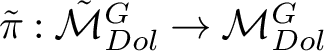 $\tilde {\pi }:\tilde {\mathcal {M}}_{Dol}^G\rightarrow \mathcal {M}_{Dol}^G$
.
$\tilde {\pi }:\tilde {\mathcal {M}}_{Dol}^G\rightarrow \mathcal {M}_{Dol}^G$
.
This theorem was obtained independently by Bellamy and Schedler in [Reference Bellamy and Schedler3] in the language of character varieties. In fact, it is well known that, by the nonabelian Hodge theorem [Reference Simpson39],
 $\mathcal {M}_{Dol}^G$
is real analytic isomorphic to the character variety of representations of the fundamental group of C into G. The equivalence with our result is obtained by applying the isosingularity principle [Reference Simpson39, Theorem 10.6], which states that two corresponding singular points on the moduli spaces admit isomorphic étale neighbourhoods. Having a symplectic desingularisation is indeed a special feature of this moduli space: in fact, apart from rank 2 and degree 0 G-Higgs bundles on a genus 2 curve, the only other case in which a symplectic resolution exists is that of degree 0 G-Higgs bundles of arbitrary rank on an elliptic curve. For higher genera and ranks, the moduli spaces do not admit a symplectic desingularisation; see [Reference Tirelli40] and [Reference Kiem and Yoo24].
$\mathcal {M}_{Dol}^G$
is real analytic isomorphic to the character variety of representations of the fundamental group of C into G. The equivalence with our result is obtained by applying the isosingularity principle [Reference Simpson39, Theorem 10.6], which states that two corresponding singular points on the moduli spaces admit isomorphic étale neighbourhoods. Having a symplectic desingularisation is indeed a special feature of this moduli space: in fact, apart from rank 2 and degree 0 G-Higgs bundles on a genus 2 curve, the only other case in which a symplectic resolution exists is that of degree 0 G-Higgs bundles of arbitrary rank on an elliptic curve. For higher genera and ranks, the moduli spaces do not admit a symplectic desingularisation; see [Reference Tirelli40] and [Reference Kiem and Yoo24].
By a theorem of Kaledin (see [Reference Kaledin23]) all symplectic resolutions are semismall (cf. Section 1) and such a property allows application of a special version of the decomposition theorem of Beilinson, Bernstein and Deligne [Reference Beilinson, Bernstein and Deligne2] that asserts that the cohomology of the resolution
 $\tilde {\mathcal {M}}_{Dol}^G$
splits as a direct sum of the intersection cohomology of
$\tilde {\mathcal {M}}_{Dol}^G$
splits as a direct sum of the intersection cohomology of
 $\mathcal {M}_{Dol}^G$
with some summands supported on the singular locus, which we are able to determine. Given this theorem, if we compute the ordinary cohomology of the resolution and subtract the contributions coming from the summands on the singular locus, we end up with the intersection cohomology of
$\mathcal {M}_{Dol}^G$
with some summands supported on the singular locus, which we are able to determine. Given this theorem, if we compute the ordinary cohomology of the resolution and subtract the contributions coming from the summands on the singular locus, we end up with the intersection cohomology of
 $\mathcal {M}_{Dol}^G$
. More precisely, we prove the following result.
$\mathcal {M}_{Dol}^G$
. More precisely, we prove the following result.
Theorem 1.2. Let C be a smooth projective complex curve of genus 2 and let
 $\mathcal {M}_{Dol}^{\mathrm {G}}$
be the moduli space of G-Higgs bundles on C for
$\mathcal {M}_{Dol}^{\mathrm {G}}$
be the moduli space of G-Higgs bundles on C for
 $G=\mathrm {GL}(2,\mathbb {C}), \mathrm {SL}(2,\mathbb {C})$
. Then the intersection Poincaré polynomials of
$G=\mathrm {GL}(2,\mathbb {C}), \mathrm {SL}(2,\mathbb {C})$
. Then the intersection Poincaré polynomials of
 $\mathcal {M}_{Dol}^G$
are
$\mathcal {M}_{Dol}^G$
are
 $$ \begin{align*} IP_t(\mathcal{M}_{Dol}^{\mathrm{SL}}) &=1+t^2+17t^4+17t^6;\\ IP_t(\mathcal{M}_{Dol}^{\mathrm{GL}}) &= 1+4t+7t^2+8t^3+9t^4+12t^5+15t^6+16t^7+14t^8+8t^9+2t^{10}. \end{align*} $$
Moreover, the Hodge structure on the intersection cohomology of
 $\mathcal {M}_{Dol}^G$
is pure and the Hodge diamond is
$\mathcal {M}_{Dol}^G$
is pure and the Hodge diamond is
 $$ \begin{align*} G=\mathrm{SL}(2,\mathbb{C}): \begin{array}{l|ccc} {\it 0}&{\it (0,0)}&\\ &&\\ {\it 2}&{\it (1,1)}&\\ &&\\ {\it 4}&{\it 17(2,2)}&\\ &&\\ {\it 6}&{\it 17(3,3)}&\\ \end{array} \end{align*} $$
 $$ \begin{align*} G=\mathrm{GL}(2,\mathbb{C}): \begin{array}{l|ccc} {\it 0}&&{\it (0,0)}&\\ {\it 1}&{\it 2(1,0)}&&{\it 2(0,1)}\\ {\it 2}&{\it (2,0)}&{\it 5(1,1)}&{\it (0,2)}\\ {\it 3}&{\it 4(2,1)}&&{\it 4(1,2)}\\ {\it 4}&{\it (1,3)}&{\it 7(2,2)}&{\it (3,1)}\\ {\it 5}&{\it 6(3,2)}&&{\it 6(2,3)}\\ {\it 6}&{\it 2(4,2)}&{\it 11(3,3)}&{\it 2(2,4)}\\ {\it 7}&{\it 8(4,3)}&&{\it 8(3,4)}\\ {\it 8}&{\it 2(5,3)}&{\it 10(2,2)}&{\it 2(3,5)}\\ {\it 9}&{\it 4(5,4)}&&{\it 4(4,5)}\\ {\it 10}&&{\it 2(5,5)}&.\\ \end{array} \end{align*} $$
Let us now give a sketch of the proof of these two results. The resolution is constructed using a strategy developed by O’Grady in [Reference O’Grady34] and [Reference O’Grady35] to desingularise moduli spaces of sheaves on K3 or abelian surfaces. With this procedure, O’Grady obtains two new examples of compact hyperkähler manifolds up to birational equivalence, which are usually denoted by OG10 and OG6. Such examples have dimension, respectively 10 and 6, as
 $\mathcal {M}_{Dol}^{\mathrm {GL}}$
and
$\mathcal {M}_{Dol}^{\mathrm {GL}}$
and
 $\mathcal {M}_{Dol}^{\mathrm {SL}}$
. Indeed, more is true: applying methods similar to those in [Reference De Cataldo, Maulik and Shen6] and [Reference Donagi, Ein and Lazarsfeld13], one can show that there exists a degeneration of hyperkähler manifolds from O’Grady moduli spaces to those of Higgs bundles. In view of this, the singularities of
$\mathcal {M}_{Dol}^{\mathrm {SL}}$
. Indeed, more is true: applying methods similar to those in [Reference De Cataldo, Maulik and Shen6] and [Reference Donagi, Ein and Lazarsfeld13], one can show that there exists a degeneration of hyperkähler manifolds from O’Grady moduli spaces to those of Higgs bundles. In view of this, the singularities of
 $\mathcal {M}_{Dol}^G$
have isomorphic local description to those of O’Grady examples, as we show in Section 3.
$\mathcal {M}_{Dol}^G$
have isomorphic local description to those of O’Grady examples, as we show in Section 3.
The singular locus
 $\Sigma ^G$
is given by Higgs bundles, which can be written as a direct sum of two Higgs line bundles. For example, for
$\Sigma ^G$
is given by Higgs bundles, which can be written as a direct sum of two Higgs line bundles. For example, for
 $G=\mathrm {GL}(2,\mathbb {C})$
the singular locus stratifies as
$G=\mathrm {GL}(2,\mathbb {C})$
the singular locus stratifies as
 $$ \begin{align*} \Sigma^G &=\left\lbrace (L,\phi)\oplus (M,\psi)\mid L,M\in Jac(C), \text{ and } \phi,\psi\in H^0(K_C) \right \rbrace;\\ \Omega^G &=\left\lbrace (L,\phi)\oplus (L,\phi)\mid L\in Jac(C), \text{ and } \phi\in H^0(K_C) \right \rbrace. \end{align*} $$
It is easy to see that in this case
 $\Sigma ^G$
is isomorphic to the symmetric product
$\Sigma ^G$
is isomorphic to the symmetric product
 $Sym^2(Jac(C)\times H^0(K_C))$
; thus, it is a singular eightfold with finite quotient singularities along
$Sym^2(Jac(C)\times H^0(K_C))$
; thus, it is a singular eightfold with finite quotient singularities along
 $\Omega ^G$
. The description for
$\Omega ^G$
. The description for
 $G=\mathrm {SL}(2,\mathbb {C})$
is analogous mutatis mutandis.
$G=\mathrm {SL}(2,\mathbb {C})$
is analogous mutatis mutandis.
In both cases, the resolution is obtained by a single blow up along the locus
 $\Sigma ^G$
: a crucial point in the construction is the description of the singularities of O’Grady moduli spaces provided by Lehn and Sorger in [Reference Lehn and Sorger28].
$\Sigma ^G$
: a crucial point in the construction is the description of the singularities of O’Grady moduli spaces provided by Lehn and Sorger in [Reference Lehn and Sorger28].
To prove the main theorem, Theorem 1.2, we first show that the Hodge structure on intersection cohomology groups is pure. To do that we extend the natural
 $\mathbb {C}^*$
-action on
$\mathbb {C}^*$
-action on
 $\mathcal {M}_{Dol}^G$
, given by rescaling the Higgs field, to
$\mathcal {M}_{Dol}^G$
, given by rescaling the Higgs field, to
 $\tilde {\mathcal {M}}_{Dol}^{G}$
: this yields an isomorphism of mixed Hodge structures between the cohomology of
$\tilde {\mathcal {M}}_{Dol}^{G}$
: this yields an isomorphism of mixed Hodge structures between the cohomology of
 $\tilde {\mathcal {M}}_{Dol}^{G}$
and that of a compact subvariety, namely, the preimage
$\tilde {\mathcal {M}}_{Dol}^{G}$
and that of a compact subvariety, namely, the preimage
 $(\pi \circ \chi )^{-1}(0)$
of the nilpotent cone in the resolution. On the one hand, the smoothness of
$(\pi \circ \chi )^{-1}(0)$
of the nilpotent cone in the resolution. On the one hand, the smoothness of
 $\tilde {\mathcal {M}}_{Dol}^{G}$
implies that the weights are greater than or equal to the cohomological degree; on the other hand, because the cohomology of
$\tilde {\mathcal {M}}_{Dol}^{G}$
implies that the weights are greater than or equal to the cohomological degree; on the other hand, because the cohomology of
 $\tilde {\mathcal {M}}_{Dol}^{G}$
is that of a compact variety, they cannot exceed it. As a result,
$\tilde {\mathcal {M}}_{Dol}^{G}$
is that of a compact variety, they cannot exceed it. As a result,
 $H^j(\tilde {\mathcal {M}}_{Dol}^{G})$
carries a pure Hodge structure of weight j. Because the Hodge structure on
$H^j(\tilde {\mathcal {M}}_{Dol}^{G})$
carries a pure Hodge structure of weight j. Because the Hodge structure on
 $IH^*(\tilde {\mathcal {M}}_{Dol}^{G})$
is a sub-Hodge structure of that on
$IH^*(\tilde {\mathcal {M}}_{Dol}^{G})$
is a sub-Hodge structure of that on
 $H^*(\tilde {\mathcal {M}}_{Dol}^{G})$
, it is pure as well. Indeed, one can show in the same way that the Hodge structure on the intersection cohomology of moduli space of rank 2 Higgs bundles is pure in any genus. Ultimately this is due to the fact that the resolution is obtained by blowing up along
$H^*(\tilde {\mathcal {M}}_{Dol}^{G})$
, it is pure as well. Indeed, one can show in the same way that the Hodge structure on the intersection cohomology of moduli space of rank 2 Higgs bundles is pure in any genus. Ultimately this is due to the fact that the resolution is obtained by blowing up along
 $\mathbb {C}^*$
-equivariant subsets, so that the above argument still works. This will be shown by the author in a forthcoming paper. It is likely that such a result should hold also in higher rank; however, the structure of the singular locus is more complicated and requires further attention.
$\mathbb {C}^*$
-equivariant subsets, so that the above argument still works. This will be shown by the author in a forthcoming paper. It is likely that such a result should hold also in higher rank; however, the structure of the singular locus is more complicated and requires further attention.
Knowing the purity of the Hodge structure, we can obtain cohomology by computing other cohomological invariants, called E-polynomials (cf. Section 1), generally much easier to determine than Poincaré polynomials.
The E-polynomial of a variety X is defined as
 $$ \begin{align*} E(X)= \sum_{j,p,q}(-1)^j h^{j,p,q}_c u^pv^q, \end{align*} $$
where
 $h^{j,p,q}_c=\dim \mathrm {Gr}^F_p Gr^W_{p+q}H_c^j(X)$
. Moreover, up to replacing
$h^{j,p,q}_c=\dim \mathrm {Gr}^F_p Gr^W_{p+q}H_c^j(X)$
. Moreover, up to replacing
 $H^j_c(X)$
with
$H^j_c(X)$
with
 $IH^j_c(X)$
, one can define an analogous invariant for intersection cohomology called intersection E-polynomial. E-polynomials satisfy the an additivity property
$IH^j_c(X)$
, one can define an analogous invariant for intersection cohomology called intersection E-polynomial. E-polynomials satisfy the an additivity property
 $E(X)=E(Y)+E(X\setminus Y)$
for all
$E(X)=E(Y)+E(X\setminus Y)$
for all
 $Y\subset X$
.
$Y\subset X$
.
By stratifying
 $\tilde {\mathcal {M}}_{Dol}^{G}$
and computing E-polynomials for all strata, we end up with
$\tilde {\mathcal {M}}_{Dol}^{G}$
and computing E-polynomials for all strata, we end up with
 $E(\tilde {\mathcal {M}}_{Dol}^{G})$
. Moreover, we compute the E-polynomials of the contributions supported on the singular loci. By subtracting them one gets the E-polynomial for the intersection cohomology of
$E(\tilde {\mathcal {M}}_{Dol}^{G})$
. Moreover, we compute the E-polynomials of the contributions supported on the singular loci. By subtracting them one gets the E-polynomial for the intersection cohomology of
 $\mathcal {M}_{Dol}^G$
.
$\mathcal {M}_{Dol}^G$
.
We remark that, though the additivity property is false in general for intersection E-polynomial, our method applies anyway because we compute the intersection E-polynomial as a sum of actual E-polynomials, for which additivity property holds. Notice that, by the purity of the Hodge structure, intersection Betti numbers with compact support are given by
 $$ \begin{align*} ib_{j,c}=\sum_{p+q=j} ih^{j,p,q}_c, \end{align*} $$
where
 $ih^{j,p,q}_c=\dim \mathrm {Gr}^F_p Gr^W_{p+q}IH_c^j(X)$
. Theorem 1.2 now follows by Poincaré duality.
$ih^{j,p,q}_c=\dim \mathrm {Gr}^F_p Gr^W_{p+q}IH_c^j(X)$
. Theorem 1.2 now follows by Poincaré duality.
In the smooth coprime case, the cohomology of these spaces has been widely studied: Poincaré polynomials for
 $\mathrm {SL}(2, \mathbb {C})$
were computed by Hitchin in his seminal paper on Higgs bundles [Reference Hitchin22], for
$\mathrm {SL}(2, \mathbb {C})$
were computed by Hitchin in his seminal paper on Higgs bundles [Reference Hitchin22], for
 $\mathrm {SL}(3, \mathbb {C})$
by Gothen in [Reference Gothen20] and in rank 4 by Garcia-Prada, Heinloth and Schmitt [Reference Garcia-Prada, Heinloth and Schmitt17]. Furthermore, in [Reference Hausel and Rodriguez Villegas21] Hausel and Rodriguez-Villegas derived a conjectural formula for the E-polynomials of twisted G-character varieties focusing on
$\mathrm {SL}(3, \mathbb {C})$
by Gothen in [Reference Gothen20] and in rank 4 by Garcia-Prada, Heinloth and Schmitt [Reference Garcia-Prada, Heinloth and Schmitt17]. Furthermore, in [Reference Hausel and Rodriguez Villegas21] Hausel and Rodriguez-Villegas derived a conjectural formula for the E-polynomials of twisted G-character varieties focusing on
 $G =\mathrm {GL}(n, \mathbb {C}),\mathrm {SL}(n, \mathbb {C})$
. In [Reference Schiffmann37] Schiffmann provided a closed formula for the Poincaré polynomial of the moduli spaces in any coprime rank and degree. Such a formula was shown to imply the conjectural formula of Hausel and Rodriguez-Villegas by Mellit in [Reference Mellit31].
$G =\mathrm {GL}(n, \mathbb {C}),\mathrm {SL}(n, \mathbb {C})$
. In [Reference Schiffmann37] Schiffmann provided a closed formula for the Poincaré polynomial of the moduli spaces in any coprime rank and degree. Such a formula was shown to imply the conjectural formula of Hausel and Rodriguez-Villegas by Mellit in [Reference Mellit31].
In the singular case, Logares, Muñoz and Newstead [Reference Logares, Muñoz and Newstead29] computed the E-polynomial of the character varieties of
 $\mathrm {SL}(2,\mathbb {C})$
and
$\mathrm {SL}(2,\mathbb {C})$
and
 $\mathrm {GL}(2,\mathbb {C})$
on curves of genus
$\mathrm {GL}(2,\mathbb {C})$
on curves of genus
 $g=1,2$
, and Martinez and Muñoz extended it to
$g=1,2$
, and Martinez and Muñoz extended it to
 $g\geq 3$
. In [Reference Baraglia and Hekmati1] Baraglia and Hekmati gave a new proof of these, extending it to rank 3. Furthermore, they showed how to extend the approach of Hausel and Rodriguez-Villegas used for nonsingular twisted character varieties to the singular (untwisted) case.
$g\geq 3$
. In [Reference Baraglia and Hekmati1] Baraglia and Hekmati gave a new proof of these, extending it to rank 3. Furthermore, they showed how to extend the approach of Hausel and Rodriguez-Villegas used for nonsingular twisted character varieties to the singular (untwisted) case.
To the author’s knowledge, this is the first result of computation of intersection cohomology for Higgs bundles or character varieties. For vector bundles, where the moduli spaces involved are compact, intersection Betti numbers were computed by Kirwan in [Reference Kirwan26]. The main motivation for this work was provided by the celebrated
 $P=W$
conjecture by De Cataldo, Hausel and Migliorini (see [Reference De Cataldo, Hausel and Migliorini5]), which asserts that the weight filtration on the cohomology of the character variety corresponds via nonabelian Hodge theorem to the perverse filtration arising from the Hitchin fibration. Though the conjecture is formulated for smooth moduli spaces, it would be interesting to see whether an analogue of the
$P=W$
conjecture by De Cataldo, Hausel and Migliorini (see [Reference De Cataldo, Hausel and Migliorini5]), which asserts that the weight filtration on the cohomology of the character variety corresponds via nonabelian Hodge theorem to the perverse filtration arising from the Hitchin fibration. Though the conjecture is formulated for smooth moduli spaces, it would be interesting to see whether an analogue of the
 $P=W$
conjecture exists in the singular case of moduli of Higgs bundles of non-co-prime rank and degree and the corresponding character varieties. Indeed, for moduli spaces with a symplectic resolution, the conjecture has been proved by the author and Mauri in [Reference Felisetti and Mauri15], relying on the results of this article.
$P=W$
conjecture exists in the singular case of moduli of Higgs bundles of non-co-prime rank and degree and the corresponding character varieties. Indeed, for moduli spaces with a symplectic resolution, the conjecture has been proved by the author and Mauri in [Reference Felisetti and Mauri15], relying on the results of this article.
The article is organised as follows: in Section 2 we briefly review the theory of intersection cohomology and decomposition theorem; in Section 3 we describe the local geometry of the moduli space focussing on the singularities and their normal cones. In Section 4, we construct a semismall desingularisation and apply the decomposition theorem to split the cohomology of the desingularisation as a direct sum of the intersection cohomology of
 $\mathcal {M}_{Dol}^G$
plus some other summands supported on the singular locus. In Section 5, we extend the natural
$\mathcal {M}_{Dol}^G$
plus some other summands supported on the singular locus. In Section 5, we extend the natural
 $\mathbb {C}^*$
-action on
$\mathbb {C}^*$
-action on
 $\mathcal {M}_{Dol}^G$
to the desingularisation and state a localisation lemma that yields to the triviality of the weight filtration both on the cohomology of the desingularisation and on the intersection cohomology of
$\mathcal {M}_{Dol}^G$
to the desingularisation and state a localisation lemma that yields to the triviality of the weight filtration both on the cohomology of the desingularisation and on the intersection cohomology of
 $\mathcal {M}_{Dol}^G$
. In Sections 6 and 7, we compute the E-polynomial for the intersection cohomology of
$\mathcal {M}_{Dol}^G$
. In Sections 6 and 7, we compute the E-polynomial for the intersection cohomology of
 $\mathcal {M}_{Dol}^G$
and show that from it, by the triviality of the weight filtration, one can recover the intersection Betti numbers of
$\mathcal {M}_{Dol}^G$
and show that from it, by the triviality of the weight filtration, one can recover the intersection Betti numbers of
 $\mathcal {M}_{Dol}^G$
in the case of both
$\mathcal {M}_{Dol}^G$
in the case of both
 $G=\mathrm {SL}(2,\mathbb {C})$
and
$G=\mathrm {SL}(2,\mathbb {C})$
and
 $G=\mathrm {GL}(2,\mathbb {C})$
.
$G=\mathrm {GL}(2,\mathbb {C})$
.
2 Quick review of intersection cohomology and decomposition theorem
Pure Hodge theory allows the use of analytic methods to study algebro-geometric and topological properties of a smooth algebraic variety and comes with the Hodge-Lefschetz package, which includes deep results such as the hard Lefschetz theorem, Poincaré duality and Deligne’s theorem for families of projective manifolds.
When working with singular or noncompact varieties, theorems in the Hodge-Lefschetz package fail. To overcome this fact, there are two somewhat complementary approaches: mixed Hodge theory and intersection cohomology.
In mixed Hodge theory, introduced by Deligne in [Reference Donaldson14] and [Reference Deligne11], one still investigates the same topological invariant, namely, the cohomology groups, whereas the structure with which it is endowed changes. In particular, the
 $(p,q)$
-decomposition of the cohomology of smooth projective varieties is replaced by a more complicated structure. More precisely, the rational cohomology groups are endowed with an increasing filtration
$(p,q)$
-decomposition of the cohomology of smooth projective varieties is replaced by a more complicated structure. More precisely, the rational cohomology groups are endowed with an increasing filtration
 $W_{\bullet }$
, such that the complexifications of the graded pieces admit a
$W_{\bullet }$
, such that the complexifications of the graded pieces admit a
 $(p,q)$
-decomposition.
$(p,q)$
-decomposition.
Definition 2.1. Let X be an algebraic variety. A mixed Hodge structure on
 $H^i(X,\mathbb {C})$
is the datum of
$H^i(X,\mathbb {C})$
is the datum of
-
• a decreasing filtration
 $F^{\bullet }$
on
$H^i(X,\mathbb {C})$
, called the Hodge filtration;
$F^{\bullet }$
on
$H^i(X,\mathbb {C})$
, called the Hodge filtration; -
• an increasing filtration
$W_{\bullet }$
on
$H^i(X,\mathbb {Q})$
, called the weight filtration, such that where the induced filtration on
$$ \begin{align*} W_k/W_{k-1}\otimes\mathbb{C} \text{ admits a pure Hodge structure of weight }k\text{ induced by }F^{\bullet}, \end{align*} $$
$W_k/W_{k-1}\otimes \mathbb {C}$
is defined as
$$ \begin{align*} F^p(W_k/W_{k-1}\otimes\mathbb{C}):=(F^p\cap W_k\otimes \mathbb{C} +W_{k-1}\otimes\mathbb{C})/W_{k-1}\otimes\mathbb{C}. \end{align*} $$


If
 $W_k/W_{k-1}\otimes \mathbb {C}\cong \bigoplus _{p+q=k}V^{k,p,q}$
, we say that a class in
$W_k/W_{k-1}\otimes \mathbb {C}\cong \bigoplus _{p+q=k}V^{k,p,q}$
, we say that a class in
 $V^{k,p,q}$
has weight k and type
$V^{k,p,q}$
has weight k and type
 $(p,q)$
.
$(p,q)$
.
Similarly, one can define a mixed Hodge structure on compactly supported cohomology. This leads to the definition of E-polynomials.
Definition 2.2. Let X be an algebraic variety. The E-polynomial of X is defined as
 $$ \begin{align*} E(X)(u,v)=\sum_{h=0}^{2\dim X}(-1)^i\sum_{h,p,q} h_c^{i,p,q}u^pv^q, \end{align*} $$
where
 $h_c^{i,p,q}=\dim \mathrm {Gr}^F_p Gr^W_{p+q}H_c^i(X)$
and satisfies the following properties:
$h_c^{i,p,q}=\dim \mathrm {Gr}^F_p Gr^W_{p+q}H_c^i(X)$
and satisfies the following properties:
-
(i) if
$Z\subset X$
, then
$E(X)=E(Z)+E(X\setminus Z)$
. -
(ii)
$E(X\times Y)=E(X)E(Y)$
.


Remark 2.1. If X is smooth of complex dimension n, then mixed Hodge structures are compatible with Poincaré duality; that is, a class in
 $H^i(X)$
of weight k and type
$H^i(X)$
of weight k and type
 $(p,q)$
corresponds to a class in
$(p,q)$
corresponds to a class in
 $H^{2n-i}_c(X)$
of weight
$H^{2n-i}_c(X)$
of weight
 $2n-k$
of type
$2n-k$
of type
 $(n-p,n-q)$
.
$(n-p,n-q)$
.
Remark 2.2. Yoga of weights
In general, finding the weight of a cohomology class is a nontrivial task. However, there are some fundamental weight restrictions:
-
i) if X is nonsingular, but possibly noncompact, then weights are high; that is,
$$ \begin{align*} W_kH^i(X)=0 \text{ for all }k<i; \end{align*} $$
-
ii) if X is compact but possibly singular, then weights are low; that is,
$$ \begin{align*} W_kH^i(X)=W_i H^i(X)=H^i(X) \text{ for all }k\geq i. \end{align*} $$


In intersection cohomology theory, by contrast, it is the topological invariant that is changed, whereas the
 $(p,q)$
-decomposition turns out to be the same. Intersection cohomology groups are defined as the hypercohomology of some complexes, called intersection complexes, that live in the derived category of constructible complexes. Intersection complexes are constructed from local systems defined on nonsingular locally closed subsets of an algebraic variety with a procedure called intermediate extension (see [Reference Beilinson, Bernstein and Deligne2, Corollary 1.4.25, Proposition 2.1.9, Proposition 2.1.11], [Reference Goresky and MacPherson18], [Reference Goresky and MacPherson19]). For a beautiful introduction with also an historical point of view, we refer to [Reference Kleiman27].
$(p,q)$
-decomposition turns out to be the same. Intersection cohomology groups are defined as the hypercohomology of some complexes, called intersection complexes, that live in the derived category of constructible complexes. Intersection complexes are constructed from local systems defined on nonsingular locally closed subsets of an algebraic variety with a procedure called intermediate extension (see [Reference Beilinson, Bernstein and Deligne2, Corollary 1.4.25, Proposition 2.1.9, Proposition 2.1.11], [Reference Goresky and MacPherson18], [Reference Goresky and MacPherson19]). For a beautiful introduction with also an historical point of view, we refer to [Reference Kleiman27].
There is a natural morphism
 $H^i(X)\rightarrow IH^i(X)$
that is an isomorphism when X has at worst finite quotient singularities. Intersection cohomology groups are finite dimensional, satisfying Mayer-Vietoris theorem and Künneth formula. Although they are not homotopy invariant, they satisfy analogues of Poincaré duality and the hard Lefschetz theorem and, if X is projective, they admit a pure Hodge structure. The definition of intersection cohomology is very flexible because it allows for twisted coefficients: given a local system
$H^i(X)\rightarrow IH^i(X)$
that is an isomorphism when X has at worst finite quotient singularities. Intersection cohomology groups are finite dimensional, satisfying Mayer-Vietoris theorem and Künneth formula. Although they are not homotopy invariant, they satisfy analogues of Poincaré duality and the hard Lefschetz theorem and, if X is projective, they admit a pure Hodge structure. The definition of intersection cohomology is very flexible because it allows for twisted coefficients: given a local system
 $\mathcal {L}$
on a locally closed nonsingular subvariety Y of X we can define the cohomology groups
$\mathcal {L}$
on a locally closed nonsingular subvariety Y of X we can define the cohomology groups
 $IH(\overline {Y},\mathcal {L})$
.
$IH(\overline {Y},\mathcal {L})$
.
Definition 2.3. Let X be an algebraic variety and let
 $Y\subset X$
be a locally closed subset contained in the regular part of X. Let
$Y\subset X$
be a locally closed subset contained in the regular part of X. Let
 $\mathcal {L}$
be a local system on Y. The intersection complex
$\mathcal {L}$
be a local system on Y. The intersection complex
 $IC_{\overline {Y}}(\mathcal {L})$
associated with
$IC_{\overline {Y}}(\mathcal {L})$
associated with
 $\mathcal {L}$
is a complex of sheaves on Y that extends the complex
$\mathcal {L}$
is a complex of sheaves on Y that extends the complex
 $\mathcal {L}[\dim Y]$
and is determined up to unique isomorphism in the derived category of constructible sheaves by the conditions
$\mathcal {L}[\dim Y]$
and is determined up to unique isomorphism in the derived category of constructible sheaves by the conditions
-
•
$\mathcal {H}^j(IC_{\overline {Y}}(\mathcal {L}))=0 \quad \text { for all } j< -\dim Y$
, -
•
$\mathcal {H}^{-\dim Y}(IC_{\overline {Y}}(\mathcal {L}_{\mid U}))\cong \mathcal {L}$
, -
•
$\dim \mathrm {Supp}\mathcal {H}^j(IC_{\overline {Y}}(\mathcal {L}))<-j, \text { for all }j>-\dim Y$
, -
•
$\dim \mathrm {Supp}\mathcal {H}^j(\mathbb {D}IC_{\overline {Y}}(\mathcal {L}))<-j, \text { for all }j>-\dim Y$
, where
$\mathbb {D}IC_{\overline {Y}}\mathcal {L}$
denotes the Verdier dual of
$IC_{\overline {Y}}\mathcal {L}$
.


Remark 2.3. Let X be an algebraic variety with regular locus
 $X_{reg}$
. When
$X_{reg}$
. When
 $\mathcal {L}=\mathbb {Q}_{X_{reg}}$
one just writes
$\mathcal {L}=\mathbb {Q}_{X_{reg}}$
one just writes
 $IC_X$
for
$IC_X$
for
 $IC_X(\mathcal {L})$
and calls it intersection cohomology complex of X. If X is nonsingular, then
$IC_X(\mathcal {L})$
and calls it intersection cohomology complex of X. If X is nonsingular, then
 $IC_X\cong \mathbb {Q}_{X}[\dim X]$
.
$IC_X\cong \mathbb {Q}_{X}[\dim X]$
.
Definition 2.4. Let X be an algebraic variety. The intersection cohomology groups of X are defined as
 $$ \begin{align*}IH^*(X)=H^{*-\dim X}(X,IC_X).\end{align*} $$
In general, given any local system
 $\mathcal {L}$
supported on a locally closed subset Y of X, the cohomology groups of Y with coefficients in
$\mathcal {L}$
supported on a locally closed subset Y of X, the cohomology groups of Y with coefficients in
 $\mathcal {L}$
are shifted hypercohomology groups of the intersection complex associated to
$\mathcal {L}$
are shifted hypercohomology groups of the intersection complex associated to
 $\mathcal {L}$
:
$\mathcal {L}$
:
 $$ \begin{align*} IH^*(\overline{Y},\mathcal{L})=H^{*-\dim Y}(\overline{Y},IC_{\overline{Y}}(\mathcal{L})). \end{align*} $$
Taking hypercohomology with compact support, one likewise defines intersection cohomology groups with compact support
 $IH^*_c(X)$
and
$IH^*_c(X)$
and
 $IH^*_c(\overline {Y},\mathcal {L})$
.
$IH^*_c(\overline {Y},\mathcal {L})$
.
Remark 2.4. Here the shift is made so that for a nonsingular variety intersection cohomology groups coincide with ordinary cohomology groups.
Remark 2.5. Just as ordinary cohomology, intersection cohomology groups carry a mixed Hodge structure (see [Reference Saito36]). As a result, it is possible to define an analogue of E-polynomial for intersection cohomology, called intersection E-polynomial:
 $$ \begin{align*} IE(X)(u,v)=\sum_{h=0}^{2\dim X}(-1)^i\sum_{h,p,q} ih_c^{i,p,q}u^pv^q, \end{align*} $$
where
 $ih_c^{i,p,q}:=\dim \mathrm {Gr}^p_F Gr^W_{p+q}IH_c^i(X)$
.
$ih_c^{i,p,q}:=\dim \mathrm {Gr}^p_F Gr^W_{p+q}IH_c^i(X)$
.
Along with theorems of Hodge-Lefschetz package, intersection cohomology groups satisfy an analogue of Deligne’s theorem for projective manifolds, the decomposition theorem. The general statement of this theorem is complicated and will not be discussed here (see, for example, [Reference De Cataldo and Migliorini8] for an extensive survey on the topic). Roughly speaking, the decomposition theorem asserts that, given a proper map of algebraic varieties
 $f:X\rightarrow Y$
, the derived pushforward of the intersection complex of X splits as a direct sum of the intersection complex of Y and other intersection complexes associated to local systems supported on some nonsingular locally closed subsets of Y. These subsets are called supports.
$f:X\rightarrow Y$
, the derived pushforward of the intersection complex of X splits as a direct sum of the intersection complex of Y and other intersection complexes associated to local systems supported on some nonsingular locally closed subsets of Y. These subsets are called supports.
In general, it is complicated to determine the supports and the local systems appearing in the splitting. However, the decomposition theorem takes a particularly simple form when dealing with a special kind of map, namely, semismall maps.
Definition 2.5. Let
 $f:X\rightarrow Y$
be a map of algebraic varieties. A stratification for f is a decomposition of Y into finitely many locally closed nonsingular subsets
$f:X\rightarrow Y$
be a map of algebraic varieties. A stratification for f is a decomposition of Y into finitely many locally closed nonsingular subsets
 $Y_{\alpha }$
such that
$Y_{\alpha }$
such that
 $f^{-1}(Y_{\alpha })\rightarrow Y_{\alpha }$
is a topologically trivial fibration. The subsets
$f^{-1}(Y_{\alpha })\rightarrow Y_{\alpha }$
is a topologically trivial fibration. The subsets
 $Y_{\alpha }$
are called the strata of f.
$Y_{\alpha }$
are called the strata of f.
Definition 2.6. Let
 $f:X\rightarrow Y$
be a proper map of algebraic varieties. We say that f is semismall if there exists a stratification
$f:X\rightarrow Y$
be a proper map of algebraic varieties. We say that f is semismall if there exists a stratification
 $Y=\bigsqcup Y_{\alpha }$
such that for all
$Y=\bigsqcup Y_{\alpha }$
such that for all
 $\alpha $
,
$\alpha $
,
 $$ \begin{align*} d_{\alpha}\leq \dfrac{1}{2}(\dim X-\dim Y_{\alpha}), \end{align*} $$
where
 $d_{\alpha }:=\dim f^{-1}(y_{\alpha })$
for some
$d_{\alpha }:=\dim f^{-1}(y_{\alpha })$
for some
 $y_{\alpha }\in Y_{\alpha }$
. A stratum is called relevant if
$y_{\alpha }\in Y_{\alpha }$
. A stratum is called relevant if
 $$ \begin{align*}d_{\alpha}= \dfrac{1}{2}(\dim X-\dim Y_{\alpha}).\end{align*} $$
For semismall maps, the only supports are the relevant strata and their contributions to the pushforward of
 $IC_X$
consist of nontrivial summands
$IC_X$
consist of nontrivial summands
 $IC_{\overline {Y}_{\alpha }}(\mathcal {L_{\alpha }})$
, where the local systems
$IC_{\overline {Y}_{\alpha }}(\mathcal {L_{\alpha }})$
, where the local systems
 $\mathcal {L}_{\alpha }$
are given by the top cohomology of the fibres and turn out to have finite monodromy. More precisely, let
$\mathcal {L}_{\alpha }$
are given by the top cohomology of the fibres and turn out to have finite monodromy. More precisely, let
 $Y_{\alpha }$
be a relevant stratum,
$Y_{\alpha }$
be a relevant stratum,
 $y\in Y_{\alpha }$
, and let
$y\in Y_{\alpha }$
, and let
 $F_1,\ldots , F_l$
be the irreducible
$F_1,\ldots , F_l$
be the irreducible
 $(\dim Y_{\alpha })$
-dimensional components of the fibre
$(\dim Y_{\alpha })$
-dimensional components of the fibre
 $f^{-1}(y)$
. The monodromy of the
$f^{-1}(y)$
. The monodromy of the
 $F_i$
s defines a group homomorphism
$F_i$
s defines a group homomorphism
 $\rho _{\alpha }:\pi _1(Y_{\alpha })\rightarrow \mathfrak {S}_l$
from the fundamental group of
$\rho _{\alpha }:\pi _1(Y_{\alpha })\rightarrow \mathfrak {S}_l$
from the fundamental group of
 $Y_{\alpha }$
to the group of permutations of the
$Y_{\alpha }$
to the group of permutations of the
 $F^i$
s. The representation
$F^i$
s. The representation
 $\rho _{\alpha }$
defines a local system
$\rho _{\alpha }$
defines a local system
 $\mathcal {L}_{\alpha }$
on
$\mathcal {L}_{\alpha }$
on
 $Y_{\alpha }$
. In this case the semisimplicity of the local system
$Y_{\alpha }$
. In this case the semisimplicity of the local system
 $\mathcal {L}_{\alpha }$
is an elementary consequence of the fact that the monodromy factors through a finite group, so by Maschke theorem it is a direct sum of irreducible representations. As a result, the local systems
$\mathcal {L}_{\alpha }$
is an elementary consequence of the fact that the monodromy factors through a finite group, so by Maschke theorem it is a direct sum of irreducible representations. As a result, the local systems
 $\mathcal {L}_{\alpha }$
will be semisimple; that is, they will be a direct sum of simple local systems. With this notation, the statement of the decomposition theorem for semismall maps is the following. For the proof we refer to [Reference Beilinson, Bernstein and Deligne2], [Reference Saito36] and [Reference De Cataldo and Migliorini7].
$\mathcal {L}_{\alpha }$
will be semisimple; that is, they will be a direct sum of simple local systems. With this notation, the statement of the decomposition theorem for semismall maps is the following. For the proof we refer to [Reference Beilinson, Bernstein and Deligne2], [Reference Saito36] and [Reference De Cataldo and Migliorini7].
Theorem 2.1. Decomposition theorem for semismall maps
Let
 $f:X\rightarrow Y$
be a semismall map of algebraic varieties and let
$f:X\rightarrow Y$
be a semismall map of algebraic varieties and let
 $\Lambda _{rel}$
the set of relevant strata. For each
$\Lambda _{rel}$
the set of relevant strata. For each
 $Y_{\alpha }\in \Lambda _{rel}$
, let
$Y_{\alpha }\in \Lambda _{rel}$
, let
 $\mathcal {L}_{\alpha }$
be the corresponding local system with finite monodromy defined above. Then there exists a canonical isomorphism in the derived category of constructible sheaves
$\mathcal {L}_{\alpha }$
be the corresponding local system with finite monodromy defined above. Then there exists a canonical isomorphism in the derived category of constructible sheaves
 $$ \begin{align*}Rf_*IC_X\cong \bigoplus_{Y_{\alpha}\in \Lambda_{rel}} IC_{\overline{Y}_{\alpha}}(\mathcal{L}_{\alpha}),\end{align*} $$
with
 $(\mathcal {L}_{\alpha })_y= H^{2(\dim X - \dim Y_{\alpha })}(f^{-1}(y))$
for all
$(\mathcal {L}_{\alpha })_y= H^{2(\dim X - \dim Y_{\alpha })}(f^{-1}(y))$
for all
 $y\in Y_{\alpha }$
.
$y\in Y_{\alpha }$
.
Moreover, this is an isomorphism of mixed Hodge structures.
3 Local structure of the moduli space
Consider a curve C of genus 2 and let
 $G=\mathrm {GL}(2,\mathbb {C})$
or
$G=\mathrm {GL}(2,\mathbb {C})$
or
 $\mathrm {SL}(2,\mathbb {C})$
. We define
$\mathrm {SL}(2,\mathbb {C})$
. We define
 $\mathcal {M}_{Dol}^G$
to be the moduli space of G-Higgs bundles on C: for
$\mathcal {M}_{Dol}^G$
to be the moduli space of G-Higgs bundles on C: for
 $G=\mathrm {GL}(2,\mathbb {C})$
these are just ordinary Higgs bundles of rank 2 and degree 0, whereas for
$G=\mathrm {GL}(2,\mathbb {C})$
these are just ordinary Higgs bundles of rank 2 and degree 0, whereas for
 $G=\mathrm {SL}(2,\mathbb {C})$
one also asks for the determinant to be trivial.
$G=\mathrm {SL}(2,\mathbb {C})$
one also asks for the determinant to be trivial.
We shall briefly recall the construction by Simpson of these moduli spaces.
-
• [Reference Simpson39, Theorem 3.8] Fix a sufficiently large integer N and set
$p:=2N-2$
. There exists a quasi-projective scheme
$Q^G$
representing the moduli functor that parametrises the isomorphism classes of triples
$(V,\Phi ,\alpha )$
where
$(V,\Phi )$
is a semistable Higgs pair (with
$\det V\cong \mathcal {O}_X$
,
$tr(\Phi )=0$
when
$G=\mathrm {SL}(2,\mathbb {C})$
) and
$\alpha :\mathbb {C}^p\rightarrow H^0(C,V\otimes \mathcal {O}(N))$
is an isomorphism of vector spaces. -
• [Reference Simpson39, Theorem 4.10] Fix
$x\in C$
and let
$T^G$
be the frame bundle at x of the universal bundle
$\mathcal {V}$
on
$Q\times C$
restricted to x. Then
$G\times \mathrm {GL}(p,\mathbb {C})$
acts on
$Q^G$
: indeed, G acts as automorphisms of
$(V,\Phi )$
and
$\mathrm {GL}(p,\mathbb {C})$
acts on the
$\alpha $
s. The action of
$\mathrm {GL}(p,\mathbb {C})$
on
$Q^G$
lifts to
$T^G$
. Because this action is free and every point in
$T^G$
is stable with respect to it, one can define which represents triples
$$ \begin{align*} \mathcal{R}_{Dol}^G=T^G/\mathrm{GL}(p,\mathbb{C}), \end{align*} $$
$(V,\Phi ,\beta )$
where
$\beta $
is an isomorphism
$V_x\rightarrow \mathbb {C}^2$
.
-
• [Reference Simpson39, Theorem 4.10] Every point in
$\mathcal {R}_{Dol}^G$
is semistable with respect to the action of G and the closed orbits correspond to the polystable pairs
$(V,\Phi ,\beta )$
such that with
$$ \begin{align*} (V,\Phi)=(L,\phi)\oplus(M,\psi) \end{align*} $$
$L,M\in Jac(C)$
and
$\phi ,\psi \in H^0(K_C)$
. For
$G=\mathrm {SL}(2,\mathbb {C})$
, the condition
$\det V=\mathcal {O}$
yields
$M\cong L^{-1}$
,
$\psi =-\phi $
.
Proposition 3.1. [Reference Simpson39, Theorem 4.10]. The GIT quotient
$\mathcal {R}_{Dol}^G {\mathbin{/\mkern-5.5mu/}} G$
is
$\mathcal {M}_{Dol}^G$
.


As is well known (for example, see [Reference Simpson39, Section 1]), the singularities of
 $\mathcal {M}_{Dol}^G$
correspond to strictly semistable bundles. If a Higgs bundle
$\mathcal {M}_{Dol}^G$
correspond to strictly semistable bundles. If a Higgs bundle
 $(V,\Phi )$
is strictly semistable, then there exists a
$(V,\Phi )$
is strictly semistable, then there exists a
 $\Phi $
-invariant line bundle L of degree 0.
$\Phi $
-invariant line bundle L of degree 0.
Proposition 3.2. Let
 $\mathcal {M}_{Dol}^G$
be the moduli space of G-Higgs bundles.
$\mathcal {M}_{Dol}^G$
be the moduli space of G-Higgs bundles.
-
(i) If
$G=\mathrm {GL}(2,\mathbb {C})$
, then the singularities of
$\mathcal {M}_{Dol}^G$
are-
•
$\Sigma ^{\mathrm {GL}}:=\{(V,\Phi )\mid (V,\Phi )=(L,\phi )\oplus (M,\psi )$
with
$L,M\in Jac(C)$
and
$\phi ,\psi \in H^0(K_C)\}.$
-
•
$\Omega ^{\mathrm {GL}}:=\{(V,\Phi )\mid (V,\Phi )=(L,\phi )\oplus (L,\phi )$
with
$L\in Jac(C),$
and
$\phi \in H^0(K_C)$
}.
-
-
(ii) If
$G=\mathrm {SL}(2,\mathbb {C})$
, the singularities of
$\mathcal {M}_{Dol}^G$
are-
•
$\Sigma ^{\mathrm {SL}}:=\{(V,\Phi )\mid (V,\Phi )=(L,\phi )\oplus (L^{-1},\phi )$
with
$L\in Jac(C)$
and
$\phi \in H^0(K_C)\}.$
-
•
$\Omega ^{\mathrm {SL}}:=\{(V,\Phi )\mid (V,\Phi )=(L,0)\oplus (L,0)$
with
$L^2= \mathcal {O}\in Jac(C)$
}.
-


Proof. Clearly, Higgs bundles in
 $\Sigma ^G$
are semistable but not stable; thus, they lie in the singular locus. The result follows after noticing that nontrivial extensions as Higgs bundles do not appear in
$\Sigma ^G$
are semistable but not stable; thus, they lie in the singular locus. The result follows after noticing that nontrivial extensions as Higgs bundles do not appear in
 $\mathcal {M}_{Dol}^G$
because their G-orbit in
$\mathcal {M}_{Dol}^G$
because their G-orbit in
 $\mathcal {R}_{Dol}^G$
is not closed.
$\mathcal {R}_{Dol}^G$
is not closed.
Observe that in both cases
 $\Omega ^G\subset \Sigma ^G$
. In the general case of
$\Omega ^G\subset \Sigma ^G$
. In the general case of
 $G=\mathrm {GL}(2,\mathbb {C})$
,
$G=\mathrm {GL}(2,\mathbb {C})$
,
 $\Sigma ^G$
is parametrised by the symmetric product
$\Sigma ^G$
is parametrised by the symmetric product
 $Sym^2(Jac(C)\times H^0(K_C))$
where
$Sym^2(Jac(C)\times H^0(K_C))$
where
 $\mathbb {Z}_2$
acts as the involution that switches summands.
$\mathbb {Z}_2$
acts as the involution that switches summands.
 $\Omega ^G$
is given by the fixed points of the involution and it is parametrised by
$\Omega ^G$
is given by the fixed points of the involution and it is parametrised by
 $Jac(C)\times H^0(K_C)$
.
$Jac(C)\times H^0(K_C)$
.
In the trivial determinant case, when
 $G=\mathrm {SL}(2,\mathbb {C})$
,
$G=\mathrm {SL}(2,\mathbb {C})$
,
 $\Sigma ^G\cong (Pic^0(C)\times H^0(K_C))/\mathbb {Z}_2$
and
$\Sigma ^G\cong (Pic^0(C)\times H^0(K_C))/\mathbb {Z}_2$
and
 $\Omega ^G$
consists again of the fixed points of the involution, which are the 16 roots of the trivial bundle.
$\Omega ^G$
consists again of the fixed points of the involution, which are the 16 roots of the trivial bundle.
3.1 Local structure of singularities
Remarkably, the singularities of
 $\mathcal {M}_{Dol}^G$
have the same local description as the singularities of O’Grady’s examples in [Reference O’Grady34], [Reference O’Grady35] (see also [Reference Bellamy and Schedler3] and [Reference Kiem and Yoo24]). Thanks to this fact, one can copy O’Grady’s method almost verbatim to obtain a desingularisation of
$\mathcal {M}_{Dol}^G$
have the same local description as the singularities of O’Grady’s examples in [Reference O’Grady34], [Reference O’Grady35] (see also [Reference Bellamy and Schedler3] and [Reference Kiem and Yoo24]). Thanks to this fact, one can copy O’Grady’s method almost verbatim to obtain a desingularisation of
 $\mathcal {M}_{Dol}^G$
. In this subsection the singularities of
$\mathcal {M}_{Dol}^G$
. In this subsection the singularities of
 $\mathcal {M}_{Dol}^G$
and their normal cones are studied, leading to the construction of a desingularisation and the proof of its semismallness.
$\mathcal {M}_{Dol}^G$
and their normal cones are studied, leading to the construction of a desingularisation and the proof of its semismallness.
Let
 $G=\mathrm {SL}(2,\mathbb {C})$
or
$G=\mathrm {SL}(2,\mathbb {C})$
or
 $\mathrm {GL}(2,\mathbb {C})$
and let
$\mathrm {GL}(2,\mathbb {C})$
and let
 $\mathfrak {g}$
be its Lie algebra. We shall describe the singularities of the moduli space of Higgs bundles
$\mathfrak {g}$
be its Lie algebra. We shall describe the singularities of the moduli space of Higgs bundles
 $\mathcal {M}_{Dol}^G$
with
$\mathcal {M}_{Dol}^G$
with
 $G=\mathrm {GL}(2,\mathbb {C})$
. The trivial determinant case of
$G=\mathrm {GL}(2,\mathbb {C})$
. The trivial determinant case of
 $G=\mathrm {SL}(2,\mathbb {C})$
is analogous, provided that we replace
$G=\mathrm {SL}(2,\mathbb {C})$
is analogous, provided that we replace
 $End(V)$
by
$End(V)$
by
 $End_0(V)$
.
$End_0(V)$
.
Let
 $A^i$
denote the sheaf of
$A^i$
denote the sheaf of
 $\mathcal {C}^{\infty }\ i$
-forms on C. For a polystable Higgs pair
$\mathcal {C}^{\infty }\ i$
-forms on C. For a polystable Higgs pair
 $(V,\Phi )$
, consider the complex
$(V,\Phi )$
, consider the complex
with differential
 $D''=\bar {\partial }+[\phi ,-]$
. Splitting in
$D''=\bar {\partial }+[\phi ,-]$
. Splitting in
 $(p,q)$
-forms, the cohomology of this complex is equal to the hypercohomology of the double complex
$(p,q)$
-forms, the cohomology of this complex is equal to the hypercohomology of the double complex

This means that the cohomology groups
 $T^i$
of (1) fit the long exact sequence
$T^i$
of (1) fit the long exact sequence

Remark 3.1. Observe also that, by deformation theory for Higgs bundles, the
 $T^i$
s parametrise extensions of Higgs bundles; that is,
$T^i$
s parametrise extensions of Higgs bundles; that is,
 $T^i=\mathrm {Ext}^i_H(V,V)$
in the category of Higgs sheaves.Footnote
1
In the trivial determinant case one has to consider traceless extensions
$T^i=\mathrm {Ext}^i_H(V,V)$
in the category of Higgs sheaves.Footnote
1
In the trivial determinant case one has to consider traceless extensions
 $\mathrm {Ext}^i_H(V,V)^0$
.
$\mathrm {Ext}^i_H(V,V)^0$
.
The following results, due to Simpson, provide a local description of
 $\mathcal {M}_{Dol}^G$
and of the normal cones of the singular loci in terms of extensions.
$\mathcal {M}_{Dol}^G$
and of the normal cones of the singular loci in terms of extensions.
Theorem 3.3. [Reference Simpson39, Theorem 10.4]. Consider G acting on
 $\mathcal {R}_{Dol}^G$
and suppose that
$\mathcal {R}_{Dol}^G$
and suppose that
 $v=(V,\phi ,\beta )\in \mathcal {R}_{Dol}^G$
is a point in a closed orbit. Let C be the quadratic cone in
$v=(V,\phi ,\beta )\in \mathcal {R}_{Dol}^G$
is a point in a closed orbit. Let C be the quadratic cone in
 $T^1$
defined by the map
$T^1$
defined by the map
 $\eta \mapsto [\eta ,\eta ]$
(where
$\eta \mapsto [\eta ,\eta ]$
(where
 $[-,-]$
is the graded commutator) and
$[-,-]$
is the graded commutator) and
 $\mathfrak {h}^{\perp }$
be the perpendicular space to the image of
$\mathfrak {h}^{\perp }$
be the perpendicular space to the image of
 $T^0$
in
$T^0$
in
 $\mathfrak {g}$
under the morphism
$\mathfrak {g}$
under the morphism
 $H^0(End(V))\rightarrow \mathfrak {g}$
. Then the formal completion
$H^0(End(V))\rightarrow \mathfrak {g}$
. Then the formal completion
 $(\mathcal {R}_{Dol}^G,(V,\Phi \beta ))\hat {}$
is isomorphic to the formal completion
$(\mathcal {R}_{Dol}^G,(V,\Phi \beta ))\hat {}$
is isomorphic to the formal completion
 $(C\times \mathfrak {h}^{\perp },0)\hat {}.$
Furthermore, if
$(C\times \mathfrak {h}^{\perp },0)\hat {}.$
Furthermore, if
 $\mathcal {U}$
is the normal slice at v to the G-orbit in
$\mathcal {U}$
is the normal slice at v to the G-orbit in
 $\mathcal {R}_{Dol}^G$
, then
$\mathcal {R}_{Dol}^G$
, then
 $$ \begin{align*}(\mathcal{U},v)\hat{}\cong (C,0)\hat{}.\end{align*} $$
Proposition 3.4. [Reference Simpson39, Proposition 10.5]. Let
 $w=(V,\Phi )$
be a point
$w=(V,\Phi )$
be a point
 $\mathcal {M}_{Dol}^G$
and let C be the quadratic cone in a point
$\mathcal {M}_{Dol}^G$
and let C be the quadratic cone in a point
 $(V,\Phi ,\beta )\in \mathcal {R}_{Dol}^G$
in the G-orbit of w. Then the formal completion of
$(V,\Phi ,\beta )\in \mathcal {R}_{Dol}^G$
in the G-orbit of w. Then the formal completion of
 $\mathcal {M}_{Dol}^G$
at w is isomorphic to the formal completion of the GIT quotient
$\mathcal {M}_{Dol}^G$
at w is isomorphic to the formal completion of the GIT quotient
 $C{\mathbin{/\mkern-5.5mu/}} H$
of the cone by the stabiliser of
$C{\mathbin{/\mkern-5.5mu/}} H$
of the cone by the stabiliser of
 $(V,\Phi ,\beta )$
.
$(V,\Phi ,\beta )$
.
Observe that because there is a local isomorphism
 $End V\cong \mathfrak {g}$
, an element of
$End V\cong \mathfrak {g}$
, an element of
 $T^1$
can be thought of as a matrix in
$T^1$
can be thought of as a matrix in
 $\mathfrak {g}$
with coefficient in
$\mathfrak {g}$
with coefficient in
 $H^1(C)\cong H^0(K_C)\oplus H^1(\mathcal {O})$
. In this interpretation, the bracket in Theorem 3.3 is the Lie bracket of
$H^1(C)\cong H^0(K_C)\oplus H^1(\mathcal {O})$
. In this interpretation, the bracket in Theorem 3.3 is the Lie bracket of
 $\mathfrak {g}$
coupled with the perfect pairing
$\mathfrak {g}$
coupled with the perfect pairing
 $$ \begin{align*} H^0(K_C)\times H^1(\mathcal{O})\rightarrow H^1(K_C). \end{align*} $$
3.1.1 Interpretation with extensions
It is also possible to describe the spaces
 $T^i$
and the graded commutator more explicitly: consider the Higgs bundle
$T^i$
and the graded commutator more explicitly: consider the Higgs bundle
 $(V,\Phi )$
as an extension
$(V,\Phi )$
as an extension
 $$ \begin{align*} 0\rightarrow (L,\phi)\rightarrow (V,\Phi)\rightarrow (M,\psi)\rightarrow 0.\end{align*} $$
The deformation theory of the above Higgs bundle is controlled by the hypercohomology of the complex
 $$ \begin{align*}\begin{array}{llll} \mathcal{C}^{\bullet}:&M^{-1}L &\overset{\theta}{\longrightarrow} &M^{-1}L\otimes K_C\\ & f &\longmapsto & \phi f - f\psi\\ \end{array}\end{align*} $$
and there is a long exact sequence

where
 $\mathrm {Ext}^{i}_H(L,M):=\mathbb {H}^i(\mathcal {C}^{\bullet }$
) are extensions of
$\mathrm {Ext}^{i}_H(L,M):=\mathbb {H}^i(\mathcal {C}^{\bullet }$
) are extensions of
 $(M,\psi )$
with
$(M,\psi )$
with
 $(L,\phi )$
as Higgs sheaves.
$(L,\phi )$
as Higgs sheaves.
Observe that
 $$ \begin{align} \mathrm{Ext}^i_H(V,V)=\mathrm{Ext}^i_H(L,L)\oplus \mathrm{Ext}^i_H(L,M)\oplus \mathrm{Ext}^i_H(M,L)\oplus \mathrm{Ext}^i_H(M,M). \end{align} $$
When considering bundles with trivial determinant and traceless endomorphisms,
 $M=L^{-1}$
and
$M=L^{-1}$
and
 $\psi =-\phi $
. Moreover,
$\psi =-\phi $
. Moreover,
 $$ \begin{align*} \mathrm{Ext}^i_H(V,V)^0=\mathrm{Ext}^i_H(L,L)\oplus \mathrm{Ext}^i_H(L,L^{-1})\oplus \mathrm{Ext}^i_H(L^{-1},L).^{2} \end{align*} $$
OnFootnote
2
 $\mathrm {Ext}$
groups there is a natural cup product, called the Yoneda product,
$\mathrm {Ext}$
groups there is a natural cup product, called the Yoneda product,
 $$ \begin{align*}\begin{array}{cclc} Yon: &\mathrm{Ext}^1_H(V,V)\times \mathrm{Ext}^1_H(V,V) &\rightarrow &\mathrm{Ext}^2_H(V,V)^0\\ & (\alpha,\beta) &\mapsto & \alpha\cup \beta\\ \end{array} \end{align*} $$
and its associated Yoneda square
 $$ \begin{align*} \Upsilon: \mathrm{Ext}^1_H(V,V)\rightarrow \mathrm{Ext}^2_H(V,V)^0, \quad \alpha\mapsto \alpha \cup \alpha. \end{align*} $$
Thinking of elements in
 $\mathrm {Ext}^1_H(V,V)$
locally as matrices of 1-forms in
$\mathrm {Ext}^1_H(V,V)$
locally as matrices of 1-forms in
 $\mathfrak {g}$
, such a product coincides with the graded commutator in Theorem 3.3. This is precisely the same situation described in [Reference O’Grady34, Section 1.3]: in fact, by means of decomposition (4), the Yoneda product reads as
$\mathfrak {g}$
, such a product coincides with the graded commutator in Theorem 3.3. This is precisely the same situation described in [Reference O’Grady34, Section 1.3]: in fact, by means of decomposition (4), the Yoneda product reads as
 $$ \begin{align*}{{\begin{array}{clc} \mathrm{Ext}^1_H(L,L)\oplus \mathrm{Ext}^1_H(M,L)\oplus \mathrm{Ext}^1_H(L,M)\oplus \mathrm{Ext}^1(M,M)&\xrightarrow{\Upsilon} &\mathrm{Ext}^2_H(L,L)\oplus \mathrm{Ext}^2_H(M,L)\oplus \mathrm{Ext}^2_H(L,M)\\ (a,b,c,d)&\mapsto& (b\cup c, a \cup b+b\cup d, c\cup a +d\cup c ).\\ \end{array}}} \end{align*} $$
3.2 Normal cones of
$\Sigma ^G$
and
$\Omega ^G$


3.2.1 Cones of elements in
$\Sigma ^G$

Proposition 3.5. Let
 $(V,\Phi )$
be an element of
$(V,\Phi )$
be an element of
 $\Sigma ^{\mathrm {GL}}\setminus \Omega ^{\mathrm {GL}}$
. The spaces
$\Sigma ^{\mathrm {GL}}\setminus \Omega ^{\mathrm {GL}}$
. The spaces
 $\mathrm {Ext}^i_H(V,V)$
are
$\mathrm {Ext}^i_H(V,V)$
are
 $$ \begin{align*} \begin{array}{cl} \mathrm{Ext}^0_H(V,V) &=\mathrm{Ext}^0_H(L,L)\oplus \mathrm{Ext}^0_H(M,M) \cong \mathbb{C}^2\\ \mathrm{Ext}^1_H(V,V) &=\mathrm{Ext}^1_H(L,L) \oplus \mathrm{Ext}^1_H(M,L)\oplus \mathrm{Ext}^1_H(L,M) \oplus \mathrm{Ext}^1(M,M)\cong \mathbb{C}^{12} \\ \mathrm{Ext}^2_H(V,V) &=\mathrm{Ext}^2_H(L,L) \oplus \mathrm{Ext}^2_H(M,M) \cong\mathbb{C}^2\\ \end{array}. \end{align*} $$
Moreover, the normal cone to the orbit of
 $\Sigma ^{\mathrm {GL}}$
in
$\Sigma ^{\mathrm {GL}}$
in
 $\mathcal {R}_{Dol}^{\mathrm {GL}}$
is
$\mathcal {R}_{Dol}^{\mathrm {GL}}$
is
 $\Upsilon ^{-1}(0)$
and its fibre in
$\Upsilon ^{-1}(0)$
and its fibre in
 $v=(V,\Phi ,\beta )\in \mathcal {R}_{Dol}^{\mathrm {GL}}$
is
$v=(V,\Phi ,\beta )\in \mathcal {R}_{Dol}^{\mathrm {GL}}$
is
 $$ \begin{align*} (C_{\Sigma}\mathcal{R}_{Dol}^{\mathrm{GL}})_v\cong \{(b,c)\in \mathrm{Ext}^1_H(L^{-1},L)\oplus \mathrm{Ext}^1_H(L,L^{-1})\mid b\cup c = 0\}. \end{align*} $$
At the level of
 $\mathcal {M}_{Dol}^{\mathrm {GL}}$
, the same holds up to quotient by the stabiliser
$\mathcal {M}_{Dol}^{\mathrm {GL}}$
, the same holds up to quotient by the stabiliser
 $\mathbb {C}^*$
of points in
$\mathbb {C}^*$
of points in
 $\Sigma ^{\mathrm {GL}}$
.
$\Sigma ^{\mathrm {GL}}$
.
Proof. We first compute
 $\mathrm {Ext}^i_H(L,L)$
. One has
$\mathrm {Ext}^i_H(L,L)$
. One has

where the map
 $\theta $
sends an element
$\theta $
sends an element
 $f\in H^0(\mathcal {O})$
to
$f\in H^0(\mathcal {O})$
to
 $f\phi -\phi f$
. Because
$f\phi -\phi f$
. Because
 $\phi $
is
$\phi $
is
 $\mathcal {C}^{\infty }$
-linear, every
$\mathcal {C}^{\infty }$
-linear, every
 $f\in H^0(\mathcal {O})$
commutes with it; thus,
$f\in H^0(\mathcal {O})$
commutes with it; thus,
 $\theta $
is the
$\theta $
is the
 $ 0 $
map and
$ 0 $
map and
 $Ext_H^0(L,L)\cong H^0(\mathcal {O})\cong \mathbb {C}$
. Moreover,
$Ext_H^0(L,L)\cong H^0(\mathcal {O})\cong \mathbb {C}$
. Moreover,
 $\mathrm {Ext}_H^0(L,L)\cong \mathrm {Ext}_H^2(L,L)$
by Serre dualityFootnote
3
and
$\mathrm {Ext}_H^0(L,L)\cong \mathrm {Ext}_H^2(L,L)$
by Serre dualityFootnote
3
and
 $\mathrm {Ext}_H^1(L,L)\cong H^0(K_C)\oplus H^1(\mathcal {O})$
. Thus,
$\mathrm {Ext}_H^1(L,L)\cong H^0(K_C)\oplus H^1(\mathcal {O})$
. Thus,
 $$ \begin{align*} \mathrm{Ext}_H^0(L,L)\cong \mathbb{C}, \quad \mathrm{Ext}^1_H(L,L)\cong \mathbb{C}^{4}, \quad \mathrm{Ext}_H^0(L,L)\cong \mathbb{C}. \end{align*} $$
We now compute
 $\mathrm {Ext}^i_H(L,M)$
. One has
$\mathrm {Ext}^i_H(L,M)$
. One has

Although
 $(L,\phi )$
and
$(L,\phi )$
and
 $(M,\psi )$
are not isomorphic as Higgs bundles, L and M might be as vector bundles. However, one can see that this does not change the nature of the description of the normal cone. Suppose first that
$(M,\psi )$
are not isomorphic as Higgs bundles, L and M might be as vector bundles. However, one can see that this does not change the nature of the description of the normal cone. Suppose first that
 $L\not \cong M$
: then
$L\not \cong M$
: then
 $LM^{-1}$
is a nontrivial degree
$LM^{-1}$
is a nontrivial degree
 $ 0 $
line bundle, so it has no nonzero global sections and
$ 0 $
line bundle, so it has no nonzero global sections and
 $\mathrm {Ext}^0_H(L,M)=\mathrm {Ext}^2_H(L,M)=0$
. Also,
$\mathrm {Ext}^0_H(L,M)=\mathrm {Ext}^2_H(L,M)=0$
. Also,
 $\mathrm {Ext}^1_H(L,M)\cong H^0(LM^{-1}K_C)\oplus H^1(LM^{-1})\cong \mathbb {C}^{2} $
.
$\mathrm {Ext}^1_H(L,M)\cong H^0(LM^{-1}K_C)\oplus H^1(LM^{-1})\cong \mathbb {C}^{2} $
.
If
 $L\cong M$
, then
$L\cong M$
, then
 $H^0(LM^{-1})\cong H^0(\mathcal {O})\cong \mathbb {C}$
and the map
$H^0(LM^{-1})\cong H^0(\mathcal {O})\cong \mathbb {C}$
and the map
 $\theta $
sends f to
$\theta $
sends f to
 $\phi f - f\psi $
. Because
$\phi f - f\psi $
. Because
 $\phi \neq \psi $
, there are no nonzero elements in
$\phi \neq \psi $
, there are no nonzero elements in
 $H^0(\mathcal {O})$
that commute with the Higgs fields,
$H^0(\mathcal {O})$
that commute with the Higgs fields,
 $\mathrm {Ext}_H^0(L,M)\cong \mathrm {Ext}^2_H(L,M) = 0 $
as before. Then the alternate sum of the dimensions of vector spaces in the sequence yields
$\mathrm {Ext}_H^0(L,M)\cong \mathrm {Ext}^2_H(L,M) = 0 $
as before. Then the alternate sum of the dimensions of vector spaces in the sequence yields
 $\mathrm {Ext}^1_H(L,M)\cong \mathbb {C}^{2}$
in both cases. As a result,
$\mathrm {Ext}^1_H(L,M)\cong \mathbb {C}^{2}$
in both cases. As a result,
 $$ \begin{align*} \mathrm{Ext}_H^0(L,M)=Ext_H^2(L,M)=0, \qquad \mathrm{Ext}^1_H(L,M)\cong \mathbb{C}^{2}. \end{align*} $$
Clearly, because
 $(L,\phi )$
and
$(L,\phi )$
and
 $(M,\psi )$
are switched by the involution, there are isomorphisms
$(M,\psi )$
are switched by the involution, there are isomorphisms
 $\mathrm {Ext}^i_H(M,L)\cong \mathrm {Ext}^i_H(L,M)$
and
$\mathrm {Ext}^i_H(M,L)\cong \mathrm {Ext}^i_H(L,M)$
and
 $\mathrm {Ext}^i_H(M,M)\cong \mathrm {Ext}^i_H(L,L)$
. Then
$\mathrm {Ext}^i_H(M,M)\cong \mathrm {Ext}^i_H(L,L)$
. Then
 $$ \begin{align*} \begin{array}{cl} T^0 &=\mathrm{Ext}^0_H(L,L) \oplus \mathrm{Ext}^0_H(M,M)=\mathbb{C}^2;\\ T^1 &=\mathrm{Ext}^1_H(L,L) \oplus \mathrm{Ext}^1_H(M,L)\oplus \mathrm{Ext}^1_H(L,M) \oplus \mathrm{Ext}^1_H(M,M)\cong \mathbb{C}^{12};\\ T^2 &=\mathrm{Ext}^2_H(L,L) \oplus \mathrm{Ext}^2_H(M,M)\cong\mathbb{C}^2.\\ \end{array} \end{align*} $$
This completes the first part of the proof.
To prove the second statement one needs to describe the zero locus of Yoneda square and the proof of [Reference O’Grady34, Proposition 1.4.1] applies mutatis mutandis. For ease of the reader, we sketch it in terms of Higgs extensions.
Consider the map
 $$ \begin{align*}\begin{array}{cclc} \overline{\Upsilon}:& \mathrm{Ext}^1_H(M,L)\oplus \mathrm{Ext}^1_H(L,M) &\longrightarrow &\mathrm{Ext}^2_H(L,L)\cong \mathbb{C} \\ \ &(b,c) &\longmapsto &b \cup c.\\ \end{array} \end{align*} $$
Observe that, because
 $\mathrm {Ext}^2_H(L,M)\cong \mathrm {Ext}^2_H(M,L)=0$
,
$\mathrm {Ext}^2_H(L,M)\cong \mathrm {Ext}^2_H(M,L)=0$
,
 $\overline {\Upsilon }$
is the map induced by
$\overline {\Upsilon }$
is the map induced by
 $\Upsilon $
on
$\Upsilon $
on
 $\mathrm {Ext}^1_H(V,V)/(\mathrm {Ext}^1(L,L)\oplus \mathrm {Ext}^1_H(M,M))$
.
$\mathrm {Ext}^1_H(V,V)/(\mathrm {Ext}^1(L,L)\oplus \mathrm {Ext}^1_H(M,M))$
.
As a consequence of Serre duality,
 $\overline {\Upsilon }$
is a perfect pairing, so
$\overline {\Upsilon }$
is a perfect pairing, so
 $\overline {\Upsilon }^{-1}(0)$
is a smooth quadric surface in
$\overline {\Upsilon }^{-1}(0)$
is a smooth quadric surface in
 $\mathbb {C}^4$
.
$\mathbb {C}^4$
.
Now, the isomorphism
 $C_v\mathcal {R}_{Dol}^{\mathrm {GL}}\cong \Upsilon ^{-1}(0)$
is a general fact of deformation theory. One can use Luna’s slice theorem for determining the fibre: let
$C_v\mathcal {R}_{Dol}^{\mathrm {GL}}\cong \Upsilon ^{-1}(0)$
is a general fact of deformation theory. One can use Luna’s slice theorem for determining the fibre: let
 $\mathcal {U}$
be the normal slice to
$\mathcal {U}$
be the normal slice to
 $\mathcal {R}_{Dol}^{\mathrm {GL}}$
in v and
$\mathcal {R}_{Dol}^{\mathrm {GL}}$
in v and
 $\mathcal {W}:=\mathcal {U}\cap \mathrm {GL}\Sigma $
; then
$\mathcal {W}:=\mathcal {U}\cap \mathrm {GL}\Sigma $
; then
 $$ \begin{align*} (C_{\Sigma}\mathcal{R}_{Dol})_v \cong (C_{\mathcal{W}}\mathcal{U})_v. \end{align*} $$
Because
 $T_v\mathcal {W}\cong \mathrm {Ext}^1_H(L,L)\oplus \mathrm {Ext}^1(M,M)$
(cf. [Reference O’Grady34, Claim 1.4.12]) and
$T_v\mathcal {W}\cong \mathrm {Ext}^1_H(L,L)\oplus \mathrm {Ext}^1(M,M)$
(cf. [Reference O’Grady34, Claim 1.4.12]) and
 $C_v\mathcal {U}$
is the cone over
$C_v\mathcal {U}$
is the cone over
 $T_v\mathcal {W}$
with fibre
$T_v\mathcal {W}$
with fibre
 $(C_{\mathcal {W}}\mathcal {U})_v$
, the fibre of the cone is
$(C_{\mathcal {W}}\mathcal {U})_v$
, the fibre of the cone is
 $\overline {\Upsilon }^{-1}(0)$
.
$\overline {\Upsilon }^{-1}(0)$
.
The description of the cone in
 $\mathcal {R}_{Dol}^{\mathrm {SL}}$
is identical, provided that one replaces
$\mathcal {R}_{Dol}^{\mathrm {SL}}$
is identical, provided that one replaces
 $(M,\psi )$
by
$(M,\psi )$
by
 $(L^{-1},-\psi )$
and takes traceless extensions, so we just state the result.
$(L^{-1},-\psi )$
and takes traceless extensions, so we just state the result.
Proposition 3.6. Let
 $(V,\Phi )$
be an element of
$(V,\Phi )$
be an element of
 $\Sigma ^{\mathrm {SL}}$
. The spaces
$\Sigma ^{\mathrm {SL}}$
. The spaces
 $\mathrm {Ext}^i_H(V,V)^0$
are
$\mathrm {Ext}^i_H(V,V)^0$
are
 $$ \begin{align*} \begin{array}{cl} \mathrm{Ext}^0_H(V,V)^0 &=\mathrm{Ext}^0_H(L,L) \cong \mathbb{C};\\ \mathrm{Ext}^1_H(V,V)^0 &=\mathrm{Ext}^1_H(L,L) \oplus \mathrm{Ext}^1_H(L^{-1},L)\oplus \mathrm{Ext}^1_H(L,L^{-1}) \cong \mathbb{C}^{8};\\ \mathrm{Ext}^2_H(V,V)^0 &=\mathrm{Ext}^2_H(L,L) \cong\mathbb{C}.\\ \end{array} \end{align*} $$
Moreover, the normal cone to the orbit of
 $\Sigma ^{\mathrm {SL}}$
in
$\Sigma ^{\mathrm {SL}}$
in
 $\mathcal {R}_{Dol}^{\mathrm {SL}}$
is
$\mathcal {R}_{Dol}^{\mathrm {SL}}$
is
 $\Upsilon ^{-1}(0)$
and its fibre in
$\Upsilon ^{-1}(0)$
and its fibre in
 $v=(V,\Phi ,\beta )\in \mathcal {R}_{Dol}^{\mathrm {SL}}$
is
$v=(V,\Phi ,\beta )\in \mathcal {R}_{Dol}^{\mathrm {SL}}$
is
 $$ \begin{align*} (C_{\Sigma}\mathcal{R}_{Dol}^{\mathrm{SL}})_v\cong \{(b,c)\in \mathrm{Ext}^1_H(L^{-1},L)\oplus \mathrm{Ext}^1_H(L,L^{-1})\mid b\cup c = 0\}. \end{align*} $$
At the level of
 $\mathcal {M}_{Dol}^{\mathrm {SL}}$
the same holds up to quotient by the stabiliser
$\mathcal {M}_{Dol}^{\mathrm {SL}}$
the same holds up to quotient by the stabiliser
 $\mathbb {C}^*$
of points in
$\mathbb {C}^*$
of points in
 $\Sigma ^{\mathrm {SL}}$
.
$\Sigma ^{\mathrm {SL}}$
.
3.2.2 Cone of elements in
$\Omega ^G$

Let
 $v=(V,\Phi )$
be an element of
$v=(V,\Phi )$
be an element of
 $\Omega ^G$
. Then
$\Omega ^G$
. Then
 $$ \begin{align*} (V,\Phi)=(L,\phi)\oplus(L,\phi) \end{align*} $$
and the bundle
 $End(V)$
is holomorphically trivial. One has that
$End(V)$
is holomorphically trivial. One has that
 $H^0(End(V))\cong \mathfrak {g}$
and a generic element of this space can be thought of as a matrix
$H^0(End(V))\cong \mathfrak {g}$
and a generic element of this space can be thought of as a matrix
 $$ \begin{align*}\left( \begin{array}{cc} a & b\\ c & d\\ \end{array}\right) \end{align*} $$
with
 $a,b,c,d\in H^0(\mathcal {O})$
. We shall compute the
$a,b,c,d\in H^0(\mathcal {O})$
. We shall compute the
 $\mathrm {Ext}^i_H$
s and the quadratic cone defined by the graded commutator. Notice that the second line of the long exact sequence (2) is the Serre dual of the first one. Now,
$\mathrm {Ext}^i_H$
s and the quadratic cone defined by the graded commutator. Notice that the second line of the long exact sequence (2) is the Serre dual of the first one. Now,
 $T^0$
is given by the elements in
$T^0$
is given by the elements in
 $\mathfrak {g}$
that commute with the Higgs field, which is diagonal, and then
$\mathfrak {g}$
that commute with the Higgs field, which is diagonal, and then
 $$ \begin{align*}\mathrm{Ext}^0_H(V,V)\cong \mathrm{Ext}^2_H(V,V)\cong \mathfrak{g};\end{align*} $$
that is, the first map and the last map of the sequence are isomorphisms.
To compute
 $\mathrm {Ext}^1_H(V,V)$
, consider the central part of the sequence (2), which in this case is
$\mathrm {Ext}^1_H(V,V)$
, consider the central part of the sequence (2), which in this case is
Note that
 $H^0(End(V)\otimes K_C) \cong H^0(\mathcal {O}^{\oplus \dim \mathfrak {g}}\otimes K_C)\cong H^0(K_C)\otimes \mathfrak {g}$
. It follows from Serre duality that
$H^0(End(V)\otimes K_C) \cong H^0(\mathcal {O}^{\oplus \dim \mathfrak {g}}\otimes K_C)\cong H^0(K_C)\otimes \mathfrak {g}$
. It follows from Serre duality that
 $H^1(End(V))\cong H^1(\mathcal {O})\otimes \mathfrak {g}$
, so
$H^1(End(V))\cong H^1(\mathcal {O})\otimes \mathfrak {g}$
, so
 $Ext^1_H(V,V)$
has dimension
$Ext^1_H(V,V)$
has dimension
 $4 \dim \mathfrak {g}$
and
$4 \dim \mathfrak {g}$
and
 $$ \begin{align*} \mathrm{Ext}^1_H(V,V) \cong (H^0(K_C)\oplus H^1(\mathcal{O}))\otimes \mathfrak{g} \cong\mathrm{Ext}^1_H(L,L)\otimes \mathfrak{g}. \end{align*} $$
Consider now the composition of the Yoneda product on
 $\mathrm {Ext}^1_H(L,L)$
with the isomorphism
$\mathrm {Ext}^1_H(L,L)$
with the isomorphism
 $\mathrm {Ext}^2_H(V,V)^0\cong \mathrm {Ext}^2_H(L,L)\cong \mathbb {C}$
given by integration:
$\mathrm {Ext}^2_H(V,V)^0\cong \mathrm {Ext}^2_H(L,L)\cong \mathbb {C}$
given by integration:
 $$ \begin{align} \omega: \mathrm{Ext}^1_H(L,L)\times \mathrm{Ext}^1_H(L,L)\rightarrow \mathrm{Ext}^2_H(L,L)^0\cong\mathbb{C}. \end{align} $$
This defines a skew-symmetric bilinear form
 $\omega $
that is nondegenerate by Serre duality. Set
$\omega $
that is nondegenerate by Serre duality. Set
 $\Lambda ^1:=\mathrm {Ext}^1_H(L,L)$
and
$\Lambda ^1:=\mathrm {Ext}^1_H(L,L)$
and
 $$ \begin{align*} Hom^{\omega}(sl(2),\Lambda^1):=\{f:sl(2)\rightarrow \Lambda^1\mid f^*\omega=0\}. \end{align*} $$
There is a natural action of the automorphism group G of
 $(V,\Phi )$
on this space given by the composition with the adjoint representation on
$(V,\Phi )$
on this space given by the composition with the adjoint representation on
 $sl(2)$
. Note that this action is meaningful also when
$sl(2)$
. Note that this action is meaningful also when
 $G=\mathrm {GL}(2,\mathbb {C})$
: indeed, because the action of
$G=\mathrm {GL}(2,\mathbb {C})$
: indeed, because the action of
 $\mathrm {GL}(2,\mathbb {C})$
factors through
$\mathrm {GL}(2,\mathbb {C})$
factors through
 $\mathrm {PGL}(2,\mathbb {C})$
, the action on
$\mathrm {PGL}(2,\mathbb {C})$
, the action on
 $sl(2)$
by adjoint representation is well defined.
$sl(2)$
by adjoint representation is well defined.
Remark 3.2. Observe that
 $Hom^{\omega }(sl(2),\Lambda ^1)$
is precisely the set of those
$Hom^{\omega }(sl(2),\Lambda ^1)$
is precisely the set of those
 $f\in Hom(sl(2),\Lambda ^1)$
whose image is an isotropic subspace of
$f\in Hom(sl(2),\Lambda ^1)$
whose image is an isotropic subspace of
 $\Lambda ^1$
with respect to the symplectic form
$\Lambda ^1$
with respect to the symplectic form
 $\omega $
.
$\omega $
.
Proposition 3.7. Let
 $v=(V,\Phi )\in \Omega ^G$
. Then the normal cone to its orbit in
$v=(V,\Phi )\in \Omega ^G$
. Then the normal cone to its orbit in
 $\mathcal {R}_{Dol}^G$
is
$\mathcal {R}_{Dol}^G$
is
 $\Upsilon ^{-1}(0)$
and there exist a G-equivariant isomorphism
$\Upsilon ^{-1}(0)$
and there exist a G-equivariant isomorphism
 $$ \begin{align*} (C_{\Omega_R}\mathcal{R}_{Dol}^G)_v\cong Hom^{\omega}(sl(2),\Lambda^1). \end{align*} $$
At the level of
 $\mathcal {M}_{Dol}^G$
, the same holds up to quotient by the stabiliser
$\mathcal {M}_{Dol}^G$
, the same holds up to quotient by the stabiliser
 $ G $
of points in
$ G $
of points in
 $\Omega $
.
$\Omega $
.
Proof. Again, the proof is similar to that of [Reference O’Grady34, Proposition 1.5.1]. We restate the idea in terms of Higgs extensions. As noticed in the previous paragraph, there are natural isomorphisms
 $$ \begin{align*} \mathrm{Ext}^1_H(V,V)=\Lambda^1\otimes \mathfrak{g}, \qquad \mathrm{Ext}^2_H(V,V)^0\cong sl(2) \end{align*} $$
and the Yoneda product on
 $\mathrm {Ext}^1$
is the composition of the form
$\mathrm {Ext}^1$
is the composition of the form
 $ \omega $
on
$ \omega $
on
 $ \Lambda ^1 $
with the bracket of
$ \Lambda ^1 $
with the bracket of
 $\mathfrak {g}$
. Hence, the Yoneda square
$\mathfrak {g}$
. Hence, the Yoneda square
 $\Upsilon : \Lambda ^1\otimes \mathfrak {g} \rightarrow sl(2)$
reads as
$\Upsilon : \Lambda ^1\otimes \mathfrak {g} \rightarrow sl(2)$
reads as
 $$ \begin{align*} \Upsilon(\sum_i \lambda_i\otimes m_i)=\sum_{i,j}\omega(\lambda_i,\lambda_j) [m_i,m_j]. \end{align*} $$
Now if
 $\mathfrak {g}=gl(2)$
, then
$\mathfrak {g}=gl(2)$
, then
 $$ \begin{align*}\Lambda^1\otimes gl(2)\cong (\Lambda^1\otimes sl(2))\oplus (\Lambda^1\otimes \mathbb{C} \mathrm{Id}_V).\end{align*} $$
Let
 $\overline {\Upsilon }:=\Upsilon _{\mid \Lambda ^1\otimes \mathbb {C} \mathrm {Id}_V}$
. Thanks to the self-duality of
$\overline {\Upsilon }:=\Upsilon _{\mid \Lambda ^1\otimes \mathbb {C} \mathrm {Id}_V}$
. Thanks to the self-duality of
 $sl(2)$
as an algebra and to the identifications
$sl(2)$
as an algebra and to the identifications
 $$ \begin{align*}sl(2)\otimes \Lambda^1\cong Hom(sl(2),\Lambda^1), \qquad sl(2)\cong \bigwedge^2 sl(2),\end{align*} $$
there is a well-defined map
 $$ \begin{align*} \begin{array}{cclc} \overline{\Upsilon}: &Hom(sl(2),\Lambda^1)&\rightarrow &\bigwedge^2 sl(2)\\ &f &\mapsto &2f^*\omega\\ \end{array} \end{align*} $$
and
 $\overline {\Upsilon }^{-1}(0)= Hom^{\omega }(sl(2),\Lambda ^1)$
.
$\overline {\Upsilon }^{-1}(0)= Hom^{\omega }(sl(2),\Lambda ^1)$
.
As before, the isomorphism
 $C_v\mathcal {R}_{Dol}^G\cong \Upsilon ^{-1}(0)$
is a general fact of deformation theory. The equality at the level of fibres is a consequence of Luna’s slice theorem: let
$C_v\mathcal {R}_{Dol}^G\cong \Upsilon ^{-1}(0)$
is a general fact of deformation theory. The equality at the level of fibres is a consequence of Luna’s slice theorem: let
 $\mathcal {U}$
be the normal slice to
$\mathcal {U}$
be the normal slice to
 $\mathcal {R}_{Dol}^{\mathrm {GL}}$
in v and
$\mathcal {R}_{Dol}^{\mathrm {GL}}$
in v and
 $\mathcal {W}:=\mathcal {U}\cap \mathrm {GL}\Omega ^{\mathrm {GL}}$
. Then
$\mathcal {W}:=\mathcal {U}\cap \mathrm {GL}\Omega ^{\mathrm {GL}}$
. Then
 $$ \begin{align*}(C_{\Omega}\mathcal{R}_{Dol}^{\mathrm{GL}})_v \cong (C_{\mathcal{W}}\mathcal{U})_v.\end{align*} $$
Because
 $T_v\mathcal {W}\cong \mathrm {Ext}^1_H(L,L)$
(cf. [Reference O’Grady34, Claim 1.5.14]) and
$T_v\mathcal {W}\cong \mathrm {Ext}^1_H(L,L)$
(cf. [Reference O’Grady34, Claim 1.5.14]) and
 $C_v\mathcal {U}$
is the cone over
$C_v\mathcal {U}$
is the cone over
 $T_v\mathcal {W}$
with fibre
$T_v\mathcal {W}$
with fibre
 $(C_{\mathcal {W}}\mathcal {U})_v$
,
$(C_{\mathcal {W}}\mathcal {U})_v$
,
 $(C_{\mathcal {W}}\mathcal {U})_v\cong \overline {\Upsilon }^{-1}(0)$
.
$(C_{\mathcal {W}}\mathcal {U})_v\cong \overline {\Upsilon }^{-1}(0)$
.
If
 $\mathfrak {g}\cong sl(2)$
, then
$\mathfrak {g}\cong sl(2)$
, then
 $\Upsilon =\overline {\Upsilon }$
and
$\Upsilon =\overline {\Upsilon }$
and
 $C_v\mathcal {R}_{Dol}^{\mathrm {SL}}\cong (C_\Omega \mathcal {R}_{Dol}^{\mathrm {SL}})_v. $
Remark 3.3. Even though for simplicity we consider just the case of genus 2, all of the results in this section hold for arbitrary genus
 $g\geq 2$
, provided that we change dimensions of
$g\geq 2$
, provided that we change dimensions of
 $\mathrm {Ext}$
groups according to the genus.
$\mathrm {Ext}$
groups according to the genus.
4 Construction of the desingularisation and proof of semismallness
We now briefly recall the construction of the desingularisation following O’Grady’s strategy. This heavily relies on the results of Lehn and Sorger [Reference Lehn and Sorger28]. The same description has been used by Bellamy and Schleder in [Reference Bellamy and Schedler3] to construct desingularisations of the character varieties of
 $\mathrm {SL}(2,\mathbb {C})$
and
$\mathrm {SL}(2,\mathbb {C})$
and
 $\mathrm {GL}(2,\mathbb {C})$
.
$\mathrm {GL}(2,\mathbb {C})$
.
4.1 Local model for the desingularisation
Let (
 $\Lambda ,\omega $
) be a symplectic 4-dimensional vector space and let
$\Lambda ,\omega $
) be a symplectic 4-dimensional vector space and let
 $\mathfrak {sp}(\Lambda )$
be the symplectic Lie algebra of (
$\mathfrak {sp}(\Lambda )$
be the symplectic Lie algebra of (
 $\Lambda ,\omega $
); that is, the Lie algebra of the Lie group of automorphisms of
$\Lambda ,\omega $
); that is, the Lie algebra of the Lie group of automorphisms of
 $\Lambda $
that preserve the symplectic form
$\Lambda $
that preserve the symplectic form
 $\omega $
. Let
$\omega $
. Let
 $$ \begin{align*} Z:=\left\lbrace A\in \mathfrak{sp}(\Lambda)\mid A^2=0\right\rbrace \end{align*} $$
be the subvariety of square zero matrices in Z. Observe that this implies that any
 $A\in Z$
has rank
$A\in Z$
has rank
 $\leq 2$
.
$\leq 2$
.
By [Reference Lehn and Sorger28, Théorém 4.5], if
 $v\in \Omega ^{\mathrm {SL}}$
, there exists an Euclidean neighbourhood of v in
$v\in \Omega ^{\mathrm {SL}}$
, there exists an Euclidean neighbourhood of v in
 $\mathcal {M}_{Dol}^{\mathrm {SL}}$
biholomorphic to a neighbourhood of the origin in Z. The same argument shows that there exists a local analytic isomorphism between
$\mathcal {M}_{Dol}^{\mathrm {SL}}$
biholomorphic to a neighbourhood of the origin in Z. The same argument shows that there exists a local analytic isomorphism between
 $\mathcal {M}_{Dol}^{\mathrm {GL}}$
and
$\mathcal {M}_{Dol}^{\mathrm {GL}}$
and
 $Z\times \mathbb {C}^4$
. Hence, the local geometry of a desingularisation
$Z\times \mathbb {C}^4$
. Hence, the local geometry of a desingularisation
 $\tilde {\mathcal {M}}_{Dol}^{G}$
is encoded in the local geometry of a symplectic desingularisation of Z.
$\tilde {\mathcal {M}}_{Dol}^{G}$
is encoded in the local geometry of a symplectic desingularisation of Z.
Let
 $\Sigma $
be the singular locus of Z and
$\Sigma $
be the singular locus of Z and
 $\Omega $
be the singular locus of
$\Omega $
be the singular locus of
 $\Sigma $
. Observe that
$\Sigma $
. Observe that
 $\dim Z=6$
, and
$\dim Z=6$
, and
 $\dim \Sigma =4$
and
$\dim \Sigma =4$
and
 $\dim \Omega =0$
. In fact,
$\dim \Omega =0$
. In fact,
 $$ \begin{align*} \Sigma=\left\lbrace A\in Z \mid \operatorname{\mathrm{rank}} A\leq 1 \right\rbrace,\qquad \Omega=\{0\}. \end{align*} $$
Let
 $\mathcal {G}\subset Gr(2, \Lambda )$
be the Lagrangian Grassmannian of 2-dimensional
$\mathcal {G}\subset Gr(2, \Lambda )$
be the Lagrangian Grassmannian of 2-dimensional
 $\omega $
-isotropic subspaces of
$\omega $
-isotropic subspaces of
 $\Lambda $
. Notice that
$\Lambda $
. Notice that
 $\mathcal {G}$
is a smooth irreducible 3-dimensional quadric and set
$\mathcal {G}$
is a smooth irreducible 3-dimensional quadric and set
 $$ \begin{align*} \tilde{Z}:=\left\lbrace (A,U)\in Z\times \mathcal{G}\mid A(U)=0\right\rbrace. \end{align*} $$
The restriction
 $\pi _{\mathcal {G}}$
of the second projection of
$\pi _{\mathcal {G}}$
of the second projection of
 $Z\times \mathcal {G}$
to
$Z\times \mathcal {G}$
to
 $ \tilde {Z} $
makes it the total space of a 3-dimensional vector bundle, the cotangent bundle of
$ \tilde {Z} $
makes it the total space of a 3-dimensional vector bundle, the cotangent bundle of
 $\mathcal {G}$
. In particular,
$\mathcal {G}$
. In particular,
 $\tilde {Z}$
is a smooth symplectic variety and the restriction of the first projection of
$\tilde {Z}$
is a smooth symplectic variety and the restriction of the first projection of
 $Z\times \mathcal {G}$
,
$Z\times \mathcal {G}$
,
 $$ \begin{align*} f:\tilde{Z}\rightarrow Z, \end{align*} $$
is an isomorphism on the locus of rank 2 matrices of Z; thus, it is a resolution of singularities.
The fibre of the desingularisation over a point
 $A\in \Sigma $
is a
$A\in \Sigma $
is a
 $\mathbb {P}^1$
corresponding to the 2-dimensional Lagrangian subspaces U contained in the 3-dimensional kernel of A, and the central fibre over
$\mathbb {P}^1$
corresponding to the 2-dimensional Lagrangian subspaces U contained in the 3-dimensional kernel of A, and the central fibre over
 $0=\Omega $
is the whole
$0=\Omega $
is the whole
 $\mathcal {G}$
. Because Z has a
$\mathcal {G}$
. Because Z has a
 $A_1$
singularity along
$A_1$
singularity along
 $\Sigma \setminus \Omega $
and
$\Sigma \setminus \Omega $
and
 $\mathcal {G}$
has dimension 3, it follows that
$\mathcal {G}$
has dimension 3, it follows that
 $f:\tilde {Z}\rightarrow Z$
is a symplectic resolution.
$f:\tilde {Z}\rightarrow Z$
is a symplectic resolution.
The following theorem, due to Lehn and Sorger ([Reference Lehn and Sorger28]; see also [Reference Bellamy and Schedler3, Theorem 8.11]), gives an intrinsic reformulation of the symplectic desingularisation
 $f:\tilde {Z}\rightarrow Z$
.
$f:\tilde {Z}\rightarrow Z$
.
Theorem 4.1. Let
 $v=(V,\Phi )\in \Omega ^G$
be a point in the singular locus of
$v=(V,\Phi )\in \Omega ^G$
be a point in the singular locus of
 $\mathcal {M}_{Dol}^G$
. Then
$\mathcal {M}_{Dol}^G$
. Then
-
(1) ([Reference Lehn and Sorger28, Theorem 4.5]) There exist local analytic isomorphisms
$$ \begin{align*}(Z,0)\cong (\mathcal{M}_{Dol}^{\mathrm{SL}},v)\qquad (Z\times \mathbb{C}^4,0)\cong (\mathcal{M}_{Dol}^{\mathrm{GL}},v).\end{align*} $$
-
(2) ([Reference Lehn and Sorger28, Theorem 3.1]) The resolution
$f:\tilde {Z}\rightarrow Z$
defined above coincides with the blow up of Z along the singular locus
$\Sigma $
.


Given a point
 $v\in \Omega ^G$
, the local isomorphism is given by taking
$v\in \Omega ^G$
, the local isomorphism is given by taking
 $\Lambda =\Lambda ^1$
and
$\Lambda =\Lambda ^1$
and
 $\omega $
to be the symplectic form in (5).
$\omega $
to be the symplectic form in (5).
4.2 Global description of the desingularisation and proof of semismallness
Observe that because the blowup is a local construction, by blowing up
 $\mathcal {M}_{Dol}^G$
along
$\mathcal {M}_{Dol}^G$
along
 $\Sigma ^G$
one obtains a symplectic desingularisation
$\Sigma ^G$
one obtains a symplectic desingularisation
 $\tilde {\pi }^G:\tilde {\mathcal {M}}_{Dol}^G\rightarrow \mathcal {M}_{Dol}^G$
of
$\tilde {\pi }^G:\tilde {\mathcal {M}}_{Dol}^G\rightarrow \mathcal {M}_{Dol}^G$
of
 $\mathcal {M}_{Dol}^G$
.
$\mathcal {M}_{Dol}^G$
.
Proposition 4.2. Let
 $\tilde {\pi }^G:\tilde {\mathcal {M}}_{Dol}^G\rightarrow \mathcal {M}_{Dol}^G$
be the symplectic desingularisation obtained by blowing up
$\tilde {\pi }^G:\tilde {\mathcal {M}}_{Dol}^G\rightarrow \mathcal {M}_{Dol}^G$
be the symplectic desingularisation obtained by blowing up
 $\mathcal {M}_{Dol}^G$
along
$\mathcal {M}_{Dol}^G$
along
 $\Sigma ^G$
. The fibres of the desingularisation are as follows:
$\Sigma ^G$
. The fibres of the desingularisation are as follows:
-
(1) Over smooth locus of stable Higgs bundles,
$\mathcal {M}_{Dol}^{G,s}$
,
$\tilde {\pi }^G$
is an isomorphism. -
(2) Let
$v=(L,\phi )\oplus (M,\psi )\in \Sigma ^G\setminus \Omega ^G$
. Then
$$ \begin{align*}(\tilde{\pi}^G)^{-1}(v)\cong \mathbb{P}^1\cong \mathbb{P}\left(\left\lbrace(b,c)\in \mathrm{Ext}^1(M,L)\oplus \mathrm{Ext}^1(L,M)\mid b\cup c=0 \right\rbrace{\mathbin{/\mkern-5.5mu/}}\mathbb{C}^*\right). \end{align*} $$
-
(3) Let
$v=(L,\phi )\oplus (L,\phi )\in \Omega ^G$
. Then
$(\tilde {\pi }^G)^{-1}(v)\cong \mathcal {G}$
, where
$\mathcal {G}$
is the Lagrangian Grassmannian of isotropic 2-dimensional subspaces in the symplectic vector space
$(\mathrm {Ext}^1_H(L,L),\omega )$
.


By [Reference Kaledin23, Proposition 1.2], any symplectic resolution of singularities is semismall. However, one can also check semismallness by direct computation.
Proposition 4.3. Consider
 $\tilde {\pi }^G:\tilde {\mathcal {M}}_{Dol}^G\rightarrow \mathcal {M}_{Dol}$
. Then
$\tilde {\pi }^G:\tilde {\mathcal {M}}_{Dol}^G\rightarrow \mathcal {M}_{Dol}$
. Then
 $\tilde {\pi }^G$
is semismall.
$\tilde {\pi }^G$
is semismall.
Proof. Recall that a proper map
 $f:X\rightarrow Y$
of algebraic varieties is semismall if and only if
$f:X\rightarrow Y$
of algebraic varieties is semismall if and only if
 $$ \begin{align} k\leq\dfrac{1}{2}(\dim X-\dim Y_k) \quad \text{ for any }k\text{ such that }Y_k\neq \emptyset, \end{align} $$
where
 $Y_k=\{ y\in Y\mid \dim f^{-1}(y)= k \}$
. First of all, notice that
$Y_k=\{ y\in Y\mid \dim f^{-1}(y)= k \}$
. First of all, notice that
 $\tilde {\pi }^G$
is a proper birational map and set
$\tilde {\pi }^G$
is a proper birational map and set
 $$ \begin{align*}\mathcal{M}^G_{Dol,k}:=\left\lbrace v\in \mathcal{M}_{Dol}^G\mid \dim(\tilde{\pi}^G)^{-1}(v)=k\right\rbrace .\end{align*} $$
We stratify
 $\mathcal {M}_{Dol}^G$
as
$\mathcal {M}_{Dol}^G$
as
 $$ \begin{align*}\mathcal{M}_{Dol}^G=\mathcal{M}_{Dol}^{G,s}\sqcup\Sigma^G\setminus \Omega^G \sqcup \Omega^G\end{align*} $$
and show that
 $\mathcal {M}_{Dol}^{G,s}=\mathcal {M}^G_{Dol,0}$
,
$\mathcal {M}_{Dol}^{G,s}=\mathcal {M}^G_{Dol,0}$
,
 $\Sigma ^G=\mathcal {M}^G_{Dol,1}$
and
$\Sigma ^G=\mathcal {M}^G_{Dol,1}$
and
 $\Omega ^G=\mathcal {M}^G_{Dol,3}$
. We distinguish two cases, depending on the group G.
$\Omega ^G=\mathcal {M}^G_{Dol,3}$
. We distinguish two cases, depending on the group G.
-
• If
$\textbf {G} = \textbf {SL}(\textbf {2,}\boldsymbol {\mathbb {C})}$
,
$\mathcal {M}_{Dol}^{\mathrm {SL}}$
is a quasi-projective variety of dimension 6. By definition, is isomorphic to
$$ \begin{align*}\Sigma^{\mathrm{SL}}\setminus \Omega^{\mathrm{SL}}=\{(V,\Phi)\mid (V,\Phi)=(L,\phi)\oplus (L^{-1},-\phi),\text{ with }(L,\phi)\not \cong (L^{-1},-\phi)\}\end{align*} $$
$\left [(Jac(C)\times H^0(K_C))\setminus (16 \text { points})\right ]/\mathbb {Z}_2$
.
$Jac(C)$
is a 2-dimensional torus and
$H^0(K_C)\cong \mathbb {C}^2$
; therefore,
$\Sigma ^{\mathrm {SL}}\setminus \Omega ^{\mathrm {GL}}$
has dimension 4. The singular locus parametrising the fixed points of the involution
$$ \begin{align*}\Omega^{\mathrm{SL}}= \{(V,\Phi)\mid (V,\Phi)=(L,0)\oplus (L,0) \text{ with }L\cong L^{-1}\}\end{align*} $$
$(L,\phi )\mapsto (L^{-1},-\phi )$
consists of just 16 points, corresponding to the roots of the trivial bundle on C. On
$\mathcal {M}_{Dol}^{\mathrm {SL},s}$
,
$\tilde {\pi }^{\mathrm {SL}}$
is an isomorphism and every point has just one pre-image; thus,
$\mathcal {M}_{Dol}^{\mathrm {SL},s}=\mathcal {M}^{\mathrm {SL}}_{Dol,0}$
. Thus, it satisfies (6). Let now
$v\in \Sigma ^{\mathrm {SL}}\setminus \Omega ^{\mathrm {SL}}$
. By Proposition (4.2), the fibre is
$\mathbb {P}^1$
. Then
$\Sigma ^{\mathrm {SL}}$
corresponds to the stratum
$\mathcal {M}^{\mathrm {SL}}_{Dol,1}$
and satisfies (6).
The fibre
$\mathcal {G}$
over each one of the 16 points of
$\Omega ^{\mathrm {SL}}$
is 3-dimensional, so
$\Omega ^{\mathrm {SL}}=\mathcal {M}^{\mathrm {SL}}_{Dol,3}$
and (6) is satisfied as well. -
• If
$\textbf {G = }\textbf {GL(2,}\boldsymbol {\mathbb {C})}$
,
$\mathcal {M}_{Dol}^{\mathrm {GL}}$
is a quasi-projective variety of dimension 10. Note that is parametrised by
$$ \begin{align*} \Sigma^{\mathrm{GL}}\setminus \Omega^{\mathrm{GL}}=\{(V,\Phi)\mid (V,\Phi)=(L,\phi)\oplus (M,\psi),\text{ with }(L,\phi)\not \cong (M,\psi)\} \end{align*} $$
$\left [(Jac(C)\times H^0(K_C))^{(2)}\setminus (Jac(C)\times H^0(K_C))\right ]/\mathbb {Z}_2$
. The symmetric product
$Sym^2(Jac(C)\times H^0(K_C))$
has dimension 8. The singular locus is isomorphic to
$$ \begin{align*} \Omega^{\mathrm{GL}}= \{(V,\Phi)\mid (V,\Phi)=(L,\phi)\oplus (L,\phi) \text{ with }L\in Jac(C),\phi \in H^0(K_C)\} \end{align*} $$
$Jac(C)\times H^0(K_C)$
so it has dimension 4. Proceeding as before, one shows that
$\mathcal {M}_{Dol}^{\mathrm {GL},s}=\mathcal {M}^{\mathrm {GL}}_{Dol,0}$
,
$\Sigma ^{\mathrm {GL}}\setminus \Omega ^{\mathrm {GL}}=\mathcal {M}^{\mathrm {GL}}_{Dol,1}$
and
$\Omega ^{\mathrm {GL}}=\mathcal {M}^{\mathrm {GL}}_{Dol,3}$
.


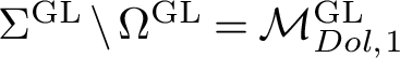

Remark 4.1. Observe that in both cases all of the strata satisfy the equality
 $$ \begin{align*} k=\dfrac{1}{2}(\dim\tilde{\mathcal{M}}_{Dol}^G-\mathcal{M}^G_{Dol,k}); \end{align*} $$
that is, they are relevant strata in the decomposition theorem for
 $\tilde {\pi }^G$
.
$\tilde {\pi }^G$
.
4.3 Decomposition theorem for
$\tilde {\pi }^G$

We have constructed a semismall desingularisation
 $\tilde {\mathcal {M}}_{Dol}^G\xrightarrow {\tilde {\pi }^{G}} \mathcal {M}_{Dol}^G$
. As seen in the proof of Proposition (4.3), all of the strata of the map
$\tilde {\mathcal {M}}_{Dol}^G\xrightarrow {\tilde {\pi }^{G}} \mathcal {M}_{Dol}^G$
. As seen in the proof of Proposition (4.3), all of the strata of the map
 $\tilde {\pi }^{G}:\tilde {\mathcal {M}}_{Dol}^{G}\rightarrow \mathcal {M}_{Dol}^G$
are relevant. In particular,
$\tilde {\pi }^{G}:\tilde {\mathcal {M}}_{Dol}^{G}\rightarrow \mathcal {M}_{Dol}^G$
are relevant. In particular,
 $$ \begin{align*} \mathcal{M}_{Dol}^{G,s}=\mathcal{M}^{G}_{Dol,0}, \quad \Sigma^{G}=\mathcal{M}^{G}_{Dol,1}, \quad \Omega^{G}=\mathcal{M}^{G}_{Dol,3}. \end{align*} $$
Stratify
 $\tilde {\mathcal {M}}_{Dol}^G$
as follows:
$\tilde {\mathcal {M}}_{Dol}^G$
as follows:
 $$ \begin{align*} \tilde{\mathcal{M}}_{Dol}^{G}=(\tilde{\pi}^{G})^{-1}(\mathcal{M}_{Dol}^{G,s})\sqcup (\tilde{\Sigma}^{G}\setminus \tilde{\Omega}^{G})\sqcup \tilde{\Omega}^{G}, \end{align*} $$
where
 $\tilde {\Sigma }^{G}:=(\tilde {\pi }^{G})^{-1}(\Sigma )$
and
$\tilde {\Sigma }^{G}:=(\tilde {\pi }^{G})^{-1}(\Sigma )$
and
 $\tilde {\Omega }^{G}:=(\tilde {\pi }^{G})^{-1}(\Omega ^G)$
.
$\tilde {\Omega }^{G}:=(\tilde {\pi }^{G})^{-1}(\Omega ^G)$
.
By the decomposition theorem, one obtains the splitting
 $$ \begin{align} IC_{\tilde{\mathcal{M}}_{Dol}^{G}}=IC_{\mathcal{M}_{Dol}^{G}}(\mathcal{L}_{\mathcal{M}_{Dol}^{G}})\oplus IC_{\Sigma^{G}}(\mathcal{L}_{\Sigma^{G}})\oplus IC_{\Omega^{G}}(\mathcal{L}_{\Omega^{G}}). \end{align} $$
Notice that, up to dimensional shifts, the stalks of the local systems
 $\mathcal {L}_{\Sigma ^{G}}$
and
$\mathcal {L}_{\Sigma ^{G}}$
and
 $\mathcal {L}_{\Omega ^{G}}$
in a generic point of the corresponding stratum are isomorphic to the top cohomology groups of the fibres, which are, respectively,
$\mathcal {L}_{\Omega ^{G}}$
in a generic point of the corresponding stratum are isomorphic to the top cohomology groups of the fibres, which are, respectively,
 $H^2(\mathbb {P}^1)$
and
$H^2(\mathbb {P}^1)$
and
 $H^6(\mathcal {G})$
. Moreover, because the fibres of
$H^6(\mathcal {G})$
. Moreover, because the fibres of
 $\tilde {\pi }^{G}$
over
$\tilde {\pi }^{G}$
over
 $\Sigma ^G$
and
$\Sigma ^G$
and
 $\Omega ^G$
are irreducible, the monodromy of
$\Omega ^G$
are irreducible, the monodromy of
 $\mathcal {L}_{\Sigma ^{G}}$
and
$\mathcal {L}_{\Sigma ^{G}}$
and
 $\mathcal {L}_{\Omega ^{G}}$
is trivial. Finally, because
$\mathcal {L}_{\Omega ^{G}}$
is trivial. Finally, because
 $\Omega ^G$
is nonsingular and
$\Omega ^G$
is nonsingular and
 $\Sigma ^G$
has finite quotient singularities, intersection cohomology and cohomology coincide. One has
$\Sigma ^G$
has finite quotient singularities, intersection cohomology and cohomology coincide. One has
 $$ \begin{align*} IC_{\mathcal{M}_{Dol}}(\mathcal{L}_{\mathcal{M}_{Dol}})_{\mid\mathcal{M}_{Dol}^s}&=\mathbb{Q}[\dim \mathcal{M}_{Dol}^G],\quad\, IC_{\Sigma}(\mathcal{L}_{\Sigma})\cong \mathbb{Q}[\dim \Sigma^G](-1),\\ IC_{\Omega}(\mathcal{L}_{\Omega})&\cong\mathbb{Q}[\dim \Omega^{G}](-3), \end{align*} $$
where the Tate shifts
 $(-1)$
and
$(-1)$
and
 $(-3)$
correspond to the Hodge structures
$(-3)$
correspond to the Hodge structures
 $\mathbb {Q}(-1)$
of
$\mathbb {Q}(-1)$
of
 $H^2(\mathbb {P}^1)$
and
$H^2(\mathbb {P}^1)$
and
 $\mathbb {Q}(-3)$
of
$\mathbb {Q}(-3)$
of
 $H^6(\mathcal {G})$
.
$H^6(\mathcal {G})$
.
Taking hypercohomology on both sides of (7), one has
 $$ \begin{align} H^*(\tilde{\mathcal{M}}_{Dol}^G)=IH^*(\mathcal{M}_{Dol}^G)\oplus H^{*-2}(\Sigma^G)(-1)\oplus H^{*-6}(\Omega^G)(-3). \end{align} $$
5 Purity of the Hodge structure
The aim of this section is to show that, although
 $\tilde {\mathcal {M}}_{Dol}^G$
is noncompact, the Hodge structure on its cohomology is pure; that is,
$\tilde {\mathcal {M}}_{Dol}^G$
is noncompact, the Hodge structure on its cohomology is pure; that is,
 $H^k(\tilde {\mathcal {M}}_{Dol}^G)$
has weight k for any
$H^k(\tilde {\mathcal {M}}_{Dol}^G)$
has weight k for any
 $k=0\ldots 2\dim \tilde {\mathcal {M}}_{Dol}^G$
.
$k=0\ldots 2\dim \tilde {\mathcal {M}}_{Dol}^G$
.
Recall that there exists the natural
 $\mathbb {C}^*$
action on
$\mathbb {C}^*$
action on
 $\mathcal {M}_{Dol}^G$
by scalar multiplication on the Higgs field
$\mathcal {M}_{Dol}^G$
by scalar multiplication on the Higgs field
 $\Phi $
. The Hitchin map
$\Phi $
. The Hitchin map
 $$ \begin{align*} \chi:\mathcal{M}_{Dol}^G\rightarrow \mathbb{A}=H^0(K_C)\oplus H^0(K^2_C) \end{align*} $$
is equivariant with respect to this action if we let
 $\mathbb {C}^*$
act on
$\mathbb {C}^*$
act on
 $H^0(C,K_C^{i})$
with weight i.
$H^0(C,K_C^{i})$
with weight i.
The following localisation result appears in several variants (e.g., [Reference Denef and Loeser12, Lemma 6.5] or [Reference De Cataldo, Migliorini and Mustăta9, Lemma 4.2]).
Lemma 5.1. Let
 $\rho :\mathbb {C}^*\times \mathbb {A}^n\rightarrow \mathbb {A}^n$
be a linear action on an affine space such that all of the weights of the action are positive. Denote by
$\rho :\mathbb {C}^*\times \mathbb {A}^n\rightarrow \mathbb {A}^n$
be a linear action on an affine space such that all of the weights of the action are positive. Denote by
 $s_0:\mathrm {Spec}\mathbb {C}\rightarrow \mathbb {A}^n$
the inclusion of the origin in
$s_0:\mathrm {Spec}\mathbb {C}\rightarrow \mathbb {A}^n$
the inclusion of the origin in
 $\mathbb {A}^n$
and by
$\mathbb {A}^n$
and by
 $p:\mathbb {A}^n\rightarrow \mathrm {Spec}\mathbb {C}$
the projection. Then for any
$p:\mathbb {A}^n\rightarrow \mathrm {Spec}\mathbb {C}$
the projection. Then for any
 $\mathbb {C}^*$
-equivariant complex K of sheaves on
$\mathbb {C}^*$
-equivariant complex K of sheaves on
 $\mathbb {A}^n$
one has
$\mathbb {A}^n$
one has
 $$ \begin{align*} Rp_*K=s_0^*K \text{ and } Rp_!K=s_0^!K. \end{align*} $$
As a corollary, one has the following result.
Proposition 5.2. Let X be a smooth variety with an action of
 $\mathbb {C}^*$
. Assume that
$\mathbb {C}^*$
. Assume that
 $f:X\rightarrow \mathbb {A}^n$
is a proper map, equivariant with respect to a linear action of
$f:X\rightarrow \mathbb {A}^n$
is a proper map, equivariant with respect to a linear action of
 $\mathbb {C}^*$
on the affine space
$\mathbb {C}^*$
on the affine space
 $\mathbb {A}^n$
, such that all of the weights of this action are positive. Let
$\mathbb {A}^n$
, such that all of the weights of this action are positive. Let
 $X_0:=f^{-1}(0)$
be the fibre of f over
$X_0:=f^{-1}(0)$
be the fibre of f over
 $0=\mathrm {Spec}\mathbb {C}\subset \mathbb {A}^n$
. Then there is an isomorphism of mixed Hodge structures
$0=\mathrm {Spec}\mathbb {C}\subset \mathbb {A}^n$
. Then there is an isomorphism of mixed Hodge structures
 $$ \begin{align*}H^*(X,\mathbb{Q})\cong H^*(X_0,\mathbb{Q}). \end{align*} $$
Proof. Because f is
 $\mathbb {C}^*$
-equivariant, we can apply Lemma 5.1 to
$\mathbb {C}^*$
-equivariant, we can apply Lemma 5.1 to
 $K=Rf_*\mathbb {Q}$
and by base change theorem for proper maps we get
$K=Rf_*\mathbb {Q}$
and by base change theorem for proper maps we get
 $$ \begin{align*}H^*(X,\mathbb{Q})\cong H^*(\mathbb{A}^n,Rf_*\mathbb{Q})\cong H^*(\mathrm{Spec}\mathbb{C},s_0^*Rf_*\mathbb{Q})\cong H^*(X_0,\mathbb{Q}).\end{align*} $$
For smooth moduli spaces
 $\mathcal {M}_{Dol}(d,n)$
of Higgs bundles of coprime rank and degree, the variety
$\mathcal {M}_{Dol}(d,n)$
of Higgs bundles of coprime rank and degree, the variety
 $X_0:=\chi ^{-1}(0)$
is the nilpotent cone of
$X_0:=\chi ^{-1}(0)$
is the nilpotent cone of
 $\chi $
and the previous proposition yields the purity of the Hodge structure on cohomology groups of those moduli spaces. In fact, on the one hand,
$\chi $
and the previous proposition yields the purity of the Hodge structure on cohomology groups of those moduli spaces. In fact, on the one hand,
 $\mathcal {M}_{Dol}(d,n)$
is smooth, so by the weight restrictions in Remark 2.2 the weights of
$\mathcal {M}_{Dol}(d,n)$
is smooth, so by the weight restrictions in Remark 2.2 the weights of
 $H^k(\mathcal {M}_{Dol}(d,n))$
are
$H^k(\mathcal {M}_{Dol}(d,n))$
are
 $\geq k$
. On the other hand, Proposition 5.2 gives an isomorphism of mixed Hodge structures between the cohomology of
$\geq k$
. On the other hand, Proposition 5.2 gives an isomorphism of mixed Hodge structures between the cohomology of
 $\mathcal {M}_{Dol}(d,n)$
and that of the nilpotent cone, which is compact; thus, the weights of
$\mathcal {M}_{Dol}(d,n)$
and that of the nilpotent cone, which is compact; thus, the weights of
 $H^k(\mathcal {M}_{Dol}(d,n))$
are
$H^k(\mathcal {M}_{Dol}(d,n))$
are
 $\leq k$
. Combining these two conditions, one has that
$\leq k$
. Combining these two conditions, one has that
 $H^k(\mathcal {M}_{Dol}(d,n))$
has weight k.
$H^k(\mathcal {M}_{Dol}(d,n))$
has weight k.
Let
 $\tilde {\chi }:\tilde {\mathcal {M}}_{Dol}^G\rightarrow \mathbb {A}$
be the composition of
$\tilde {\chi }:\tilde {\mathcal {M}}_{Dol}^G\rightarrow \mathbb {A}$
be the composition of
 $\chi $
with
$\chi $
with
 $\tilde {\pi }^G$
. Suppose that one can extend the
$\tilde {\pi }^G$
. Suppose that one can extend the
 $\mathbb {C}^*$
action on
$\mathbb {C}^*$
action on
 $\mathcal {M}_{Dol}^G$
to
$\mathcal {M}_{Dol}^G$
to
 $\tilde {\mathcal {M}}_{Dol}^G$
in a way such that
$\tilde {\mathcal {M}}_{Dol}^G$
in a way such that
 $\tilde {\chi }$
is equivariant. Because
$\tilde {\chi }$
is equivariant. Because
 $\tilde {\chi }$
is a proper map, the variety
$\tilde {\chi }$
is a proper map, the variety
 $\tilde {\chi }^{-1}(0)$
is compact. As a result, the above weight trick applies to
$\tilde {\chi }^{-1}(0)$
is compact. As a result, the above weight trick applies to
 $\tilde {\mathcal {M}}_{Dol}^G$
as well proving the following result.
$\tilde {\mathcal {M}}_{Dol}^G$
as well proving the following result.
Theorem 5.3. Let
 $\tilde {\mathcal {M}}_{Dol}^G$
be the semismall desingularisation of
$\tilde {\mathcal {M}}_{Dol}^G$
be the semismall desingularisation of
 $\mathcal {M}_{Dol}^G$
constructed in Section 4. Then the Hodge structure on
$\mathcal {M}_{Dol}^G$
constructed in Section 4. Then the Hodge structure on
 $H^*(\tilde {\mathcal {M}}_{Dol}^G)$
is pure.
$H^*(\tilde {\mathcal {M}}_{Dol}^G)$
is pure.
Moreover, as a consequence of the decomposition theorem, the Hodge structure on
 $IH^*(\mathcal {M}_{Dol}^G)$
is a sub-Hodge structure of that on
$IH^*(\mathcal {M}_{Dol}^G)$
is a sub-Hodge structure of that on
 $H^*(\tilde {\mathcal {M}}_{Dol}^G)$
, so the former is pure whenever the latter is.
$H^*(\tilde {\mathcal {M}}_{Dol}^G)$
, so the former is pure whenever the latter is.
Corollary 5.4. The Hodge structure on
 $IH^*(\mathcal {M}_{Dol}^G)$
is pure.
$IH^*(\mathcal {M}_{Dol}^G)$
is pure.
The above considerations reduce the proof of Theorem 5.3 to showing the following lemma.
Lemma 5.5. There exists a
 $\mathbb {C}^*$
action on
$\mathbb {C}^*$
action on
 $\tilde {\mathcal {M}}_{Dol}^G$
extending the natural
$\tilde {\mathcal {M}}_{Dol}^G$
extending the natural
 $\mathbb {C}^*$
action on
$\mathbb {C}^*$
action on
 $\mathcal {M}_{Dol}^G$
with respect to which the map
$\mathcal {M}_{Dol}^G$
with respect to which the map
 $\tilde {\chi }$
is equivariant.
$\tilde {\chi }$
is equivariant.
Proof. Because
 $\tilde {\pi }^G:\tilde {\mathcal {M}}_{Dol}^G\rightarrow \mathcal {M}_{Dol}^G$
is an isomorphism on the smooth locus, to prove the lemma one needs to extend the
$\tilde {\pi }^G:\tilde {\mathcal {M}}_{Dol}^G\rightarrow \mathcal {M}_{Dol}^G$
is an isomorphism on the smooth locus, to prove the lemma one needs to extend the
 $\mathbb {C}^*$
action to the fibres of
$\mathbb {C}^*$
action to the fibres of
 $\tilde {\pi }^G$
over the singular loci.
$\tilde {\pi }^G$
over the singular loci.
Given a point
 $v=(V,\Phi )\in \mathcal {M}_{Dol}^G$
,
$v=(V,\Phi )\in \mathcal {M}_{Dol}^G$
,
 $T_v\mathcal {M}_{Dol}^G\cong T^1{\mathbin{/\mkern-5.5mu/}} \mathrm {Stab}(v)$
, where
$T_v\mathcal {M}_{Dol}^G\cong T^1{\mathbin{/\mkern-5.5mu/}} \mathrm {Stab}(v)$
, where
 $T^1=\mathrm {Ext}^1_H(V,V)$
. By construction, the fibre of
$T^1=\mathrm {Ext}^1_H(V,V)$
. By construction, the fibre of
 $\tilde {\pi }^G$
over
$\tilde {\pi }^G$
over
 $\Sigma ^G$
(respectively
$\Sigma ^G$
(respectively
 $\Omega ^G)$
is the fibre of the normal cone
$\Omega ^G)$
is the fibre of the normal cone
 $C_{\Sigma }\mathcal {M}_{Dol}^G$
to
$C_{\Sigma }\mathcal {M}_{Dol}^G$
to
 $\Sigma ^G$
(respectively
$\Sigma ^G$
(respectively
 $\Omega ^G)$
in
$\Omega ^G)$
in
 $\mathcal {M}_{Dol}^G$
. Recall that by Proposition 3.5,
$\mathcal {M}_{Dol}^G$
. Recall that by Proposition 3.5,
 $$ \begin{align*} (C_\Sigma\mathcal{M}_{Dol}^G)_v\cong \overline\Upsilon^{-1}(0){\mathbin{/\mkern-5.5mu/}} \mathrm{Stab}(v) \end{align*} $$
for all
 $v\in \Sigma ^G$
(respectively
$v\in \Sigma ^G$
(respectively
 $\Omega ^G$
) and that
$\Omega ^G$
) and that
 $\overline \Upsilon ^{-1}(0)\subset T^1$
. As a consequence, to describe the action on the fibres one first needs to describe it over
$\overline \Upsilon ^{-1}(0)\subset T^1$
. As a consequence, to describe the action on the fibres one first needs to describe it over
 $T^1$
. Consider the diagram
$T^1$
. Consider the diagram

An element
 $\lambda \in \mathbb {C}^*$
acts on the diagram by scalar multiplication on the Higgs field in the commutator. Because
$\lambda \in \mathbb {C}^*$
acts on the diagram by scalar multiplication on the Higgs field in the commutator. Because
 $T^1\cong \operatorname {\mathrm {Im}} \alpha \oplus \mathrm {coker}\beta $
,
$T^1\cong \operatorname {\mathrm {Im}} \alpha \oplus \mathrm {coker}\beta $
,
 $\lambda \in \mathbb {C}^*$
acts on
$\lambda \in \mathbb {C}^*$
acts on
 $T^1$
as scalar multiplication on
$T^1$
as scalar multiplication on
 $ \operatorname {\mathrm {Im}} \alpha $
and as the identity on
$ \operatorname {\mathrm {Im}} \alpha $
and as the identity on
 $\mathrm {coker}\beta $
. Because both
$\mathrm {coker}\beta $
. Because both
 $\Sigma ^G$
and
$\Sigma ^G$
and
 $\Omega ^G$
are
$\Omega ^G$
are
 $\mathbb {C}^*$
-invariant, one can easily show that
$\mathbb {C}^*$
-invariant, one can easily show that
 $\overline {\Upsilon }^{-1}(0)$
is invariant under the
$\overline {\Upsilon }^{-1}(0)$
is invariant under the
 $\mathbb {C}^*$
action on
$\mathbb {C}^*$
action on
 $T^1$
. Moreover, such action commutes with that of the stabiliser, so one has a well-defined action on the fibres of
$T^1$
. Moreover, such action commutes with that of the stabiliser, so one has a well-defined action on the fibres of
 $\tilde {\pi }^G$
. Observe that by construction the map
$\tilde {\pi }^G$
. Observe that by construction the map
 $\tilde {\chi }$
is
$\tilde {\chi }$
is
 $\mathbb {C}^*$
-equivariant.
$\mathbb {C}^*$
-equivariant.
Purity of the Hodge structure on cohomology groups yields, by Poincaré duality, purity of Hodge structure on cohomology groups with compact supports. The following lemma implies that intersection Betti numbers of
 $\mathcal {M}_{Dol}^G$
and Betti numbers of
$\mathcal {M}_{Dol}^G$
and Betti numbers of
 $\tilde {\mathcal {M}}_{Dol}^G$
can be computed just by knowing E-polynomials.
$\tilde {\mathcal {M}}_{Dol}^G$
can be computed just by knowing E-polynomials.
Lemma 5.6. Let X be a complex algebraic variety, possibly singular, and let
 $$ \begin{align*} IE(X)=\sum_{p,q} \alpha^{p,q} u^pv^q \end{align*} $$
denote its intersection E-polynomial. If
 $IH^*(X)$
admits a pure Hodge structure, then
$IH^*(X)$
admits a pure Hodge structure, then
 $$ \begin{align*} ib_k(X):=\dim IH^k(X)=\sum_{p+q=2\dim X-k} \alpha^{p,q} \end{align*} $$
for any
 $k=0\ldots 2\dim X$
.
$k=0\ldots 2\dim X$
.
Remark 5.1. When X is nonsingular,
 $IH^*(X)=H^*(X)$
, so the formula in Lemma 5.6 holds for E-polynomial and usual Betti numbers.
$IH^*(X)=H^*(X)$
, so the formula in Lemma 5.6 holds for E-polynomial and usual Betti numbers.
Proof of Lemma 5.6. If
 $IH^*(X)$
admits a pure Hodge structure then,
$IH^*(X)$
admits a pure Hodge structure then,
 $IH^k(X)$
has weight k for any
$IH^k(X)$
has weight k for any
 $k=0\ldots 2\dim X$
. Recall that intersection cohomology groups satisfy Poincaré-Verdier duality
$k=0\ldots 2\dim X$
. Recall that intersection cohomology groups satisfy Poincaré-Verdier duality
 $$ \begin{align*} IH^k(X)\cong IH_c^{2\dim X-k}(X) \end{align*} $$
and that this isomorphism maps classes of type
 $(p,q)$
in classes of type
$(p,q)$
in classes of type
 $(\dim X-p,\dim X-q)$
. This concludes the proof.
$(\dim X-p,\dim X-q)$
. This concludes the proof.
5.1 Computation of the intersection E-polynomial
The aim of the next two sections is to compute the intersection E-polynomial
 $IE(\mathcal {M}_{Dol}^G)$
for
$IE(\mathcal {M}_{Dol}^G)$
for
 $G=\mathrm {SL}(2,\mathbb {C})$
and
$G=\mathrm {SL}(2,\mathbb {C})$
and
 $G=\mathrm {GL}(2,\mathbb {C})$
; as a consequence of Lemma 5.6, they will give the intersection Betti numbers of the corresponding moduli spaces of Higgs bundles. Before proceeding with computations, we shall describe the general strategy.
$G=\mathrm {GL}(2,\mathbb {C})$
; as a consequence of Lemma 5.6, they will give the intersection Betti numbers of the corresponding moduli spaces of Higgs bundles. Before proceeding with computations, we shall describe the general strategy.
Computing hypercohomology with compact support on both sides of (7), the splitting in the decomposition theorem becomes
 $$ \begin{align*} H_c^*(\tilde{\mathcal{M}}_{Dol}^G)=IH_c^*(\mathcal{M}_{Dol}^G) \oplus H_c^{*-2}(\Sigma^G)(-1)\oplus H_c^{*-6}(\Omega^G)(-3). \end{align*} $$
This equality holds also at the level of E-polynomials:
 $$ \begin{align} E(\tilde{\mathcal{M}}_{Dol}^{G})=IE(\mathcal{M}_{Dol}^G)+E^{top}(\tilde{\Sigma}^G)+E^{top}(\tilde{\Omega}^G), \end{align} $$
where
 $E^{top}(\tilde {\Sigma }^G)=E(\Sigma ^G\times H^2(\mathbb {P}^1))$
and
$E^{top}(\tilde {\Sigma }^G)=E(\Sigma ^G\times H^2(\mathbb {P}^1))$
and
 $E^{top}(\tilde {\Omega }^G)=E(\Omega ^G\times H^6(\mathcal {G}))$
.
$E^{top}(\tilde {\Omega }^G)=E(\Omega ^G\times H^6(\mathcal {G}))$
.
By additivity of E-polynomials,
 $E(\tilde {\mathcal {M}}_{Dol}^{G})$
is given by
$E(\tilde {\mathcal {M}}_{Dol}^{G})$
is given by
 $$ \begin{align} E(\tilde{\mathcal{M}}_{Dol}^{G})=E(\mathcal{M}_{Dol}^{G,s})+E(\tilde{\Sigma}^G\setminus \tilde{\Omega}^G)+E(\tilde{\Omega}^G). \end{align} $$
In order to obtain
 $IE(\mathcal {M}_{Dol}^G)$
, by (9) it is sufficient to subtract from
$IE(\mathcal {M}_{Dol}^G)$
, by (9) it is sufficient to subtract from
 $E(\tilde {\mathcal {M}}_{Dol}^{G})$
the contributions
$E(\tilde {\mathcal {M}}_{Dol}^{G})$
the contributions
 $E^{top}$
coming from the top cohomology of the fibres over the singular loci.
$E^{top}$
coming from the top cohomology of the fibres over the singular loci.
6 Intersection cohomology of
$\mathcal {M}_{Dol}^{\mathrm {SL}}$

Consider the semismall desingularisation
 $\tilde {\mathcal {M}}_{Dol}^{\mathrm {SL}}\xrightarrow {\tilde {\pi }^{\mathrm {SL}}} \mathcal {M}_{Dol}^{\mathrm {SL}}$
of the moduli space
$\tilde {\mathcal {M}}_{Dol}^{\mathrm {SL}}\xrightarrow {\tilde {\pi }^{\mathrm {SL}}} \mathcal {M}_{Dol}^{\mathrm {SL}}$
of the moduli space
 $\mathcal {M}_{Dol}^{\mathrm {SL}}$
of Higgs bundles of rank 2, degree 0 and trivial determinant over C. The aim of this subsection is to prove the following theorem.
$\mathcal {M}_{Dol}^{\mathrm {SL}}$
of Higgs bundles of rank 2, degree 0 and trivial determinant over C. The aim of this subsection is to prove the following theorem.
Theorem 6.1.
Intersection cohomology of
$\mathcal {M}_{Dol}^{\mathrm {SL}}$
The intersection Poincaré polynomial of
 $\mathcal {M}_{Dol}^{\mathrm {SL}}$
is
$\mathcal {M}_{Dol}^{\mathrm {SL}}$
is
 $$ \begin{align*} IP_t(\mathcal{M}_{Dol}^{\mathrm{SL}})=1+t^2+17t^4+17t^6. \end{align*} $$
Moreover, the Hodge diamond is
 $$ \begin{align*} \begin{array}{l|ccc} H^0&&\textit{(0,0)}&\\ &&&\\ H^2&&\textit{(1,1)}&\\ &&&\\ H^4&&\textit{17(2,2)}&\\ &&&\\ H^6&&\textit{17(3,3)}&\\ \end{array} \end{align*} $$
The proof of the theorem consists of computing the intersection E-polynomial
 $IE(\mathcal {M}_{Dol}^{\mathrm {SL}})$
and applying Lemma 5.6 to get intersection Betti numbers. By (9) one needs first to compute
$IE(\mathcal {M}_{Dol}^{\mathrm {SL}})$
and applying Lemma 5.6 to get intersection Betti numbers. By (9) one needs first to compute
 $E(\tilde {\mathcal {M}}_{Dol}^{\mathrm {SL}})$
using the stratification in (10).
$E(\tilde {\mathcal {M}}_{Dol}^{\mathrm {SL}})$
using the stratification in (10).
6.1 Cohomology of
$\mathcal {M}_{Dol}^{\mathrm {SL},s}$

Consider the smooth part
 $\mathcal {M}_{Dol}^{\mathrm {SL},s}$
of the moduli space
$\mathcal {M}_{Dol}^{\mathrm {SL},s}$
of the moduli space
 $\mathcal {M}_{Dol}^{\mathrm {SL}}$
, which parametrises stable pairs
$\mathcal {M}_{Dol}^{\mathrm {SL}}$
, which parametrises stable pairs
 $(V,\Phi )$
.
$(V,\Phi )$
.
Proposition 6.2. Let
 $\mathcal {M}_{Dol}^{\mathrm {SL},s}\subset \mathcal {M}_{Dol}^{\mathrm {SL}}$
be the locus of stable Higgs pairs. Then the E-polynomial of
$\mathcal {M}_{Dol}^{\mathrm {SL},s}\subset \mathcal {M}_{Dol}^{\mathrm {SL}}$
be the locus of stable Higgs pairs. Then the E-polynomial of
 $\mathcal {M}_{Dol}^{\mathrm {SL},s}$
is
$\mathcal {M}_{Dol}^{\mathrm {SL},s}$
is
 $$ \begin{align*} E(\mathcal{M}_{Dol}^{\mathrm{SL},s})=u^6v^6+u^5v^5+16u^4v^4+13u^3v^3-u^2v^4-u^4v^2-17u^2v^2. \end{align*} $$
It is well known that
 $\mathcal {M}_{Dol}^{\mathrm {SL},s}$
contains the cotangent bundle of the locus
$\mathcal {M}_{Dol}^{\mathrm {SL},s}$
contains the cotangent bundle of the locus
 $\mathcal {S}$
of stable vector bundles with trivial determinant as an open dense subset, but there are several stable Higgs bundles whose underlying vector bundle is not stable. This is due to the fact that not all vector subbundles of V are Higgs subbundles: for example, one may consider the bundle
$\mathcal {S}$
of stable vector bundles with trivial determinant as an open dense subset, but there are several stable Higgs bundles whose underlying vector bundle is not stable. This is due to the fact that not all vector subbundles of V are Higgs subbundles: for example, one may consider the bundle
 $$ \begin{align*} V=K_C^{-1}\oplus K_C, \end{align*} $$
where
 $K_C$
denotes the canonical bundle on X. This vector bundle is not stable because the subbundle
$K_C$
denotes the canonical bundle on X. This vector bundle is not stable because the subbundle
 $K_C$
has slope greater than the slope of V; however,
$K_C$
has slope greater than the slope of V; however,
 $K_C$
is not a Higgs subbundle because, in order for it to be
$K_C$
is not a Higgs subbundle because, in order for it to be
 $\Phi $
invariant,
$\Phi $
invariant,
 $Hom(K_C,K_C^{-1})\cong K_C^{-2}$
should have global sections, which is not the case because it has negative degree.
$Hom(K_C,K_C^{-1})\cong K_C^{-2}$
should have global sections, which is not the case because it has negative degree.
To determine the E-polynomial of
 $\mathcal {M}_{Dol}^{\mathrm {SL},s}$
, one constructs a suitable stratification, computes E-polynomials of all strata and sums them. In particular, because it is of its own interest, we also compute Betti numbers of the strata by systematic employment of the following well-known result.
$\mathcal {M}_{Dol}^{\mathrm {SL},s}$
, one constructs a suitable stratification, computes E-polynomials of all strata and sums them. In particular, because it is of its own interest, we also compute Betti numbers of the strata by systematic employment of the following well-known result.
Proposition 6.3. Addivity property of compact support cohomology
Let Y be a quasi-projective variety. Let Z be a closed subset of Y and call U its complement. Then, given the inclusions
, there is a long exact sequence in cohomology

We stratify the locus of stable Higgs pairs with respect to the stability of the underlying vector bundle:
-
• pairs
$(V,\Phi )$
with V stable vector bundle; -
• pairs
$(V,\Phi )$
with V strictly semistable vector bundle; -
• pairs
$(V,\Phi )$
with V unstable vector bundle.


6.2 The stable case
We shall parametrise all stable Higgs bundles
 $(V,\Phi )$
where V is a stable vector bundle.
$(V,\Phi )$
where V is a stable vector bundle.
Proposition 6.4. Let
 $\mathcal {S}$
be the locus of stable vector bundles with trivial determinant. The locus of stable Higgs pairs
$\mathcal {S}$
be the locus of stable vector bundles with trivial determinant. The locus of stable Higgs pairs
 $(V,\Phi )$
with
$(V,\Phi )$
with
 $V\in \mathcal {S}$
is isomorphic to
$V\in \mathcal {S}$
is isomorphic to
 $T^*\mathcal {S}$
and its E- polynomial is
$T^*\mathcal {S}$
and its E- polynomial is
 $$ \begin{align*} E(\mathcal{T}^*S)(u,v)=u^6v^6-u^3v^5-u^5v^3-3u^4v^4. \end{align*} $$
Proof. Clearly, if V is a stable vector bundle, then
 $(V,\Phi )$
is a stable Higgs pair. As a consequence, the locus of stable Higgs pairs with stable underlying vector bundle is isomorphic to
$(V,\Phi )$
is a stable Higgs pair. As a consequence, the locus of stable Higgs pairs with stable underlying vector bundle is isomorphic to
 $T^*\mathcal {S}$
. Narasimhan and Ramanan [Reference Narasimhan and Ramanan32] proved that the moduli space of semistable vector bundles with trivial determinant on a nonsingular projective curve C of genus 2 is isomorphic to
$T^*\mathcal {S}$
. Narasimhan and Ramanan [Reference Narasimhan and Ramanan32] proved that the moduli space of semistable vector bundles with trivial determinant on a nonsingular projective curve C of genus 2 is isomorphic to
 $\mathbb {P}^3$
. A semistable vector bundle V is nonstable if and only if it is of the form
$\mathbb {P}^3$
. A semistable vector bundle V is nonstable if and only if it is of the form
 $$ \begin{align*} V=L\oplus L^{-1},\quad L\in Jac(C); \end{align*} $$
therefore, strictly semistable vector bundles are parametrised by
 $\mathcal {K}:=Jac(C)/\mathbb {Z}_2$
, where
$\mathcal {K}:=Jac(C)/\mathbb {Z}_2$
, where
 $\mathbb {Z}_2$
acts as the involution
$\mathbb {Z}_2$
acts as the involution
 $L\mapsto L^{-1}$
. The variety
$L\mapsto L^{-1}$
. The variety
 $\mathcal {K}$
is a compact Kummer surface with 16 singularities, corresponding to the fixed points of the involution, whose desingularisation is a K3 surface obtained by blowing up
$\mathcal {K}$
is a compact Kummer surface with 16 singularities, corresponding to the fixed points of the involution, whose desingularisation is a K3 surface obtained by blowing up
 $\mathcal {K}$
in the singular points. As a result, the locus
$\mathcal {K}$
in the singular points. As a result, the locus
 $\mathcal {S}$
of stable bundles is the complement of
$\mathcal {S}$
of stable bundles is the complement of
 $\mathcal {K}$
inside
$\mathcal {K}$
inside
 $\mathbb {P}^3$
.
$\mathbb {P}^3$
.
Observe that the cohomology of
 $\mathcal {K}$
is the
$\mathcal {K}$
is the
 $\mathbb {Z}_2$
-invariant part of the cohomology of
$\mathbb {Z}_2$
-invariant part of the cohomology of
 $Jac(C)$
. The cohomology of the Jacobian is generated by
$Jac(C)$
. The cohomology of the Jacobian is generated by
 $H^1(Jac(C))$
and the Betti numbers are
$H^1(Jac(C))$
and the Betti numbers are
 $$ \begin{align*} b_0=1\quad b_1=4 \quad b_2=6 \quad b_3=4 \quad b_4=1. \end{align*} $$
The action of
 $\mathbb {Z}_2$
on the cohomology sends every generator
$\mathbb {Z}_2$
on the cohomology sends every generator
 $\gamma $
of
$\gamma $
of
 $H^1$
in
$H^1$
in
 $-\gamma $
; thus, the even cohomology groups are all
$-\gamma $
; thus, the even cohomology groups are all
 $\mathbb {Z}_2$
-invariant, whereas the odd ones are never. As a result, the Betti numbers of
$\mathbb {Z}_2$
-invariant, whereas the odd ones are never. As a result, the Betti numbers of
 $\mathcal {K}$
are
$\mathcal {K}$
are
 $$ \begin{align*} b_0=1\quad b_1=0 \quad b_2=6 \quad b_3=0 \quad b_4=1. \end{align*} $$
Alternatively, one can notice that the cohomology of
 $\mathcal {K}$
differs from that of its desingularisation just in the
$\mathcal {K}$
differs from that of its desingularisation just in the
 $H^2$
part, which has in addition the contribution of the 16 exceptional divisors isomorphic to
$H^2$
part, which has in addition the contribution of the 16 exceptional divisors isomorphic to
 $\mathbb {P}^1$
, and the Betti numbers of a K3 surface are
$\mathbb {P}^1$
, and the Betti numbers of a K3 surface are
 $$ \begin{align*} b_0=1\quad b_1=0 \quad b_2=22 \quad b_3=0 \quad b_4=1. \end{align*} $$
Observe that because the Hodge structure on the cohomology of
 $Jac(C)$
is pure, so is the cohomology of
$Jac(C)$
is pure, so is the cohomology of
 $\mathcal {K}$
. In particular,
$\mathcal {K}$
. In particular,
 $ H^0(\mathcal {K})$
has weight 0,
$ H^0(\mathcal {K})$
has weight 0,
 $H^2(\mathcal {K})$
has weight 2 and types
$H^2(\mathcal {K})$
has weight 2 and types
 $4(1,1)+(2,0)+(0,2)$
and
$4(1,1)+(2,0)+(0,2)$
and
 $H^4(\mathcal {K})$
have weight 4 of type
$H^4(\mathcal {K})$
have weight 4 of type
 $(2,2)$
. Consider now the inclusions
$(2,2)$
. Consider now the inclusions
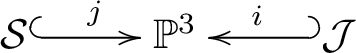
. Because both
 $\mathbb {P}^3$
and
$\mathbb {P}^3$
and
 $\mathcal {K}$
are compact, we have the long exact sequence:
$\mathcal {K}$
are compact, we have the long exact sequence:

which splits in the following sequences:


First consider (11): the map
 $i^{!}=i^*$
is a restriction to a hyperplane sections; therefore, it is an isomorphism by Lefschetz hyperplane theorem and
$i^{!}=i^*$
is a restriction to a hyperplane sections; therefore, it is an isomorphism by Lefschetz hyperplane theorem and
 $H_c^0(\mathcal {S})=H_c^1(\mathcal {S})=0$
.
$H_c^0(\mathcal {S})=H_c^1(\mathcal {S})=0$
.
For (12),
 $i^{!}$
is the restriction of the fundamental class of
$i^{!}$
is the restriction of the fundamental class of
 $\mathbb {P}^1$
inside
$\mathbb {P}^1$
inside
 $\mathbb {P}^2$
, which remains nonzero when intersecting it generically with
$\mathbb {P}^2$
, which remains nonzero when intersecting it generically with
 $\mathcal {K}$
, so
$\mathcal {K}$
, so
 $i^{!}$
is an injection. One has
$i^{!}$
is an injection. One has
 $H^2_c(\mathcal {S})=0$
and
$H^2_c(\mathcal {S})=0$
and
 $H^3_c(\mathcal {S})=\mathbb {C}^5$
. A similar argument shows that, in (13),
$H^3_c(\mathcal {S})=\mathbb {C}^5$
. A similar argument shows that, in (13),
 $i^{!}$
is an isomorphism and that
$i^{!}$
is an isomorphism and that
 $H_c^4(\mathcal {S})=H_c^5(\mathcal {S})=0$
.
$H_c^4(\mathcal {S})=H_c^5(\mathcal {S})=0$
.
Clearly, (14) shows that
 $H^6_c(\mathcal {S})\cong \mathbb {C}$
. By Poincaré duality, the Betti numbers are
$H^6_c(\mathcal {S})\cong \mathbb {C}$
. By Poincaré duality, the Betti numbers are
 $$ \begin{align*} b_0=1\quad b_1=0 \quad b_2=0 \quad b_3=5 \quad b_4=0 \quad b_5=0 \quad b_6=0. \end{align*} $$
Because
 $T^*\mathcal {S}$
is a vector bundle over
$T^*\mathcal {S}$
is a vector bundle over
 $\mathcal {S}$
, it inherits the cohomology of its base space, so the compact support cohomology groups of
$\mathcal {S}$
, it inherits the cohomology of its base space, so the compact support cohomology groups of
 $T^*\mathcal {S}$
are
$T^*\mathcal {S}$
are
 $$ \begin{align*} H^9_c(T^*\mathcal{S})&=5 \quad \text{of types }(3,5)+(5,3)+3(4,4)\\ H^{12}_c(T^*\mathcal{S})&=1 \quad \text{of type }(6,6)\\ H^i_c(T^*\mathcal{S})&=0 \quad \text{otherwise.} \end{align*} $$
As a result, the E-polynomial of Higgs bundles with stable underlying vector bundle is
 $$ \begin{align*} E(T^*\mathcal{S})(u,v)=u^6v^6-u^3v^5-u^5v^3-3u^4v^4. \end{align*} $$
6.3 Strictly semistable case
Suppose that V is a strictly semistable vector bundle. We would like to investigate when V occurs in a stable Higgs pair
 $(V,\Phi )$
. Again, one has to distinguish different cases:
$(V,\Phi )$
. Again, one has to distinguish different cases:
-
(i)
$V=L\oplus L^{-1}$
where
$L\in Jac(C)$
and
$L\not \cong L^{-1}$
. -
(ii)
$V$
is a nontrivial extension
with
$L\not \cong L^{-1}$
. -
(iii)
$V=L\oplus L$
where
$L\in Jac(C)$
and
$L\cong L^{-1}$
. -
(iv)
$V$
is a nontrivial extension
with
$L\cong L^{-1}$
.


6.3.1 Type
$\mathrm {(i)}$

We shall determine stable Higgs pairs having underlying vector bundle of
 $V=L\oplus L^{-1}$
with
$V=L\oplus L^{-1}$
with
 $L\in Jac(C)$
such that
$L\in Jac(C)$
such that
 $L\not \cong L^{-1}$
. Vector bundles of this form are parametrised by
$L\not \cong L^{-1}$
. Vector bundles of this form are parametrised by
 $\mathcal {K}=Jac(C)/\mathbb {Z}_2$
. We denote by
$\mathcal {K}=Jac(C)/\mathbb {Z}_2$
. We denote by
 $\mathcal {K}_0$
locus in
$\mathcal {K}_0$
locus in
 $\mathcal {K}$
fixed by the involution and by
$\mathcal {K}$
fixed by the involution and by
 $\mathcal {K}^0:=\mathcal {K}-\mathcal {K}_0$
its complement. Then the locus of stable Higgs bundles with underlying vector bundle of type (i) is a fibre bundle over
$\mathcal {K}^0:=\mathcal {K}-\mathcal {K}_0$
its complement. Then the locus of stable Higgs bundles with underlying vector bundle of type (i) is a fibre bundle over
 $\mathcal {K}^0$
.
$\mathcal {K}^0$
.
Proposition 6.5. Let
 $\mathcal {S}_1$
be the locus of stable Higgs bundles with underlying vector bundle of type
$\mathcal {S}_1$
be the locus of stable Higgs bundles with underlying vector bundle of type
 $\mathrm {(i)}$
. Then
$\mathrm {(i)}$
. Then
 $\mathcal {S}_1$
is a
$\mathcal {S}_1$
is a
 $(\mathbb {C}^2\times \mathbb {C}^*)$
-bundle over
$(\mathbb {C}^2\times \mathbb {C}^*)$
-bundle over
 $\mathcal {K}^0$
and its E-polynomial is
$\mathcal {K}^0$
and its E-polynomial is
 $$ \begin{align*} E(\mathcal{S}_1)(u,v)=u^5v^5+u^3v^5+u^5v^3+3u^4v^4-19u^3v^3-u^2v^4-u^4v^2+15 u^2v^2. \end{align*} $$
Proof. Consider
 $V=L\oplus L^{-1}$
with
$V=L\oplus L^{-1}$
with
 $L\in Jac(C)$
such that
$L\in Jac(C)$
such that
 $L\not \cong L^{-1}$
. We have that
$L\not \cong L^{-1}$
. We have that
 $$ \begin{align*} H^0(End_0(V)\otimes K_C)= H^0(K_C)\oplus H^0(L^2K_C)\oplus H^0(L^{-2}K_C); \end{align*} $$
thus, a Higgs field
 $\Phi \in H^0(End_0(V)\otimes K_C)$
will be of the form
$\Phi \in H^0(End_0(V)\otimes K_C)$
will be of the form
 $$ \begin{align*}\Phi=\left( \begin{array}{cc} a&b\\ c&-a\\ \end{array}\right)\end{align*} $$
with
 $a\in H^0(K_C)$
,
$a\in H^0(K_C)$
,
 $b\in H^0(L^2K_C)$
,
$b\in H^0(L^2K_C)$
,
 $c\in H^0(L^{-2}K_C)$
. A pair
$c\in H^0(L^{-2}K_C)$
. A pair
 $(V,\Phi )$
is stable if and only if both L and
$(V,\Phi )$
is stable if and only if both L and
 $L^{-1}$
are not preserved by
$L^{-1}$
are not preserved by
 $\Phi $
; that is,
$\Phi $
; that is,
 $b,c\neq 0$
. Then one needs to understand when two different Higgs fields give rise to isomorphic Higgs bundles: because the automorphism group of V is
$b,c\neq 0$
. Then one needs to understand when two different Higgs fields give rise to isomorphic Higgs bundles: because the automorphism group of V is
 $\mathbb {C}^*$
, two Higgs pairs
$\mathbb {C}^*$
, two Higgs pairs
 $(V,\Phi _1)$
and
$(V,\Phi _1)$
and
 $(V,\Phi _2)$
with
$(V,\Phi _2)$
with
 $\Phi _i=(a_i,b_i,c_i)$
are isomorphic if and only if
$\Phi _i=(a_i,b_i,c_i)$
are isomorphic if and only if
 $$ \begin{align*} \Phi_1=\left( \begin{array}{cc} t&0\\ 0&t^{-1}\\ \end{array}\right)\Phi_2\left( \begin{array}{cc} t^{-1}&0\\ 0&t\\ \end{array}\right);\end{align*} $$
that is,
 $a_1=a_2$
,
$a_1=a_2$
,
 $b_1=t^2 b_2$
,
$b_1=t^2 b_2$
,
 $c_1=t^{-2}c_2$
. Therefore, stable Higgs pairs
$c_1=t^{-2}c_2$
. Therefore, stable Higgs pairs
 $(V,\Phi )$
with fixed underline vector bundle V are parametrised by
$(V,\Phi )$
with fixed underline vector bundle V are parametrised by
 $$ \begin{align*} H^0(K_C)\times \dfrac{(H^0(L^2K)-\{0\})\times (H^0(L^{-2}K_C)-\{0\})}{\mathbb{C}^*} \cong\mathbb{C}^2\times \mathbb{C}^*. \end{align*} $$
This is an actual quotient because all of the points are semistable with respect to the action of
 $\mathbb {C}^*$
.
$\mathbb {C}^*$
.
Letting V vary, one obtains a
 $(\mathbb {C}^2\times \mathbb {C}^*)$
-bundle
$(\mathbb {C}^2\times \mathbb {C}^*)$
-bundle
 $\mathcal {S}_1$
over
$\mathcal {S}_1$
over
 $\mathcal {K}^0$
. Considering
$\mathcal {K}^0$
. Considering
 $\mathcal {S}_1$
as a sphere bundle over
$\mathcal {S}_1$
as a sphere bundle over
 $\mathcal {K}^0$
, the cohomology of the total space is computed by Gysin sequence. Consider the inclusions
$\mathcal {K}^0$
, the cohomology of the total space is computed by Gysin sequence. Consider the inclusions
and the long exact sequence in cohomology

which splits in

Because
 $\mathcal {K}^0$
is not compact,
$\mathcal {K}^0$
is not compact,
 $H^0_c(\mathcal {K}^0)=0$
, so
$H^0_c(\mathcal {K}^0)=0$
, so
 $H^1_c(\mathcal {K}^0)\cong \mathbb {C}^{15}$
. By Poincaré duality,
$H^1_c(\mathcal {K}^0)\cong \mathbb {C}^{15}$
. By Poincaré duality,
 $$ \begin{align*} H^0(\mathcal{K}^0)\cong\mathbb{C}\quad H^1(\mathcal{K}^0)=0\quad H^2(\mathcal{K}^0)=\mathbb{C}^6\quad H^3(\mathcal{K}^0)=\mathbb{C}^{15}\quad H^4(\mathcal{K}^0)=0 \end{align*} $$
with the same weights as the cohomology of
 $\mathcal {K}$
.
$\mathcal {K}$
.
The Gysin sequence
splits in the following subsequences:
 $$ \begin{align} H^0(\mathcal{S}_1)\cong \mathbb{C} \quad H^3(\mathcal{S}_1)\cong\mathbb{C}^{21} \quad H^{4}(\mathcal{S}_1)\cong\mathbb{C}^{15}; \end{align} $$
 $$ \begin{align} H^i(\mathcal{S}_1)=0\quad \forall i\geq 5. \end{align} $$
In (16) the map
 $\mathbb {C}\rightarrow \mathbb {C}^6$
is the product by the Euler class of a nontrivial bundle, which is nonzero; therefore,
$\mathbb {C}\rightarrow \mathbb {C}^6$
is the product by the Euler class of a nontrivial bundle, which is nonzero; therefore,
 $H^1(\mathcal {S}_1)=0$
and
$H^1(\mathcal {S}_1)=0$
and
 $H^2(\mathcal {S}_1)=\mathbb {C}^5$
. Recall that in this case both the cup product with the Euler class and the pushforward increase weights of (1,1). As a consequence of Poincaré duality, the compact support cohomology groups of
$H^2(\mathcal {S}_1)=\mathbb {C}^5$
. Recall that in this case both the cup product with the Euler class and the pushforward increase weights of (1,1). As a consequence of Poincaré duality, the compact support cohomology groups of
 $\mathcal {S}_1$
are
$\mathcal {S}_1$
are
 $$ \begin{align*} H^i_c(\mathcal{S}_1)&=0 &\forall i=0,\ldots 5 \text{ and }i=9&\quad\\ H^6_c(\mathcal{S}_1)&=\mathbb{C}^{15} & \text{ of type }(2,2)&\quad \\ H^7_c(\mathcal{S}_1)&=\mathbb{C}^{21} &\text{ of types }19(3,3)+(2,4)+(4,2)&\\ H^8_c(\mathcal{S}_1)&=\mathbb{C}^5 & \text{ of types }3(4,4)+(3,5)+(5,3)&\\ \quad H^{10}_c(\mathcal{S}_1)&=\mathbb{C} &\text{ of type }(5,5),& \end{align*} $$
and the E-polynomial of
 $\mathcal {S}_1$
is
$\mathcal {S}_1$
is
 $$ \begin{align*}E(\mathcal{S}_1)(u,v)=u^5v^5+u^3v^5+u^5v^3+3u^4v^4-19u^3v^3-u^2v^4-u^4v^2+15 u^2v^2.\end{align*} $$
6.3.2 Type
$\mathrm {(ii)}$

Now we want to compute the cohomology of the locus of stable pairs
 $(V,\Phi )$
where V is a nontrivial extension of L by
$(V,\Phi )$
where V is a nontrivial extension of L by
 $L^{-1}$
with
$L^{-1}$
with
 $L\not \cong L^{-1}$
.
$L\not \cong L^{-1}$
.
Proposition 6.6. Let V be a semistable vector bundle of type
 $\mathrm {(ii)}$
. Then there is no Higgs field
$\mathrm {(ii)}$
. Then there is no Higgs field
 $\Phi $
such that the pair
$\Phi $
such that the pair
 $(V,\Phi )$
is stable.
$(V,\Phi )$
is stable.
Proof. Consider the universal line bundle
 $\mathcal {L}\rightarrow \mathcal {K}^0\times C$
and let
$\mathcal {L}\rightarrow \mathcal {K}^0\times C$
and let
 $p:\mathcal {K}^0\times C \rightarrow \mathcal {K}^0$
be the projection onto the first factor. It is well known that nontrivial extensions of
$p:\mathcal {K}^0\times C \rightarrow \mathcal {K}^0$
be the projection onto the first factor. It is well known that nontrivial extensions of
 $\mathcal {L}$
by
$\mathcal {L}$
by
 $\mathcal {L}^{-1}$
are parametrised by
$\mathcal {L}^{-1}$
are parametrised by
 $\mathbb {P}(R^1p_{*}\mathcal {L}^2)$
: because
$\mathbb {P}(R^1p_{*}\mathcal {L}^2)$
: because
 $R^1p_{*}\mathcal {L}^2$
is a local system on
$R^1p_{*}\mathcal {L}^2$
is a local system on
 $\mathcal {K}^0$
of rank 1, there exists a unique nontrivial extension up to isomorphism. Consider the universal extension bundle
$\mathcal {K}^0$
of rank 1, there exists a unique nontrivial extension up to isomorphism. Consider the universal extension bundle
 $\mathcal {V}$
: it fits in the short exact sequence
$\mathcal {V}$
: it fits in the short exact sequence
 $$ \begin{align} 0\rightarrow \mathcal{L}\rightarrow \mathcal{V} \rightarrow \mathcal{L}^{-1}\rightarrow 0 \end{align} $$
and parametrises all of the vector bundles V on C of type (ii). In order for
 $(\mathcal {V},\Phi )$
to be a stable Higgs bundle, the Higgs field must not preserve the subbundle
$(\mathcal {V},\Phi )$
to be a stable Higgs bundle, the Higgs field must not preserve the subbundle
 $\mathcal {L}$
. By an abuse of notation, we denote by
$\mathcal {L}$
. By an abuse of notation, we denote by
 $K_C$
the pullback of the canonical bundle on C under the projection
$K_C$
the pullback of the canonical bundle on C under the projection
 $\mathcal {K}^0\times C\rightarrow C$
. Tensoring the sequence (18) by
$\mathcal {K}^0\times C\rightarrow C$
. Tensoring the sequence (18) by
 $K_C$
and applying the covariant functor
$K_C$
and applying the covariant functor
 $Hom(\mathcal {V},-)$
restricted to traceless endomorphisms gives
$Hom(\mathcal {V},-)$
restricted to traceless endomorphisms gives
 $$ \begin{align*}0\rightarrow Hom(\mathcal{V},\mathcal{L}\otimes K_C) \rightarrow End_0(\mathcal{V})\otimes K_C \rightarrow Hom(\mathcal{V},\mathcal{L}^{-1}\otimes K_C)\rightarrow 0.\end{align*} $$
Pushing forward to
 $\mathcal {K}^0$
gives a long exact sequence
$\mathcal {K}^0$
gives a long exact sequence

A Higgs pair
 $(\mathcal {V},\Phi )$
is stable if and only if the Higgs field
$(\mathcal {V},\Phi )$
is stable if and only if the Higgs field
 $\Phi $
lies in the complement of the kernel of the restriction map
$\Phi $
lies in the complement of the kernel of the restriction map
 $\rho : p_* End_0(\mathcal {V})\otimes K_C\rightarrow p_*\mathcal {L}^{-2}K_C$
. In order to prove the proposition, we show that
$\rho : p_* End_0(\mathcal {V})\otimes K_C\rightarrow p_*\mathcal {L}^{-2}K_C$
. In order to prove the proposition, we show that
 $\rho =0$
.
$\rho =0$
.
Applying the contravariant functor
 $p_*Hom(-,\mathcal {L} K_C)$
to (18) gives a long exact sequence
$p_*Hom(-,\mathcal {L} K_C)$
to (18) gives a long exact sequence

Consider the fibre of (20) on a point
 $L\in \mathcal {K}^0$
. One has
$L\in \mathcal {K}^0$
. One has
Because
 $H^1(L^2K_C)=0$
,
$H^1(L^2K_C)=0$
,
 $H^1(V^*LK_C)\cong H^1(K_C)\cong \mathbb {C}$
; thus,
$H^1(V^*LK_C)\cong H^1(K_C)\cong \mathbb {C}$
; thus,
 $R^1p_*Hom(\mathcal {V},\mathcal {L} K_C)$
is a local system of rank 1 on
$R^1p_*Hom(\mathcal {V},\mathcal {L} K_C)$
is a local system of rank 1 on
 $\mathcal {K}^0\times C$
. Now consider (19) in the fibre over
$\mathcal {K}^0\times C$
. Now consider (19) in the fibre over
 $L\in \mathcal {K}^0$
:
$L\in \mathcal {K}^0$
:

As seen before,
 $H^1(V^*LK_C)\cong H^1(K_C)\cong \mathbb {C}$
and
$H^1(V^*LK_C)\cong H^1(K_C)\cong \mathbb {C}$
and
 $H^0(L^{-2}K_C)\cong \mathbb {C}$
, so the map ext in (19) is either 0 or an isomorphism. However, because V is a nontrivial extension, such a map has to be nonzero; thus, it is an isomorphism. As a result,
$H^0(L^{-2}K_C)\cong \mathbb {C}$
, so the map ext in (19) is either 0 or an isomorphism. However, because V is a nontrivial extension, such a map has to be nonzero; thus, it is an isomorphism. As a result,
 $\rho $
is zero.
$\rho $
is zero.
6.3.3 Type
$\mathrm {(iii)}$

We consider stable Higgs bundles with underlying vector bundle
 $V=L\oplus L$
with
$V=L\oplus L$
with
 $L\cong L^{-1} \in \mathcal {K}_0$
.
$L\cong L^{-1} \in \mathcal {K}_0$
.
Proposition 6.7. Let
 $\textbf {S}_3$
be the locus of stable Higgs bundles with underlying vector bundle
$\textbf {S}_3$
be the locus of stable Higgs bundles with underlying vector bundle
 $V=\mathcal {O}\oplus \mathcal {O}$
. Then the locus
$V=\mathcal {O}\oplus \mathcal {O}$
. Then the locus
 $\mathcal {S}_3$
of stable Higgs pairs of type
$\mathcal {S}_3$
of stable Higgs pairs of type
 $\mathrm {(iii)}$
is the union of 16 copies of
$\mathrm {(iii)}$
is the union of 16 copies of
 $\textbf {S}_3$
and its E-polynomial is
$\textbf {S}_3$
and its E-polynomial is
 $$ \begin{align*} E(\mathcal{S}_3)(u,v)=16u^3v^3-16u^2v^2. \end{align*} $$
Proof. Up to tensor by
 $L\in \mathcal {K}_0$
one may restrict to the case,
$L\in \mathcal {K}_0$
one may restrict to the case,
 $L=\mathcal {O}$
, so that V is just the trivial bundle
$L=\mathcal {O}$
, so that V is just the trivial bundle
 $\mathcal {O}\oplus \mathcal {O}$
. In this case
$\mathcal {O}\oplus \mathcal {O}$
. In this case
 $H^0(\mathcal {E}nd_0(V)\otimes K_C)\cong H^0(K_C)\otimes sl(2)\cong \mathbb {C}^2\otimes sl(2)$
and the Higgs field is of the form
$H^0(\mathcal {E}nd_0(V)\otimes K_C)\cong H^0(K_C)\otimes sl(2)\cong \mathbb {C}^2\otimes sl(2)$
and the Higgs field is of the form
 $$ \begin{align*}\Phi=\left( \begin{array}{cc} a&b\\ c&-a\\ \end{array}\right) \text{ with } a,b,c\in H^0(K_C). \end{align*} $$
The bundle is not stable if and only if
 $\Phi $
is conjugate to an upper triangular matrix of elements of
$\Phi $
is conjugate to an upper triangular matrix of elements of
 $H^0(K_C)$
. Because the action of
$H^0(K_C)$
. Because the action of
 $\mathrm {SL}(2,\mathbb {C}) $
on
$\mathrm {SL}(2,\mathbb {C}) $
on
 $H^0(K_C)\otimes sl(2)$
is trivial on the first factor, one can consider
$H^0(K_C)\otimes sl(2)$
is trivial on the first factor, one can consider
 $\Phi \in H^0(K_C)\otimes sl(2) $
as a pair of matrices
$\Phi \in H^0(K_C)\otimes sl(2) $
as a pair of matrices
 $(A,B)\in sl(2)\oplus sl(2)$
on which
$(A,B)\in sl(2)\oplus sl(2)$
on which
 $\mathrm {SL}(2,\mathbb {C})$
acts by simultaneous conjugation. Then
$\mathrm {SL}(2,\mathbb {C})$
acts by simultaneous conjugation. Then
 $\Phi $
is conjugate to an upper triangular matrix of elements of
$\Phi $
is conjugate to an upper triangular matrix of elements of
 $H^0(K_C)$
if and only if A and B are simultaneously triangulable; that is, if they have a common eigenspace. By a result of Shemesh [Reference Shemesh38], this happens if and only if
$H^0(K_C)$
if and only if A and B are simultaneously triangulable; that is, if they have a common eigenspace. By a result of Shemesh [Reference Shemesh38], this happens if and only if
 $\ker [A,B]\neq 0$
; that is,
$\ker [A,B]\neq 0$
; that is,
 $\det ([A,B])=0$
. Writing
$\det ([A,B])=0$
. Writing
 $$ \begin{align} A=\left( \begin{array}{cc} x_1&x_2\\[-2pt] x_3&-x_1\\[-2pt] \end{array}\right)\qquad B=\left( \begin{array}{cc} y_1&y_2\\[-2pt] y_3&-y_1\\[-2pt] \end{array}\right)\end{align} $$
then
 $$ \begin{align*}[A,B]=\left( \begin{array}{cc} x_2y_3-y_2x_3&2(x_1y_2-x_2y_1)\\ 2(x_3y_1-x_1y_3)&-(x_2y_3-y_2x_3)\\ \end{array}\right).\end{align*} $$
One can interpret the locus of simultaneously triangulable matrices
 $(A,B)\in sl(2)\oplus sl(2)$
as a quartic hypersurface in
$(A,B)\in sl(2)\oplus sl(2)$
as a quartic hypersurface in
 $\mathbb {C}^6$
with coordinates
$\mathbb {C}^6$
with coordinates
 $(x_1,x_2,x_3,y_1,y_2,y_3)$
with the equation
$(x_1,x_2,x_3,y_1,y_2,y_3)$
with the equation
 $$ \begin{align*}Q: (x_2y_3-y_2x_3)^2+4(x_1y_2-x_2y_1)(x_3y_1-x_1y_3)=0,\end{align*} $$
given by annihilation of
 $\det [A,B]$
.
$\det [A,B]$
.
Lemma 6.8. A Higgs bundle
 $(V,\Phi )$
with
$(V,\Phi )$
with
 $V=\mathcal {O}\oplus \mathcal {O}$
is stable if and only if
$V=\mathcal {O}\oplus \mathcal {O}$
is stable if and only if
 $\Phi $
lies in
$\Phi $
lies in
 $$ \begin{align*} \textbf{S}_3:=(\mathbb{C}^6-Q){\mathbin{/\mkern-5.5mu/}} \mathrm{SL}(2,\mathbb{C}), \end{align*} $$
where
 $\mathrm {SL}(2,\mathbb {C})$
acts as the simultaneous conjugation on the matrices A and B as in (21).
$\mathrm {SL}(2,\mathbb {C})$
acts as the simultaneous conjugation on the matrices A and B as in (21).
Corollary 6.9. The locus of stable Higgs bundles of type
 $\mathrm {(iii)}$
is isomorphic to 16 copies of
$\mathrm {(iii)}$
is isomorphic to 16 copies of
 $\textbf {S}_3$
, one for each point of
$\textbf {S}_3$
, one for each point of
 $\mathcal {K}_0$
.
$\mathcal {K}_0$
.
Consider the quartic hypersurface Q in
 $\mathbb {C}^6$
. Setting
$\mathbb {C}^6$
. Setting
 $$ \begin{align*} \alpha &=x_2y_3-y_2x_3\\[-2pt] \beta &=x_1y_2-x_2y_1\\[-2pt] \gamma &=x_3y_1-x_1y_3, \end{align*} $$
then for every
 $(x_1,x_2,x_3,y_1,y_2,y_3)\in Q$
,
$(x_1,x_2,x_3,y_1,y_2,y_3)\in Q$
,
 $(\alpha ,\beta ,\gamma )$
satisfy the equation
$(\alpha ,\beta ,\gamma )$
satisfy the equation
 $$ \begin{align*} \alpha^2+4\beta\gamma=0. \end{align*} $$
This defines a map
 $f:Q \rightarrow \mathcal {C}:=\{(\alpha ,\beta ,\gamma )\in \mathbb {C}^3\mid \alpha ^2+4\beta \gamma =0\}$
,
$f:Q \rightarrow \mathcal {C}:=\{(\alpha ,\beta ,\gamma )\in \mathbb {C}^3\mid \alpha ^2+4\beta \gamma =0\}$
,
 $$ \begin{align*}f(x_1,x_2,x_3,y_1,y_2,y_3)= (x_2y_3-y_2x_3,x_1y_2-x_2y_1,x_3y_1-x_1y_3). \end{align*} $$
Our strategy to compute the cohomology of
 $(\mathbb {C}^6-Q)$
is the following:
$(\mathbb {C}^6-Q)$
is the following:
-
1) We decompose Q as a disjoint union of the close set
$Q_0=f^{-1}(0)$
and its open complement
$Q-Q_0= f^{-1}(\mathcal {C}-\{0\})$
. -
2) We compute the cohomology with compact support of both
$Q_0$
and
$Q-Q_0$
and use the additivity property to compute the cohomology with compact support of Q. -
3) Again, because
$\mathbb {C}^6=Q\sqcup (\mathbb {C}^6-Q)$
, by the additivity property of the cohomology with compact support one can compute the cohomology of
$\mathbb {C}^6-Q$
.


Observe that
 $\alpha ,\beta ,\gamma $
are the minors of order 2 of the matrix
$\alpha ,\beta ,\gamma $
are the minors of order 2 of the matrix
 $$ \begin{align} \left(\begin{array}{cc} x_1 &y_1\\[-2pt] x_2 &y_2\\[-2pt] x_3 &y_3\\ \end{array} \right). \end{align} $$
Also, fixing
 $(x_1,x_2,x_3, y_1,y_2,y_3)$
and the corresponding point
$(x_1,x_2,x_3, y_1,y_2,y_3)$
and the corresponding point
 $(\alpha ,\beta ,\gamma ) \in \mathcal {C}$
, one notices that both
$(\alpha ,\beta ,\gamma ) \in \mathcal {C}$
, one notices that both
 $(x_1,x_2,x_3)$
and
$(x_1,x_2,x_3)$
and
 $(y_1,y_2,y_3)$
are orthogonal to
$(y_1,y_2,y_3)$
are orthogonal to
 $(\alpha ,\frac {\gamma }{2},\frac {\beta }{2})$
; that is, they satisfy the equations
$(\alpha ,\frac {\gamma }{2},\frac {\beta }{2})$
; that is, they satisfy the equations
 $$ \begin{align*} 2\alpha x_1+\gamma x_2+\beta x_3=0\qquad 2\alpha y_1+\gamma y_2+\beta y_3=0. \end{align*} $$
If
 $(\alpha ,\beta ,\gamma )\neq (0,0,0)$
, say,
$(\alpha ,\beta ,\gamma )\neq (0,0,0)$
, say,
 $\beta \neq 0$
, then
$\beta \neq 0$
, then
 $$ \begin{align*} x_3=\dfrac{-2\alpha x_1-\gamma x_2}{\beta}, \qquad y_3=\dfrac{-2\alpha y_1-\gamma y_2}{\beta}. \end{align*} $$
Substituting these values in (22) and annihilating the minors of order 2 give three equations all identical to
 $$ \begin{align*} x_1y_2-x_2y_1=\dfrac{\beta}{2}. \end{align*} $$
Therefore, the fibre of the map f in a point of
 $\mathcal {C}-\{0\}$
is a quadric in
$\mathcal {C}-\{0\}$
is a quadric in
 $\mathbb {C}^4$
, isomorphic to
$\mathbb {C}^4$
, isomorphic to
 $\mathrm {SL}(2,\mathbb {C})$
. Also,
$\mathrm {SL}(2,\mathbb {C})$
. Also,
 $\mathcal {C}-\{0\}$
is homotopy equivalent to
$\mathcal {C}-\{0\}$
is homotopy equivalent to
 $\mathbb {R}\mathbb {P}^3$
; thus, it has fundamental group
$\mathbb {R}\mathbb {P}^3$
; thus, it has fundamental group
 $\mathbb {Z}_2$
and the monodromy outside the origin is trivial because it the same as the one described in [Reference Freitag and Kiehl16, Section 3.1]. As a result, we can compute the cohomology with compact support of
$\mathbb {Z}_2$
and the monodromy outside the origin is trivial because it the same as the one described in [Reference Freitag and Kiehl16, Section 3.1]. As a result, we can compute the cohomology with compact support of
 $Q-Q_0=f^{-1}(\mathcal {C}-0)$
via Künneth’s formula. We have
$Q-Q_0=f^{-1}(\mathcal {C}-0)$
via Künneth’s formula. We have
 $$ \begin{align*} \quad H^4_c(Q-Q_0)=\mathbb{C}\quad H^7_c(Q-Q_0)=\mathbb{C}^2\quad H^{10}_c(Q-Q_0)=\mathbb{C} \quad H^i_c(Q-Q_0)=0 \text{ otherwise}.\end{align*} $$
Now, we need to compute the cohomology of
 $Q_0$
: first observe that the condition
$Q_0$
: first observe that the condition
 $\alpha ,\beta ,\gamma =0$
implies that the matrix (22) has rank
$\alpha ,\beta ,\gamma =0$
implies that the matrix (22) has rank
 $\leq 1$
; that is,
$\leq 1$
; that is,
 $(y_1,y_2,y_3)$
is a multiple of
$(y_1,y_2,y_3)$
is a multiple of
 $(x_1,x_2,x_3)$
. Thus, points in
$(x_1,x_2,x_3)$
. Thus, points in
 $Q_0$
are parametrised by
$Q_0$
are parametrised by
 $(\mathbb {C}^3-\{0\})\times \mathbb {C} \sqcup \{0\}\times \mathbb {C}^3$
. We observe that
$(\mathbb {C}^3-\{0\})\times \mathbb {C} \sqcup \{0\}\times \mathbb {C}^3$
. We observe that
 $Q_0$
has dimension 4 and the former is an open set in it, whereas the latter is closed. Therefore, by Proposition 6.3 one has
$Q_0$
has dimension 4 and the former is an open set in it, whereas the latter is closed. Therefore, by Proposition 6.3 one has
 $$ \begin{align*}\kern-6pt\begin{array}{lll} H_c^3((\mathbb{C}^3-\{0\})\times \mathbb{C})\cong\mathbb{C} &\quad \!\!H^8_c((\mathbb{C}^3-\{0\})\times \mathbb{C})\cong \mathbb{C}\quad H^i_c((\mathbb{C}^3-\{0\})\times \mathbb{C})=0 \text{ otherwise}\\ H^6_c(\{0\}\times\mathbb{C}^3)\cong \mathbb{C} &\quad \!\!H^i_c(\{0\}\times \mathbb{C}^3)=0 \text{ otherwise}. \end{array},\end{align*} $$
Hence,
 $$ \begin{align*}H^3_c(Q_0)\cong H^6_c(Q_0)\cong H^8_c(Q_0)\cong\mathbb{C}, \quad H^i_c(Q_0)=0 \text{ otherwise} .\end{align*} $$
Again, by Proposition 6.3 there is a long exact sequence
Now,
 $H^i_c(Q)=0$
for any
$H^i_c(Q)=0$
for any
 $i\geq 5$
because Q is affine and from the long exact sequence one can conclude that
$i\geq 5$
because Q is affine and from the long exact sequence one can conclude that
 $H^7_c (Q)\cong H^8_c(Q)\cong H^{10}_c(Q)\cong \mathbb {C}$
and
$H^7_c (Q)\cong H^8_c(Q)\cong H^{10}_c(Q)\cong \mathbb {C}$
and
 $H^i_c(Q)=0$
otherwise.
$H^i_c(Q)=0$
otherwise.
Finally, from Proposition 6.3 one gets the cohomology with compact support of
 $\mathbb {C}^6\setminus Q$
:
$\mathbb {C}^6\setminus Q$
:
 $$ \begin{align*} H^8_c (\mathbb{C}^6-Q)\cong H^9_c(\mathbb{C}^6- Q)\cong H^{11}_c(\mathbb{C}^6-Q)\cong H^{12}_c(\mathbb{C}^6-Q)\cong \mathbb{C},\quad H^i_c(\mathbb{C}^6-Q)=0. \end{align*} $$
Observe that
 $\mathrm {SL}(2,\mathbb {C}$
) acts on
$\mathrm {SL}(2,\mathbb {C}$
) acts on
 $\mathbb {C}^6-Q$
with a stabiliser that is at worst
$\mathbb {C}^6-Q$
with a stabiliser that is at worst
 $\mathbb {Z}_2$
; therefore, one can compute its cohomology by considering it as a fibre bundle with fibre
$\mathbb {Z}_2$
; therefore, one can compute its cohomology by considering it as a fibre bundle with fibre
 $\mathrm {SL}(2,\mathbb {C})$
on
$\mathrm {SL}(2,\mathbb {C})$
on
 $\mathcal {S}_3$
.
$\mathcal {S}_3$
.
Because
 $\mathrm {SL}(2,\mathbb {C})$
has the same homotopy type as
$\mathrm {SL}(2,\mathbb {C})$
has the same homotopy type as
 $S^3$
, the Gysin sequence
$S^3$
, the Gysin sequence
gives
 $$ \begin{align} H^0(\textbf{S}_3)\cong H^1(\textbf{S}_3)\cong\mathbb{C}\qquad H^2(\textbf{S}_3)=0 \end{align} $$
 $$ \begin{align} H^6(\textbf{S}_3)=0,\quad H^4(\textbf{S}_3)\cong H^8(\textbf{S}_3)\cong H^{12}(\textbf{S}_3) \end{align} $$
 $$ \begin{align} H^3(\textbf{S}_3)\cong H^7(\textbf{S}_3)\cong H^{11}(\textbf{S}_3)\quad H^5(\textbf{S}_3)\cong H^9(\textbf{S}_3)\quad H^6(\textbf{S}_3)\cong H^{10}(\textbf{S}_3)=0. \end{align} $$
Because
 $\textbf {S}_3$
is nonsingular connected but not compact,
$\textbf {S}_3$
is nonsingular connected but not compact,
 $H^{12}(\textbf {S}_3)\cong H^0_c(\textbf {S}_3)=0$
; thus,
$H^{12}(\textbf {S}_3)\cong H^0_c(\textbf {S}_3)=0$
; thus,
 $H^4(\textbf {S}_3)\cong H^8(\textbf {S}_3)=0$
. Therefore, from (24) we deduce that
$H^4(\textbf {S}_3)\cong H^8(\textbf {S}_3)=0$
. Therefore, from (24) we deduce that
 $H^3(\textbf {S}_3)\cong H^5(\textbf {S}_3)=0$
,
$H^3(\textbf {S}_3)\cong H^5(\textbf {S}_3)=0$
,
 $H^7(\textbf {S}_3)\cong H^{11}(\textbf {S}_3)=0$
and
$H^7(\textbf {S}_3)\cong H^{11}(\textbf {S}_3)=0$
and
 $H^9(\textbf {S}_3)=0$
and the E-polynomial of
$H^9(\textbf {S}_3)=0$
and the E-polynomial of
 $\textbf {S}_3$
is
$\textbf {S}_3$
is
 $$ \begin{align*} E(\textbf{S}_3)(u,v)=u^3v^3-u^2v^2.\end{align*} $$
6.3.4 Type
$\mathrm {(iv)}$

We now consider stable Higgs bundles of type
 $\mathrm {(iv)}$
and we prove the following result.
$\mathrm {(iv)}$
and we prove the following result.
Proposition 6.10. Let
 $\textbf {S}_4$
be the locus of stable Higgs bundles whose underlying vector is a nontrivial extension of
$\textbf {S}_4$
be the locus of stable Higgs bundles whose underlying vector is a nontrivial extension of
 $\mathcal {O}$
by itself. Then the locus
$\mathcal {O}$
by itself. Then the locus
 $\mathcal {S}_4$
of stable Higgs bundles of type
$\mathcal {S}_4$
of stable Higgs bundles of type
 $\mathrm {(iv)}$
is the union of 16 copies of
$\mathrm {(iv)}$
is the union of 16 copies of
 $\textbf {S}_4$
and its E-polynomial is
$\textbf {S}_4$
and its E-polynomial is
 $$ \begin{align*} E(\mathcal{S}_4)=16u^4v^4-16u^2v^2. \end{align*} $$
Proof. As in type
 $\mathrm {(iii)}$
, it is not restrictive to assume
$\mathrm {(iii)}$
, it is not restrictive to assume
 $L\cong \mathcal {O}$
. Let V be a nontrivial extension of
$L\cong \mathcal {O}$
. Let V be a nontrivial extension of
 $\mathcal {O}$
by itself: the isomorphism classes of such bundles are parametrised by
$\mathcal {O}$
by itself: the isomorphism classes of such bundles are parametrised by
 $$ \begin{align} \mathbb{P}(\mathrm{Ext}^1(\mathcal{O},\mathcal{O}))\cong \mathbb{P}^1. \end{align} $$
Thus, there exists a universal extension bundle on
 $\mathbb {P}^1\times C$
,
$\mathbb {P}^1\times C$
,
 $$ \begin{align*} 0\rightarrow \mathcal{O}\rightarrow \mathcal{V}\rightarrow\mathcal{O}\rightarrow 0. \end{align*} $$
Let
 $p\colon \mathbb {P}^1\times C\rightarrow \mathbb {P}^1$
be the projection: as in the type (ii) case, one can tensor the short exact sequence above by
$p\colon \mathbb {P}^1\times C\rightarrow \mathbb {P}^1$
be the projection: as in the type (ii) case, one can tensor the short exact sequence above by
 $K_C$
, apply the covariant functor
$K_C$
, apply the covariant functor
 $Hom(\mathcal {V},-)$
and push forward to
$Hom(\mathcal {V},-)$
and push forward to
 $\mathbb {P}^1$
and end up with the long exact sequence
$\mathbb {P}^1$
and end up with the long exact sequence

Stable Higgs bundles are those with Higgs field in the complement of the kernel of the map
 $$ \begin{align*} p_*(End_0(\mathcal{V})\otimes K_C)\rightarrow p_*Hom(\mathcal{V},K_C) \end{align*} $$
or, equivalently, the complement of the image of
 $p_*Hom(\mathcal {V},K_C)$
in
$p_*Hom(\mathcal {V},K_C)$
in
 $p_*(End_0(\mathcal {V})\otimes K_C)$
. First notice that
$p_*(End_0(\mathcal {V})\otimes K_C)$
. First notice that
 $p_*Hom(\mathcal {V},K_C)\cong p_*K_C$
, which is a vector bundle of rank 2, and similarly that
$p_*Hom(\mathcal {V},K_C)\cong p_*K_C$
, which is a vector bundle of rank 2, and similarly that
 $R^1p_*Hom(\mathcal {V},K_C)\cong R^1p_*K_C$
. Because the extension is nontrivial, the map ext is nonzero and its kernel has rank 1. Starting from (27), tensoring with
$R^1p_*Hom(\mathcal {V},K_C)\cong R^1p_*K_C$
. Because the extension is nontrivial, the map ext is nonzero and its kernel has rank 1. Starting from (27), tensoring with
 $K_C$
, applying the functor
$K_C$
, applying the functor
 $Hom(-,\mathcal {O})$
restricted to traceless endomorphisms and pushing forward to
$Hom(-,\mathcal {O})$
restricted to traceless endomorphisms and pushing forward to
 $\mathbb {P}^1$
, one obtains another long exact sequence
$\mathbb {P}^1$
, one obtains another long exact sequence

Notice that because
 $R^1p_*K_C$
has rank 1 and the map
$R^1p_*K_C$
has rank 1 and the map
 $ext$
is nonzero, the last map is surjective. Hence, the cokernel of
$ext$
is nonzero, the last map is surjective. Hence, the cokernel of
 $p_*Hom(\mathcal {V},K_C)\rightarrow p_*K_C$
has rank 1 and, consequently,
$p_*Hom(\mathcal {V},K_C)\rightarrow p_*K_C$
has rank 1 and, consequently,
 $p_*Hom(\mathcal {V},K_C)$
has rank 3. Returning to (28), we conclude that
$p_*Hom(\mathcal {V},K_C)$
has rank 3. Returning to (28), we conclude that
 $p_*End_0(V)\otimes K_C$
is a vector bundle of rank 4; thus, the locus of stable pairs is fibrewise the complement of a hyperplane.
$p_*End_0(V)\otimes K_C$
is a vector bundle of rank 4; thus, the locus of stable pairs is fibrewise the complement of a hyperplane.
Finally, automorphisms have to be taken into account: the group of automorphisms of a nontrivial extension of
 $\mathcal {O}$
by itself is the additive group
$\mathcal {O}$
by itself is the additive group
 $(\mathbb {C},+)\subset \mathrm {SL}(2,\mathbb {C})$
, and an element
$(\mathbb {C},+)\subset \mathrm {SL}(2,\mathbb {C})$
, and an element
 $t\in (\mathbb {C},+)$
acts on the Higgs field
$t\in (\mathbb {C},+)$
acts on the Higgs field
 $\Phi $
as
$\Phi $
as
 $$ \begin{align*} t.\Phi=\left(\begin{array}{cc} 1&t\\ 0&1 \end{array}\right)\left(\begin{array}{cc} a&b\\ c&-a \end{array}\right)\left(\begin{array}{cc} 1&-t\\ 0&1 \end{array}\right)=\left(\begin{array}{cc} 1a+tc&b-2ta-t^2c\\ c&-a-tc \end{array}\right). \end{align*} $$
Lemma 6.11.
 $\textbf {S}_4$
is a
$\textbf {S}_4$
is a
 $\mathbb {C}^2$
- bundle over a
$\mathbb {C}^2$
- bundle over a
 $\mathbb {C}^*$
- bundle over
$\mathbb {C}^*$
- bundle over
 $\mathbb {P}^1$
. All bundles are Zariski locally trivial.
$\mathbb {P}^1$
. All bundles are Zariski locally trivial.
Proof. Let A be the kernel of the extension map in (28), minus the zero section: thus, A is a
 $\mathbb {C}^*$
-bundle over
$\mathbb {C}^*$
-bundle over
 $\mathbb {P}^1$
. One can think of
$\mathbb {P}^1$
. One can think of
 $p_*(End_0(\mathcal {V})\otimes K_C)-p_*Hom(\mathcal {V},K_C)$
as a vector bundle of rank 3 over A. Similarly, the kernel of the extension map of (29) gives rise to a vector bundle
$p_*(End_0(\mathcal {V})\otimes K_C)-p_*Hom(\mathcal {V},K_C)$
as a vector bundle of rank 3 over A. Similarly, the kernel of the extension map of (29) gives rise to a vector bundle
 $\mathcal {A}$
over A of rank 1 and the map
$\mathcal {A}$
over A of rank 1 and the map
 $$ \begin{align*} p_*Hom(\mathcal{V})\rightarrow p_*End_0(\mathcal{V})\otimes K_C) \end{align*} $$
lifts to a
 $(\mathbb {C},+)$
-equivariant map
$(\mathbb {C},+)$
-equivariant map
 $$ \begin{align*} [p_*(End_0(\mathcal{V})\otimes K_C)-p_*Hom(\mathcal{V},K_C)]\rightarrow \mathcal{U} \end{align*} $$
of vector bundles over A whose kernel has rank 2. The automorphism action of
 $(\mathbb {C},+)$
on
$(\mathbb {C},+)$
on
 $\mathcal {A}$
is linear and given by
$\mathcal {A}$
is linear and given by
 $a\mapsto a+tc$
; hence, the quotient
$a\mapsto a+tc$
; hence, the quotient
 $\mathcal {A}/\mathbb {C}$
is A itself. Because the map above is equivariant, one has that
$\mathcal {A}/\mathbb {C}$
is A itself. Because the map above is equivariant, one has that
 $$ \begin{align*} [p_*(End_0(\mathcal{V})\otimes K_C)-p_*Hom(\mathcal{V},K_C)]/\mathbb{C}\rightarrow \mathcal{A}/\mathbb{C}\cong A \end{align*} $$
is a vector bundle of rank 2 over A.
Corollary 6.12. The locus of stable Higgs bundles of type
 $\mathrm (iv)$
is isomorphic to 16 copies of
$\mathrm (iv)$
is isomorphic to 16 copies of
 $\textbf {S}_4$
, one for each point of
$\textbf {S}_4$
, one for each point of
 $\mathcal {K}_0$
.
$\mathcal {K}_0$
.
Lemma (6.11) allows computation of the Betti numbers of
 $\textbf {S}_4$
: because
$\textbf {S}_4$
: because
 $\textbf {S}_4$
is homotopy equivalent to a
$\textbf {S}_4$
is homotopy equivalent to a
 $\mathbb {C}^*$
-bundle on
$\mathbb {C}^*$
-bundle on
 $\mathbb {P}^1$
, the Gysin sequence reads as
$\mathbb {P}^1$
, the Gysin sequence reads as
 $$ \begin{align} H^0(\textbf{S}_4) \cong H^0(\mathbb{P}^1) \cong \mathbb{C}; \end{align} $$
 $$ \begin{align} H^3(\textbf{S}_4) \cong H^2(\mathbb{P}^1) \cong \mathbb{C}; \end{align} $$
 $$ \begin{align} H^i(\textbf{S}_4)=0 \text{ for all } i=4\ldots 8. \end{align} $$
Because the central map of (31) is the cup product with the Euler class of the bundle A, which is nontrivial, it is nonzero and we have
 $H^1(\textbf {S}_4)=H^2(\textbf {S}_4)=0$
. By Poincaré duality, the E-polynomial of
$H^1(\textbf {S}_4)=H^2(\textbf {S}_4)=0$
. By Poincaré duality, the E-polynomial of
 $\textbf {S}_4$
is
$\textbf {S}_4$
is
 $$ \begin{align*} E(\textbf{S}_4)=u^4v^4-u^2v^2. \end{align*} $$
By Corollary 6.12, this completes the proof of Proposition 6.10.
6.4 Unstable case
Consider the locus
 $\mathcal {U}$
of stable Higgs bundles
$\mathcal {U}$
of stable Higgs bundles
 $(V,\Phi )$
where V is an unstable vector bundle with trivial determinant. Then there exists a line bundle L of degree
$(V,\Phi )$
where V is an unstable vector bundle with trivial determinant. Then there exists a line bundle L of degree
 $d>0$
that fits an exact sequence
$d>0$
that fits an exact sequence
If
 $d>1$
, then the bundle
$d>1$
, then the bundle
 $L^{-2}K_C$
has no nonzero global section because it has negative degree; hence, L is
$L^{-2}K_C$
has no nonzero global section because it has negative degree; hence, L is
 $\Phi $
-invariant for any Higgs field
$\Phi $
-invariant for any Higgs field
 $\Phi \in H^0( End_0(V)\otimes K_C)$
. The only case we have to check is
$\Phi \in H^0( End_0(V)\otimes K_C)$
. The only case we have to check is
 $\deg (L)=1$
. Because the line bundle
$\deg (L)=1$
. Because the line bundle
 $L^{-2}K_C$
has degree 0, it has global sections if and only if it is trivial; that is, if
$L^{-2}K_C$
has degree 0, it has global sections if and only if it is trivial; that is, if
 $L=K^{\frac {1}{2}}$
is one of the 16 roots of the canonical bundle
$L=K^{\frac {1}{2}}$
is one of the 16 roots of the canonical bundle
 $K_C$
. As a consequence, if there exists an unstable vector bundle V that is stable as a Higgs bundle, then it must be an extension of those bundles by their duals.
$K_C$
. As a consequence, if there exists an unstable vector bundle V that is stable as a Higgs bundle, then it must be an extension of those bundles by their duals.
Proposition 6.13. The locus
 $\mathcal {U}$
of stable Higgs bundles
$\mathcal {U}$
of stable Higgs bundles
 $(V,\Phi )$
with V unstable is isomorphic to 16 copies of
$(V,\Phi )$
with V unstable is isomorphic to 16 copies of
 $\mathbb {C}^3$
, one for any root of the canonical bundle
$\mathbb {C}^3$
, one for any root of the canonical bundle
 $K_C$
. As a consequence, its cohomology with compact support is given by
$K_C$
. As a consequence, its cohomology with compact support is given by
 $$ \begin{align*} H^6_c(\mathcal{U})=\mathbb{C}^{16} \quad H^i_c(\mathcal{U})=0 \text{ otherwise} \end{align*} $$
and the E-polynomial of
 $\mathcal {U}$
is
$\mathcal {U}$
is
 $E(\mathcal {U})=16u^3v^3$
.
$E(\mathcal {U})=16u^3v^3$
.
Proof.
Trivial case If
 $V=K^{\frac {1}{2}}\oplus K^{-\frac {1}{2}}$
, then
$V=K^{\frac {1}{2}}\oplus K^{-\frac {1}{2}}$
, then
 $$ \begin{align*} H^0(End_0(V)\otimes K_C)\cong H^0(K_C)\oplus H^0(K_C^2)\oplus H^0(\mathcal{O}) \cong \mathbb{C}^2\oplus \mathbb{C}^3\oplus \mathbb{C}. \end{align*} $$
Thus, the generic Higgs field will be of the form
 $$ \begin{align*} \Phi=\left(\begin{array}{cc} a&b\\ c&-a\\ \end{array}\right) \text{ with } a\in H^0(K_C), b \in H^0(K^2_C), c\in H^0(\mathcal{O}). \end{align*} $$
Two Higgs fields define isomorphic Higgs bundles if and only if they are conjugate by an automorphism of the bundle, which will lie in
 $\mathbb {C}^*\times (H^0(K_C),+)\subset \mathrm {SL}(2,\mathbb {C})$
. The action of
$\mathbb {C}^*\times (H^0(K_C),+)\subset \mathrm {SL}(2,\mathbb {C})$
. The action of
 $\mathbb {C}^*$
on the Higgs field is precisely the one seen in the type
$\mathbb {C}^*$
on the Higgs field is precisely the one seen in the type
 $\mathrm {(i)}$
case. Therefore, isomorphism classes of stable Higgs bundles are parametrised by the disjoint union of 16 copies of
$\mathrm {(i)}$
case. Therefore, isomorphism classes of stable Higgs bundles are parametrised by the disjoint union of 16 copies of
 $$ \begin{align*} H^0(K_C)\times \frac{(H^0(\mathcal{O})-\{0\})\times H^0(K^2_C)}{\mathbb{C}^*}\cong H^0(K_C)\times H^0(K^2_C)\cong \mathbb{C}^5. \end{align*} $$
Consider the action of the automorphism group
 $(\mathbb {C}^2,+)$
: any element
$(\mathbb {C}^2,+)$
: any element
 $\zeta \in H^0(K_C)=\mathbb {C}^2$
acts on
$\zeta \in H^0(K_C)=\mathbb {C}^2$
acts on
 $\Phi $
as
$\Phi $
as
 $$ \begin{align*}\left(\begin{array}{cc}1 &\zeta \\ 0 &1\\ \end{array}\right) \left(\begin{array}{cc} a &b\\ c &-a\\ \end{array}\right) \left(\begin{array}{cc} 1 &-\zeta \\ 0 &1\\ \end{array}\right) =\left(\begin{array}{cc} a- \zeta c&b+2\zeta a -\zeta^2 c\\ c& -a+\zeta c \end{array}\right).\end{align*} $$
Such an action is linear and free on
 $a\in H^0(K_C)$
and whenever we fix
$a\in H^0(K_C)$
and whenever we fix
 $a-\zeta c$
, the value of
$a-\zeta c$
, the value of
 $b+2\zeta a-\zeta ^2 c $
is fixed as well. Therefore, the quotient of
$b+2\zeta a-\zeta ^2 c $
is fixed as well. Therefore, the quotient of
 $H^0(K_C)\times H^0(K_C^2)$
by
$H^0(K_C)\times H^0(K_C^2)$
by
 $(\mathbb {C}^2,+)$
is
$(\mathbb {C}^2,+)$
is
 $\mathbb {C}^3$
.
$\mathbb {C}^3$
.
Nontrivial case
Nontrivial extensions of
 $K^{\frac {1}{2}}$
by
$K^{\frac {1}{2}}$
by
 $K^{-\frac {1}{2}}$
are parametrised by
$K^{-\frac {1}{2}}$
are parametrised by
 $\mathbb {P}(H^1(K^{-1}))=\mathbb {P}^2$
and fit in the exact sequence
$\mathbb {P}(H^1(K^{-1}))=\mathbb {P}^2$
and fit in the exact sequence
 $$ \begin{align*} 0 \rightarrow K^{\frac{1}{2}}\rightarrow V\rightarrow K^{-\frac{1}{2}}\rightarrow 0. \end{align*} $$
Tensor by
 $K_C$
and apply the functor
$K_C$
and apply the functor
 $Hom(V,-)$
restricted to traceless endomorphisms. Taking global sections one obtains
$Hom(V,-)$
restricted to traceless endomorphisms. Taking global sections one obtains

Again, a Higgs bundle with V as underlying vector bundle is stable if and only if its Higgs field lies in the complement of the kernel of
 $\rho $
. We shall prove that there are no stable bundles of this type; that is, that
$\rho $
. We shall prove that there are no stable bundles of this type; that is, that
 $\rho =0$
.
$\rho =0$
.
Because
 $H^0(Hom(K_C^{\frac {1}{2}},K_C^{\frac {1}{2}}))\cong \mathbb {C}$
, this is equivalent to asking that the map
$H^0(Hom(K_C^{\frac {1}{2}},K_C^{\frac {1}{2}}))\cong \mathbb {C}$
, this is equivalent to asking that the map
 $ext$
be nonzero, which is the case because we are considering nontrivial extensions. As a result, there are no nontrivial extensions of
$ext$
be nonzero, which is the case because we are considering nontrivial extensions. As a result, there are no nontrivial extensions of
 $K_C^{\frac {1}{2}}$
by its dual that give rise to a stable Higgs bundle.
$K_C^{\frac {1}{2}}$
by its dual that give rise to a stable Higgs bundle.
Having E-polynomials of all strata in
 $\mathcal {M}_{Dol}^{\mathrm {SL},s}$
, one can sum them to obtain the E-polynomial of
$\mathcal {M}_{Dol}^{\mathrm {SL},s}$
, one can sum them to obtain the E-polynomial of
 $\mathcal {M}_{Dol}^{\mathrm {SL},s}$
. The following table summarises the Betti numbers of strata in the table locus of
$\mathcal {M}_{Dol}^{\mathrm {SL},s}$
. The following table summarises the Betti numbers of strata in the table locus of
 $\mathcal {M}_{Dol}^{\mathrm {SL}}$
.
$\mathcal {M}_{Dol}^{\mathrm {SL}}$
.

Proof of Proposition 6.2. Observe that
 $$ \begin{align*} \mathcal{M}_{Dol}^{\mathrm{SL},s}= T^*\mathcal{S}\sqcup \mathcal{S}_1\sqcup \mathcal{S}_3\sqcup \mathcal{S}_4\sqcup \mathcal{U}. \end{align*} $$
Summing E-polynomials of all strata, we get
 $$ \begin{align*} E(\mathcal{M}_{Dol}^{\mathrm{SL},s})=u^6v^6+u^5v^5+16u^4v^4+13u^3v^3-u^2v^4-u^4v^2-17u^2v^2. \end{align*} $$
6.5 Cohomology of
$\tilde {\Sigma }^{\mathrm {SL}}\setminus \tilde {\Omega }^{\mathrm {SL}}$
and
$\tilde {\Omega }^{\mathrm {SL}}$


6.5.1 Cohomology of
$\tilde {\Omega }^{\mathrm {SL}}$

Lemma 6.14.
 $$ \begin{align*}E(\tilde{\Omega})(u,v)=16u^3v^3+16u^2v^2+16uv+16.\end{align*} $$
Proof. Recall that
 $\tilde {\Omega }$
consists of 16 copies of a nonsingular hypersurface
$\tilde {\Omega }$
consists of 16 copies of a nonsingular hypersurface
 $\mathcal {G}$
in
$\mathcal {G}$
in
 $\mathbb {P}^4$
. Therefore, its cohomology is given by
$\mathbb {P}^4$
. Therefore, its cohomology is given by
 $$ \begin{align*} H^0(\tilde{\Omega})&=H^2(\tilde{\Omega})=H^4(\tilde{\Omega})=H^6(\tilde{\Omega})=\mathbb{C}^{16}. \\ H^1(\tilde{\Omega})&=H^3(\tilde{\Omega})=H^5(\tilde{\Omega})=0. \end{align*} $$
The E-polynomial of
 $\tilde {\Omega }$
is
$\tilde {\Omega }$
is
 $$ \begin{align*} E(\tilde{\Omega})(u,v)=16u^3v^3+16u^2v^2+16uv+16. \end{align*} $$
6.5.2 Cohomology of
$\tilde {\Sigma }^{\mathrm {SL}}\setminus \tilde {\Omega }^{\mathrm {SL}}$
Lemma 6.15.
 $$ \begin{align*} E(\tilde{\Sigma}^{\mathrm{SL}}\setminus \tilde{\Omega}^{\mathrm{SL}})(u,v)=u^5v^5+5u^4v^4+u^5v^3+u^3v^5+5u^3v^3+u^2v^4+u^4v^2+u^2v^2-16uv-16. \end{align*} $$
Proof. Observe that
 $\tilde {\Sigma }^{\mathrm {SL}}\setminus \tilde {\Omega }^{\mathrm {SL}}$
is a
$\tilde {\Sigma }^{\mathrm {SL}}\setminus \tilde {\Omega }^{\mathrm {SL}}$
is a
 $\mathbb {P}^1$
-bundle over
$\mathbb {P}^1$
-bundle over
 $\Sigma ^{\mathrm {SL}}\setminus \Omega ^{\mathrm {SL}}$
. Now
$\Sigma ^{\mathrm {SL}}\setminus \Omega ^{\mathrm {SL}}$
. Now
 $$ \begin{align*} \Sigma^{\mathrm{SL}}\setminus \Omega^{\mathrm{SL}} \cong \left( Jac(C)\times H^0(K_C)/\mathbb{Z}_2\right)\setminus \{16 \text{ points}\}. \end{align*} $$
First we notice that
 $\Sigma ^{\mathrm {SL}}=(Jac(C)\times H^0(K_C)/\mathbb {Z}_2$
has the same cohomology as
$\Sigma ^{\mathrm {SL}}=(Jac(C)\times H^0(K_C)/\mathbb {Z}_2$
has the same cohomology as
 $\mathcal {K}$
, so
$\mathcal {K}$
, so
 $$ \begin{align*}\begin{array}{ll} H_c^4(\Sigma^{\mathrm{SL}})\cong \mathbb{C} &\text{ of type }(2,2)\\ H_c^2(\Sigma^{\mathrm{SL}})\cong \mathbb{C}^6 &\text{ of types }4(3,3)+(2,4)+(4,2)\\ H_c^8(\Sigma^{\mathrm{SL}})\cong \mathbb{C} &\text{ of type }(4,4)\\ H_c^i(\Sigma^{\mathrm{SL}})=0& \text{ otherwise.} \end{array}\end{align*} $$
By Proposition 6.3,
 $\Sigma ^{\mathrm {SL}}\setminus \Omega ^{\mathrm {SL}}$
has the same cohomology groups as
$\Sigma ^{\mathrm {SL}}\setminus \Omega ^{\mathrm {SL}}$
has the same cohomology groups as
 $\Sigma ^{\mathrm {SL}}$
except for
$\Sigma ^{\mathrm {SL}}$
except for
 $H^1_c(\Sigma ^{\mathrm {SL}}\setminus \Omega ^{SL})\cong \mathbb {C}^{16}$
of weight 0. One has
$H^1_c(\Sigma ^{\mathrm {SL}}\setminus \Omega ^{SL})\cong \mathbb {C}^{16}$
of weight 0. One has
 $$ \begin{align*} E(\tilde{\Sigma}^{\mathrm{SL}}\setminus \tilde{\Omega}^{\mathrm{SL}})(u,v)&=E(\mathbb{P}^1)E(\Sigma^{\mathrm{SL}}\setminus \Omega^{\mathrm{SL}})(u,v)\\&=(uv+1)(u^4v^4+u^2v^4+u^4v^2+4u^3v^3+u^2v^2-16)\\ &=u^5v^5+5u^4v^4+u^5v^3+u^3v^5+5u^3v^3+u^2v^4+u^4v^2+u^2v^2-16uv-16. \end{align*} $$
6.6 Cohomology of
$\tilde {\mathcal {M}}_{Dol}^{\mathrm {SL}}$
and intersection cohomology
$\mathcal {M}_{Dol}^{\mathrm {SL}}$


Summing the contributions in equation (10), one has the following result.
Theorem 6.16. Let
 $\tilde {\mathcal {M}}_{Dol}^{\mathrm {SL}}$
be the semismall desingularisation of
$\tilde {\mathcal {M}}_{Dol}^{\mathrm {SL}}$
be the semismall desingularisation of
 $\mathcal {M}_{Dol}^{\mathrm {SL}}$
. The E-polynomial of
$\mathcal {M}_{Dol}^{\mathrm {SL}}$
. The E-polynomial of
 $\tilde {\mathcal {M}}_{Dol}^{\mathrm {SL}}$
is
$\tilde {\mathcal {M}}_{Dol}^{\mathrm {SL}}$
is
 $$ \begin{align*} E(\tilde{\mathcal{M}}_{Dol}^{\mathrm{SL}})=u^6v^6+2u^5v^5+21u^4v^4+u^5v^3+u^3v^5+34u^3v^3. \end{align*} $$
Moreover, by Lemma 5.6 we deduce
 $$ \begin{align*} P_t(\tilde{\mathcal{M}}_{Dol}^{\mathrm{SL}})=1+2t^2+23t^4+34t^6. \end{align*} $$
We are now ready to prove the main theorem of the section.
Proof of Theorem 6.1. By (9), subtracting from
 $E(\tilde {\mathcal {M}}_{Dol}^{\mathrm {SL}})$
the contributions
$E(\tilde {\mathcal {M}}_{Dol}^{\mathrm {SL}})$
the contributions
 $E^{top}$
coming from top cohomology of the fibres gives the intersection E-polynomial of
$E^{top}$
coming from top cohomology of the fibres gives the intersection E-polynomial of
 $\mathcal {M}_{Dol}$
:
$\mathcal {M}_{Dol}$
:
 $$ \begin{align*}IE(\mathcal{M}_{Dol}^{\mathrm{SL}})=u^6v^6+u^5v^5+17u^4v^4+17u^3v^3.\end{align*} $$
The intersection Betti numbers are obtained again by applying Lemma 5.6.
7 Intersection cohomology of
$\mathcal {M}_{Dol}^{\mathrm {GL}}$

The methods in Section 6 can be applied to compute the intersection Betti numbers of the moduli space
 $\mathcal {M}_{Dol}^{\mathrm {GL}}$
of Higgs bundles of rank 2, degree 0 over a curve of genus 2.
$\mathcal {M}_{Dol}^{\mathrm {GL}}$
of Higgs bundles of rank 2, degree 0 over a curve of genus 2.
Again, the proof of Proposition (4.3) shows that all of the strata of the map
 $\tilde {\pi ^{\mathrm {GL}}}:\tilde {\mathcal {M}}_{Dol}^{\mathrm {GL}}\rightarrow \mathcal {M}_{Dol}^{\mathrm {GL}}$
are relevant and that
$\tilde {\pi ^{\mathrm {GL}}}:\tilde {\mathcal {M}}_{Dol}^{\mathrm {GL}}\rightarrow \mathcal {M}_{Dol}^{\mathrm {GL}}$
are relevant and that
 $$ \begin{align*} \mathcal{M}_{Dol}^{\mathrm{GL},s} = \mathcal{M}^{\mathrm{GL}}_{Dol,0}\quad \Sigma^{\mathrm{GL}} =\mathcal{M}^{\mathrm{GL}}_{Dol,1} \quad \Omega^{\mathrm{GL}}= \mathcal{M}^{\mathrm{GL}}_{Dol,3} \end{align*} $$
with the same fibres over the strata as in the
 $\mathrm {SL}(2,\mathbb {C})$
. We stratify
$\mathrm {SL}(2,\mathbb {C})$
. We stratify
 $\tilde {\mathcal {M}}_{Dol}^{\mathrm {GL}}$
as follows:
$\tilde {\mathcal {M}}_{Dol}^{\mathrm {GL}}$
as follows:
 $$ \begin{align*} \tilde{\mathcal{M}}_{Dol}^{\mathrm{GL}}=(\tilde{\pi}^{\mathrm{GL}})^{-1}(\mathcal{M}_{Dol}^{\mathrm{GL},s})\sqcup (\tilde{\Sigma}^{\mathrm{GL}}\setminus \tilde{\Omega}^{\mathrm{GL}})\sqcup \tilde{\Omega}^{\mathrm{GL}}. \end{align*} $$
Observe that because the fibres of
 $\tilde {\pi }$
over both
$\tilde {\pi }$
over both
 $\Omega ^{\mathrm {GL}}$
and
$\Omega ^{\mathrm {GL}}$
and
 $\Sigma ^{\mathrm {GL}}\setminus \Omega ^{\mathrm {GL}}$
are irreducible, the monodromy of the local system is trivial. Moreover, because
$\Sigma ^{\mathrm {GL}}\setminus \Omega ^{\mathrm {GL}}$
are irreducible, the monodromy of the local system is trivial. Moreover, because
 $\Omega ^{\mathrm {GL}}$
is nonsingular and
$\Omega ^{\mathrm {GL}}$
is nonsingular and
 $\Sigma ^{\mathrm {GL}}$
have finite quotient singularities, we have
$\Sigma ^{\mathrm {GL}}$
have finite quotient singularities, we have
 $$ \begin{align*}IC_{\mathcal{M}_{Dol}^{\mathrm{GL}}}(\mathcal{L}_{\mathcal{M}_{Dol}^{\mathrm{GL}}})_{\mid\mathcal{M}_{Dol}^{\mathrm{GL},s}}=\mathbb{Q}[10]\quad\, IC_{\Sigma}(\mathcal{L}_{\Sigma})_{\mid\Sigma^0}\cong \mathbb{Q}[8](-1)\quad\, IC_{\Omega}(\mathcal{L}_{\Omega})_{\mid pt}\cong\mathbb{Q}[4](-3),\end{align*} $$
where the shifts
 $(-1)$
and
$(-1)$
and
 $(-3)$
correspond to the Hodge structures
$(-3)$
correspond to the Hodge structures
 $\mathbb {Q}(-1)$
of respectively
$\mathbb {Q}(-1)$
of respectively
 $H^2(\mathbb {P}^1)$
and
$H^2(\mathbb {P}^1)$
and
 $H^6(\mathcal {G})$
.
$H^6(\mathcal {G})$
.
Taking hypercohomology with compact support in (7), we obtain the intersection cohomology groups and the splitting in the decomposition theorem becomes
 $$ \begin{align*}H_c^*(\tilde{\mathcal{M}}_{Dol}^{\mathrm{GL}})=IH_c^*(\mathcal{M}_{Dol}) \oplus H_c^{*-2}(\Sigma^{\mathrm{GL}}, IC_{\Sigma}(\mathcal{L}_{\Sigma}) )\oplus H_c^{*-6}(\Omega^{\mathrm{GL}},IC_{\Omega}(\mathcal{L}_{\Omega})).\end{align*} $$
We compute the intersection E-polynomial and use Lemma 5.6 to obtain intersection Betti numbers.
Theorem 7.1.
Intersection cohomology of
$\mathcal {M}_{Dol}^{\mathrm {GL}}$

The intersection Poincaré polynomial of
 $\mathcal {M}_{Dol}^{\mathrm {GL}}$
is
$\mathcal {M}_{Dol}^{\mathrm {GL}}$
is
 $$ \begin{align*}IP_t(\mathcal{M}_{Dol}^{\mathrm{GL}})=1+4t+7t^2+8t^3+9t^4+12t^5+15t^6+16t^7+14t^8+8t^9+2t^{10}.\end{align*} $$
Moreover, the Hodge diamond is
 $$ \begin{align*} \begin{array}{l|ccc} \textit{0}&&\textit{(0,0)}&\\ \textit{1}&\textit{2(1,0)}&&\textit{2(0,1)}\\ \textit{2}&\textit{(2,0)}&\textit{5(1,1)}&\textit{(0,2)}\\ \textit{3}&\textit{4(2,1)}&&\textit{4(1,2)}\\ \textit{4}&\textit{(1,3)}&\textit{7(2,2)}&\textit{(3,1)}\\ \textit{5}&\textit{6(3,2)}&&\textit{6(2,3)}\\ \textit{6}&\textit{2(4,2)}&\textit{11(3,3)}&\textit{2(2,4)}\\ \textit{7}&\textit{8(4,3)}&&\textit{8(3,4)}\\ \textit{8}&\textit{2(5,3)}&\textit{10(2,2)}&\textit{2(3,5)}\\ \textit{9}&\textit{4(5,4)}&&\textit{4(4,5)}\\ \textit{10}&&\textit{2(5,5)}&.\\ \end{array} \end{align*} $$
Observe that
 $$ \begin{align} E(\tilde{\mathcal{M}}_{Dol}^{\mathrm{GL}})=E(\mathcal{M}_{Dol}^{\mathrm{GL},s})+E(\tilde{\Sigma}^{\mathrm{GL}}\setminus \tilde{\Omega}^{\mathrm{GL}}) + E(\tilde{\Omega}^{\mathrm{GL}}) \end{align} $$
 $$ \begin{align*} IE(\mathcal{M}_{Dol}^{\mathrm{GL}})=E(\tilde{\mathcal{M}}_{Dol}^{\mathrm{GL}})-E(\Sigma^{\mathrm{GL}}\times H^2(\mathbb{P}^1))-E(\Omega^{\mathrm{GL}}\times H^6(\mathcal{G})). \end{align*} $$
The rest of the section is devoted to computing each term of the equations above.
7.1 Cohomology of
$\mathcal {M}_{Dol}^{\mathrm {GL},s}$

In this section we shall compute the E-polynomial of the locus
 $\mathcal {M}_{Dol}^{\mathrm {GL},s}$
of stable pairs
$\mathcal {M}_{Dol}^{\mathrm {GL},s}$
of stable pairs
 $(V,\Phi )$
.
$(V,\Phi )$
.
Proposition 7.2. Let
 $\mathcal {M}_{Dol}^{\mathrm {GL},s}$
be the locus of stable Higgs pairs on C. The E-polynomial of
$\mathcal {M}_{Dol}^{\mathrm {GL},s}$
be the locus of stable Higgs pairs on C. The E-polynomial of
 $\mathcal {M}_{Dol}^{\mathrm {GL},s}$
is
$\mathcal {M}_{Dol}^{\mathrm {GL},s}$
is
 $$ \begin{align*} E(\mathcal{M}_{Dol}^{GL,s}) &=-2 u^4 v^4+4 u^5 v^4-3 u^6 v^4+2 u^7 v^4-u^8 v^4+4 u^4 v^5\\ &\quad -10 u^5 v^5+10 u^6 v^5-6 u^7 v^5+2 u^8 v^5+\\ &\quad-3 u^4 v^6+10 u^5 v^6-11 u^6 v^6+4 u^7 v^6+2 u^4 v^7\\ &\quad -6 u^5 v^7+4 u^6 v^7+3 u^7 v^7-4 u^8 v^7+u^9 v^7+\\ & \quad -u^4 v^8+2 u^5 v^8-4 u^7 v^8+6 u^8 v^8-4 u^9 v^8\\ &\quad +u^10 v^8+u^7 v^9-4 u^8 v^9+5 u^9 v^9\\ &\quad -2 u^{10} v^9+u^8 v^{10}+\\ & \quad -2 u^9 v^{10}+u^{10} v^{10}. \end{align*} $$
As for
 $\mathrm {SL}(2,\mathbb {C})$
, we divide stable Higgs pairs into the following three strata:
$\mathrm {SL}(2,\mathbb {C})$
, we divide stable Higgs pairs into the following three strata:
-
• pairs
$(V,\Phi )$
with V stable vector bundle; -
• pairs
$(V,\Phi )$
with V strictly semistable vector bundle; -
• pairs
$(V,\Phi )$
with V unstable vector bundle.


7.2 The stable case
We shall parametrise all stable Higgs pairs
 $(V,\Phi )$
where V is a stable vector bundle.
$(V,\Phi )$
where V is a stable vector bundle.
Proposition 7.3. Let
 $\mathcal {N}^s$
be the locus of stable vector bundles on C. The locus of stable Higgs pairs
$\mathcal {N}^s$
be the locus of stable vector bundles on C. The locus of stable Higgs pairs
 $(V,\Phi )$
with
$(V,\Phi )$
with
 $V\in \mathcal {N}^s$
is isomorphic to the cotangent bundle
$V\in \mathcal {N}^s$
is isomorphic to the cotangent bundle
 $T^*\mathcal {N}^s$
and its E-polynomial is
$T^*\mathcal {N}^s$
and its E-polynomial is
 $$ \begin{align*} E(T^*\mathcal{N}^s)&= -u^7 v^5+2 u^8 v^5-u^9 v^5-3 u^6 v^6+8 u^7 v^6-7 u^8 v^6+2 u^9 v^6-u^5 v^7+8 u^6 v^7 \\ &\quad -14 u^7 v^7+8 u^8 v^7-u^9 v^7+2 u^5 v^8-7 u^6 v^8+8 u^7 v^8-2 u^8 v^8-2 u^9 v^8+u^10 v^8\\ &\quad -u^5 v^9+2 u^6 v^9-u^7 v^9-2 u^8 v^9+4 u^9 v^9-2 u^{10} v^9+u^8 v^{10}-2 u^9 v^{10}+u^{10} v^{10}.\end{align*} $$
Proof. Suppose that
 $V\in \mathcal {N}^s$
. Because the stability of V ensures the stability of the Higgs pair
$V\in \mathcal {N}^s$
. Because the stability of V ensures the stability of the Higgs pair
 $(V,\Phi )$
for all
$(V,\Phi )$
for all
 $\Phi $
, the locus of stable Higgs pairs with stable underlying vector bundle is isomorphic to the cotangent bundle
$\Phi $
, the locus of stable Higgs pairs with stable underlying vector bundle is isomorphic to the cotangent bundle
 $T^*\mathcal {N}^s$
.
$T^*\mathcal {N}^s$
.
The moduli space
 $\mathcal {N}$
of semistable vector bundles on C is isomorphic to a
$\mathcal {N}$
of semistable vector bundles on C is isomorphic to a
 $\mathbb {P}^3$
- bundle over
$\mathbb {P}^3$
- bundle over
 $Jac(C)$
. Namely, the fibre over a point
$Jac(C)$
. Namely, the fibre over a point
 $\zeta \in Jac(C)$
is a copy of the moduli space of semistable vector bundles of degree 0 and rank 2 with determinant
$\zeta \in Jac(C)$
is a copy of the moduli space of semistable vector bundles of degree 0 and rank 2 with determinant
 $\zeta $
. From now on we denote
$\zeta $
. From now on we denote
 $Jac(C)$
by
$Jac(C)$
by
 $\mathcal {J}$
.
$\mathcal {J}$
.
A semistable vector bundle V is nonstable if and only if it is of the form
 $$ \begin{align*} V=L\oplus M,\quad L,M\in \mathcal{J} \end{align*} $$
and therefore strictly semistable vector bundles are parametrised by the symmetric product
 $\mathcal {J}^{(2)}$
. As a consequence,
$\mathcal {J}^{(2)}$
. As a consequence,
 $\mathcal {N}^s$
is the complement of
$\mathcal {N}^s$
is the complement of
 $\mathcal {J}^{(2)}$
in
$\mathcal {J}^{(2)}$
in
 $\mathcal {N}$
.
$\mathcal {N}$
.
We compute E-polynomials of both
 $\mathcal {N}$
and
$\mathcal {N}$
and
 $\mathcal {J}^{(2)}$
; then
$\mathcal {J}^{(2)}$
; then
 $E(\mathcal {N}^s)=E(\mathcal {N})-E(\mathcal {J}^{(2)})$
. The cohomology of
$E(\mathcal {N}^s)=E(\mathcal {N})-E(\mathcal {J}^{(2)})$
. The cohomology of
 $\mathcal {N}$
has been computed by Kirwan in [Reference Kirwan26] and the E-polynomial is
$\mathcal {N}$
has been computed by Kirwan in [Reference Kirwan26] and the E-polynomial is
 $$ \begin{align*} E(\mathcal{N})&=1-2 u+u^2-2 v+5 u v-4 u^2 v+u^3 v+v^2-4 u v^2\\&\quad +6 u^2 v^2-4 u^3 v^2+u^4 v^2+u v^3-4 u^2 v^3+\\ &\quad +6 u^3 v^3-4 u^4 v^3+u^5 v^3+u^2 v^4-4 u^3 v^4+5 u^4 v^4-2 u^5 v^4+u^3 v^5-2 u^4 v^5+u^5 v^5. \end{align*} $$
The cohomology of
 $\mathcal {J}^{(2)}$
is the
$\mathcal {J}^{(2)}$
is the
 $\mathbb {Z}_2$
-invariant part of the cohomology of
$\mathbb {Z}_2$
-invariant part of the cohomology of
 $\mathcal {J}\times \mathcal {J}$
. Alternatively, one can use Macdonald’s formula [Reference MacDonald30] for symmetric product of surfaces. One has
$\mathcal {J}\times \mathcal {J}$
. Alternatively, one can use Macdonald’s formula [Reference MacDonald30] for symmetric product of surfaces. One has
 $$ \begin{align*} E(\mathcal{J}^{(2)}) &=1-2 u+2 u^2-2 u^3+u^4-2 v+8 u v-12 u^2 v\\ &\quad +8 u^3 v-2 u^4 v+2 v^2-12 u v^2+20 u^2 v^2+\\ &\quad -12 u^3 v^2+2 u^4 v^2-2 v^3+8 u v^3-12 u^2 v^3+8 u^3 v^3-2 u^4 v^3\\ &\quad +v^4-2 u v^4+2 u^2 v^4-2 u^3 v^4+u^4 v^4.\\[-22pt] \end{align*} $$
As a consequence,
 $$ \begin{align*} E(\mathcal{N}^s) &= -u^2+2 u^3-u^4-3 u v+8 u^2 v-7 u^3 v+2 u^4 v-v^2\\ &\quad +8 u v^2-14 u^2 v^2+8 u^3 v^2-u^4 v^2+2 v^3+\\ &\quad -7 u v^3+8 u^2 v^3-2 u^3 v^3-2 u^4 v^3+u^5 v^3-v^4+2 u v^4-u^2 v^4\\ &\quad -2 u^3 v^4+4 u^4 v^4-2 u^5 v^4+u^3 v^5+\\ &\quad -2 u^4 v^5+u^5 v^5. \end{align*} $$
Because
 $T^*\mathcal {N}^s$
inherits the cohomology of
$T^*\mathcal {N}^s$
inherits the cohomology of
 $\mathcal {N}^s$
, we have
$\mathcal {N}^s$
, we have
 $$ \begin{align*} E(T^*\mathcal{N}^s)&=-u^7 v^5+2 u^8 v^5-u^9 v^5-3 u^6 v^6+8 u^7 v^6-7 u^8 v^6\\&\quad +2 u^9 v^6-u^5 v^7+8 u^6 v^7-14 u^7 v^7+8 u^8 v^7+\\ &\quad -u^9 v^7+2 u^5 v^8-7 u^6 v^8+8 u^7 v^8-2 u^8 v^8-2 u^9 v^8\\&\quad +u^10 v^8-u^5 v^9+2 u^6 v^9-u^7 v^9-2 u^8 v^9+\\ &\quad +4 u^9 v^9-2 u^{10} v^9+u^8 v^{10}-2 u^9 v^{10}+u^{10} v^{10}. \end{align*} $$
7.3 Strictly semistable case
We consider pairs
 $(V,\Phi )$
with V strictly semistable and investigate under which conditions they are stable Higgs pairs. Again, we have to distinguish different cases:
$(V,\Phi )$
with V strictly semistable and investigate under which conditions they are stable Higgs pairs. Again, we have to distinguish different cases:
-
(i)
$V=L\oplus M$
where
$L,M\in \mathcal {J}$
and
$L\not \cong M$
; -
(ii)
$V$
is a nontrivial extension
with
$L\not \cong M$
; -
(iii)
$V=L\oplus L$
where
$L\in \mathcal {J}$
; -
(iv)
$V$
is a nontrivial extension
.


7.3.1 Type
$\mathrm {(i)}$

We shall determine stable Higgs bundles
 $(V,\Phi )$
with underlying vector bundle of type
$(V,\Phi )$
with underlying vector bundle of type
 $\mathrm {(i)}$
. Strictly semistable vector bundles are parametrised by
$\mathrm {(i)}$
. Strictly semistable vector bundles are parametrised by
 $\mathcal {J}^{(2)}$
. Let
$\mathcal {J}^{(2)}$
. Let
 $\mathcal {J}_0$
be the diagonal in
$\mathcal {J}_0$
be the diagonal in
 $\mathcal {J}^{(2)}$
fixed by the involution and let
$\mathcal {J}^{(2)}$
fixed by the involution and let
 $\mathcal {J}^0:=\mathcal {J}^{(2)}-\mathcal {J}_0$
be its complement. The locus of stable Higgs bundles with underlying vector bundle of type (i) is a fibre bundle on
$\mathcal {J}^0:=\mathcal {J}^{(2)}-\mathcal {J}_0$
be its complement. The locus of stable Higgs bundles with underlying vector bundle of type (i) is a fibre bundle on
 $\mathcal {J}^0$
.
$\mathcal {J}^0$
.
Proposition 7.4. Let
 $\mathcal {N}_1$
be the locus of stable Higgs bundles with underlying vector bundle of type
$\mathcal {N}_1$
be the locus of stable Higgs bundles with underlying vector bundle of type
 $\mathrm {(i)}$
. Then
$\mathrm {(i)}$
. Then
 $\mathcal {N}_1$
is a
$\mathcal {N}_1$
is a
 $(\mathbb {C}^4\times \mathbb {C}^*)$
-bundle over
$(\mathbb {C}^4\times \mathbb {C}^*)$
-bundle over
 $\mathcal {J}^0$
and its E-polynomial is
$\mathcal {J}^0$
and its E-polynomial is
 $$ \begin{align*} E(\mathcal{N}_1)&= -u^6 v^4+2 u^7 v^4-u^8 v^4-4 u^5 v^5+10 u^6 v^5-7 u^7 v^5\\&\quad +u^9 v^5-u^4 v^6+10 u^5 v^6-15 u^6 v^6+2 u^7 v^6+\\ &\quad +6 u^8 v^6-2 u^9 v^6+2 u^4 v^7-7 u^5 v^7+2 u^6 v^7+11 u^7 v^7\\&\quad -10 u^8 v^7+2 u^9 v^7-u^4 v^8+6 u^6 v^8-10 u^7 v^8+\\ &\quad +7 u^8 v^8-2 u^9 v^8+u^5 v^9-2 u^6 v^9+2 u^7 v^9-2 u^8 v^9+u^9 v^9. \end{align*} $$
Proof. To compute the fibre we consider
 $V=L\oplus M$
with
$V=L\oplus M$
with
 $L,M\in \mathcal {J}$
.
$L,M\in \mathcal {J}$
.
 $$ \begin{align*} H^0(End(V)\otimes K_C)= H^0(K_C)\oplus H^0(L^{-1}MK_C)\oplus H^0(M^{-1}LK_C)\oplus H^0(K_C); \end{align*} $$
thus, a Higgs field
 $\Phi \in H^0(End(V)\otimes K_C)$
takes the form
$\Phi \in H^0(End(V)\otimes K_C)$
takes the form
 $$ \begin{align*}\Phi=\left( \begin{array}{cc} a&b\\ c&d\\ \end{array}\right)\end{align*} $$
with
 $a,d\in H^0(K_C)$
,
$a,d\in H^0(K_C)$
,
 $b\in H^0(M^{-1}LK_C) $
,
$b\in H^0(M^{-1}LK_C) $
,
 $c\in H^0(L^{-1}MK_C)$
. A pair
$c\in H^0(L^{-1}MK_C)$
. A pair
 $(V,\Phi )$
is stable if and only if both L and M are not preserved by
$(V,\Phi )$
is stable if and only if both L and M are not preserved by
 $\Phi $
; that is,
$\Phi $
; that is,
 $b,c\neq 0$
. Because the automorphisms group of V is
$b,c\neq 0$
. Because the automorphisms group of V is
 $\mathbb {C}^*\times \mathbb {C}^*$
, two Higgs pairs
$\mathbb {C}^*\times \mathbb {C}^*$
, two Higgs pairs
 $(V,\Phi _1)$
and
$(V,\Phi _1)$
and
 $(V,\Phi _2)$
for
$(V,\Phi _2)$
for
 $\Phi _i=(a_i,b_i,c_i,d_i)$
are isomorphic if and only if
$\Phi _i=(a_i,b_i,c_i,d_i)$
are isomorphic if and only if
 $$ \begin{align*}\Phi_1=\left( \begin{array}{cc} t&0\\ 0&s\\ \end{array}\right)\Phi_2\left( \begin{array}{cc} t^{-1}&0\\ 0&s^{-1}\\ \end{array}\right)\end{align*} $$
that is
 $a_1=a_2$
,
$a_1=a_2$
,
 $b_1=t^{-1}s b_2$
,
$b_1=t^{-1}s b_2$
,
 $c_1=s^{-1}t c_2$
,
$c_1=s^{-1}t c_2$
,
 $d_1=d_2$
. Therefore, the stable Higgs pairs
$d_1=d_2$
. Therefore, the stable Higgs pairs
 $(V,\Phi )$
with fixed underline vector bundle V are parametrised by
$(V,\Phi )$
with fixed underline vector bundle V are parametrised by
 $$ \begin{align*} H^0(K_C)^2\times \dfrac{(H^0(L^{-1}MK_C)-\{0\})\times (H^0(M^{-1}LK_C)-\{0\})}{\mathbb{C}^*\times \mathbb{C}^*} \cong\mathbb{C}^4\times \mathbb{C}^* \end{align*} $$
(note that
 $\mathbb {C}^*\times \mathbb {C}^*$
acts with stabiliser
$\mathbb {C}^*\times \mathbb {C}^*$
acts with stabiliser
 $\mathbb {C}^*$
). Letting V vary, one obtains a
$\mathbb {C}^*$
). Letting V vary, one obtains a
 $(\mathbb {C}^4\times \mathbb {C}^*)$
-bundle
$(\mathbb {C}^4\times \mathbb {C}^*)$
-bundle
 $\mathcal {S}_1$
over
$\mathcal {S}_1$
over
 $\mathcal {J}^0$
. The E-polynomial is the product
$\mathcal {J}^0$
. The E-polynomial is the product
 $E(\mathcal {J}^0)E(\mathbb {C}^4)E(\mathbb {C}^*)$
. Because
$E(\mathcal {J}^0)E(\mathbb {C}^4)E(\mathbb {C}^*)$
. Because
 $$ \begin{align*} E(\mathcal{J}^0)&=E(\mathcal{J}^{(2)})-E(\mathcal{J}_0)= u^2-2 u^3+u^4+4 u v-10 u^2 v\\ &\quad +8 u^3 v-2 u^4 v+v^2-10 u v^2+19 u^2 v^2+\\ &\quad -12 u^3 v^2+2 u^4 v^2-2 v^3+8 u v^3-12 u^2 v^3+8 u^3 v^3\\&\quad -2 u^4 v^3+v^4-2 u v^4+2 u^2 v^4-2 u^3 v^4+u^4 v^4, \end{align*} $$
the E-polynomial of
 $\mathcal {N}_1$
is
$\mathcal {N}_1$
is
 $$ \begin{align*} E(\mathcal{N}_1)&= -u^6 v^4+2 u^7 v^4-u^8 v^4-4 u^5 v^5+10 u^6 v^5-7 u^7 v^5\\&\quad +u^9 v^5-u^4 v^6+10 u^5 v^6-15 u^6 v^6+2 u^7 v^6+\\ &\quad +6 u^8 v^6-2 u^9 v^6+2 u^4 v^7-7 u^5 v^7+2 u^6 v^7+11 u^7 v^7\\ &\quad -10 u^8 v^7+2 u^9 v^7-u^4 v^8+6 u^6 v^8-10 u^7 v^8+\\ &\quad +7 u^8 v^8-2 u^9 v^8+u^5 v^9-2 u^6 v^9+2 u^7 v^9-2 u^8 v^9+u^9 v^9. \end{align*} $$
7.3.2 Type (ii)
Assume now that V is a nontrivial extension of L by M with
 $L\not \cong M$
: we compute the cohomology of the locus of stable pairs
$L\not \cong M$
: we compute the cohomology of the locus of stable pairs
 $(V,\Phi )$
.
$(V,\Phi )$
.
Proposition 7.5. Let V be a semistable vector bundle of type
 $\mathrm {(ii)}$
. Then there is no Higgs field
$\mathrm {(ii)}$
. Then there is no Higgs field
 $\Phi $
such that the pair
$\Phi $
such that the pair
 $(V,\Phi )$
is stable.
$(V,\Phi )$
is stable.
Proof. Consider the universal bundle
 $(\mathcal {L},\mathcal {M})\rightarrow \mathcal {J}^0\times C$
and let
$(\mathcal {L},\mathcal {M})\rightarrow \mathcal {J}^0\times C$
and let
 $p:\mathcal {J}^0\times C \rightarrow \mathcal {J}^0$
be the projection onto the first factor. Nontrivial extensions of
$p:\mathcal {J}^0\times C \rightarrow \mathcal {J}^0$
be the projection onto the first factor. Nontrivial extensions of
 $\mathcal {L}$
by
$\mathcal {L}$
by
 $\mathcal {M}$
are parametrised by
$\mathcal {M}$
are parametrised by
 $\mathbb {P}(R^1p_{*}\mathcal {M}^{-1}\mathcal {L})$
: because
$\mathbb {P}(R^1p_{*}\mathcal {M}^{-1}\mathcal {L})$
: because
 $R^1p_{*}\mathcal {M}^{-1}\mathcal {L}$
is a local system on
$R^1p_{*}\mathcal {M}^{-1}\mathcal {L}$
is a local system on
 $\mathcal {J}^0$
of rank 1, there exists a unique nontrivial extension
$\mathcal {J}^0$
of rank 1, there exists a unique nontrivial extension
 $\mathcal {V}$
up to isomorphism. This bundle fits in the short exact sequence
$\mathcal {V}$
up to isomorphism. This bundle fits in the short exact sequence
 $$ \begin{align} 0\rightarrow \mathcal{L}\rightarrow \mathcal{V} \rightarrow \mathcal{M}\rightarrow 0 \end{align} $$
and parametrises all of the vector bundles V on C of type (ii).
A Higgs pair
 $(\mathcal {V},\Phi )$
is stable if and only if the Higgs field
$(\mathcal {V},\Phi )$
is stable if and only if the Higgs field
 $\Phi $
lies in the complement of the kernel of the restriction map
$\Phi $
lies in the complement of the kernel of the restriction map
 $\rho : p_*End(\mathcal {V})\otimes K_C\rightarrow p_*Hom(\mathcal {L},\mathcal {M} K_C)$
; that is,
$\rho : p_*End(\mathcal {V})\otimes K_C\rightarrow p_*Hom(\mathcal {L},\mathcal {M} K_C)$
; that is,
 $\Phi $
does not preserve
$\Phi $
does not preserve
 $\mathcal {L}$
.
$\mathcal {L}$
.
Tensoring the sequence (35) by
 $K_C$
and applying the covariant functor
$K_C$
and applying the covariant functor
 $Hom(\mathcal {V},-)$
restricted to traceless endomorphisms, one obtains
$Hom(\mathcal {V},-)$
restricted to traceless endomorphisms, one obtains
 $$ \begin{align*}0\rightarrow Hom(\mathcal{V},\mathcal{L}\otimes K_C) \rightarrow End(\mathcal{V})\otimes K_C \rightarrow Hom(\mathcal{V},\mathcal{M}\otimes K_C)\rightarrow 0.\end{align*} $$
Pushing forward to
 $\mathcal {J}^0$
, one gets a long exact sequence
$\mathcal {J}^0$
, one gets a long exact sequence

Applying the functor
 $p_*Hom(-,\mathcal {M} K_C)$
to (35) yields a long exact sequence
$p_*Hom(-,\mathcal {M} K_C)$
to (35) yields a long exact sequence

The map
 $\rho $
is the composition
$\rho $
is the composition
 $$ \begin{align*} p_* End(\mathcal{V})\otimes K_C\rightarrow p_*Hom(\mathcal{V},\mathcal{M} K_C)\rightarrow p_*Hom(\mathcal{L},\mathcal{M} K_C). \end{align*} $$
We prove that the second map is 0; that is, there are no stable Higgs bundles of type (ii).
Consider the fibre of (37) on a point
 $(L,M)\in \mathcal {J}^0$
: one has
$(L,M)\in \mathcal {J}^0$
: one has
 $$ \begin{align*} H^1(K_C)\rightarrow H^1(\mathcal{H}om(V,MK_C))\rightarrow H^1(M^{-1}LK_C)\rightarrow 0. \end{align*} $$
Because the extension map is nonzero and
 $H^1(M^{-1}LK_C)=0$
, we have that
$H^1(M^{-1}LK_C)=0$
, we have that
 $H^0(L^{-1}MK_C)\cong H^1(K_C)\cong \mathbb {C}$
; thus,
$H^0(L^{-1}MK_C)\cong H^1(K_C)\cong \mathbb {C}$
; thus,
 $H^1(Hom(V,M K_C)$
is 0 and
$H^1(Hom(V,M K_C)$
is 0 and
 $H^0(Hom(V,MK_C))\cong H^0(K_C)\cong \mathbb {C}^2$
.
$H^0(Hom(V,MK_C))\cong H^0(K_C)\cong \mathbb {C}^2$
.
In particular, the map
 $p_*Hom(\mathcal {V},\mathcal {M} K_C)\rightarrow p_*Hom(\mathcal {L},\mathcal {M} K_C)$
is zero.
$p_*Hom(\mathcal {V},\mathcal {M} K_C)\rightarrow p_*Hom(\mathcal {L},\mathcal {M} K_C)$
is zero.
7.3.3 Type
$\mathrm {(iii)}$

We now consider a stable Higgs bundle with underlying vector bundle
 $V=L\oplus L$
with
$V=L\oplus L$
with
 $L\in \mathcal {J}$
.
$L\in \mathcal {J}$
.
Proposition 7.6. Let
 $\textbf {N}_3$
be the locus of stable Higgs bundles with underlying vector bundle
$\textbf {N}_3$
be the locus of stable Higgs bundles with underlying vector bundle
 $L\oplus L$
with
$L\oplus L$
with
 $L\in \mathcal {J}$
. Then the locus
$L\in \mathcal {J}$
. Then the locus
 $\mathcal {N}_3$
of stable Higgs pairs of type (iii) is a Zariski locally trivial
$\mathcal {N}_3$
of stable Higgs pairs of type (iii) is a Zariski locally trivial
 $\textbf {N}_3$
-bundle over
$\textbf {N}_3$
-bundle over
 $\mathcal {J}$
and its E-polynomial is
$\mathcal {J}$
and its E-polynomial is
 $$ \begin{align*} E(\mathcal{N}_3)(u,v)&= -u^4 v^4+2 u^5 v^4-u^6 v^4+2 u^4 v^5-3 u^5 v^5+u^7 v^5\\ &\quad -u^4 v^6+3 u^6 v^6-2 u^7 v^6+u^5 v^7-2 u^6 v^7+u^7 v^7. \end{align*} $$
Proof. Consider
 $V=L\oplus L$
. In this case,
$V=L\oplus L$
. In this case,
 $H^0(End(V)\otimes K_C)\cong H^0(K_C)\otimes gl(2)\cong \mathbb {C}^2\otimes gl(2)$
and the Higgs field is of the form
$H^0(End(V)\otimes K_C)\cong H^0(K_C)\otimes gl(2)\cong \mathbb {C}^2\otimes gl(2)$
and the Higgs field is of the form
 $$ \begin{align*} \Phi=\left( \begin{array}{cc} a&b\\ c&d\\ \end{array}\right),\end{align*} $$
with
 $a,b,c,d\in H^0(K_C)$
. The bundle is not stable if and only if
$a,b,c,d\in H^0(K_C)$
. The bundle is not stable if and only if
 $\Phi $
is conjugate to an upper triangular matrix of elements of
$\Phi $
is conjugate to an upper triangular matrix of elements of
 $H^0(K_C)$
. The action of
$H^0(K_C)$
. The action of
 $\mathrm {PGL}(2,\mathbb {C}) $
on
$\mathrm {PGL}(2,\mathbb {C}) $
on
 $H^0(K_C)\otimes gl(2)$
is trivial on the first factor, so one can proceed as in the case of
$H^0(K_C)\otimes gl(2)$
is trivial on the first factor, so one can proceed as in the case of
 $\mathrm {SL}(2,\mathbb {C})$
looking for the couples of matrices
$\mathrm {SL}(2,\mathbb {C})$
looking for the couples of matrices
 $(A,B)\in gl(2)\oplus gl(2)$
that are not simultaneously triangulable. As before, A and B are simultaneously triangulable if
$(A,B)\in gl(2)\oplus gl(2)$
that are not simultaneously triangulable. As before, A and B are simultaneously triangulable if
 $\det ([A,B])=0$
. Writing
$\det ([A,B])=0$
. Writing
 $$ \begin{align} A=\left( \begin{array}{cc} x_1&x_2\\ x_3&x_4\\ \end{array}\right)\qquad B=\left( \begin{array}{cc} y_1&y_2\\ y_3&y_4\\ \end{array}\right)\end{align} $$
one has
 $$ \begin{align*}[A,B]&=\left( \begin{array}{cc} x_2y_3-y_2x_3& x_1y_2-x_4y_2+x_2y_4-x_2y_1\\ x_3y_1-x_2y_4+x4y_3-x_1y_3&-(x_2y_3-y_2x_3)\\ \end{array}\right)\\&=\left( \begin{array}{cc} x_2y_3-y_2x_3& sy_2-x_2t\\ x_3t-sy_3&-(x_2y_3-y_2x_3)\\ \end{array}\right)\end{align*} $$
where
 $s=(x_1-x_4)$
and
$s=(x_1-x_4)$
and
 $t=y_1-y_4$
.
$t=y_1-y_4$
.
Thanks to this substitution, one can interpret the locus of simultaneously triangulable matrices
 $(A,B)\in gl(2)\oplus gl(2)$
as a fibration over
$(A,B)\in gl(2)\oplus gl(2)$
as a fibration over
 $$ \begin{align*} Q: (x_2y_3-y_2x_3)^2+( sy_2-x_2t)(x_3t-sy_3)=0 \subset \mathbb{C}^6 \end{align*} $$
in the coordinates
 $(s,x_2,x_3,t,y_2,y_3)\in \mathbb {C}^6$
. The fibre over a point in Q is the 2-dimensional vector space
$(s,x_2,x_3,t,y_2,y_3)\in \mathbb {C}^6$
. The fibre over a point in Q is the 2-dimensional vector space
 $$ \begin{align*}\begin{cases} x_1-x_4=s\\ y_1-y_4=t \end{cases}\end{align*} $$
in the coordinates
 $(x_1,x_4,y_1,y_4)$
.
$(x_1,x_4,y_1,y_4)$
.
Let H be the total space of this bundle over Q. One can summarise the above considerations in the following lemma.
Lemma 7.7. A Higgs bundle
 $(V,\Phi )$
of type (iii) is stable if and only if
$(V,\Phi )$
of type (iii) is stable if and only if
 $\Phi $
lies in
$\Phi $
lies in
 $$ \begin{align*} \textbf{N}_3:=(\mathbb{C}^8-H){\mathbin{/\mkern-5.5mu/}} \mathrm{PGL}(2,\mathbb{C}) \end{align*} $$
where the action of
 $\mathrm {PGL}(2,\mathbb {C})$
is the simultaneous conjugation on the matrices A and B as in (38).
$\mathrm {PGL}(2,\mathbb {C})$
is the simultaneous conjugation on the matrices A and B as in (38).
Because H is a
 $\mathbb {C}^2$
-bundle over Q,
$\mathbb {C}^2$
-bundle over Q,
 $$ \begin{align*} E(H)=E(\mathbb{C}^2)E(Q)=u^5v^5(u^2v^2+uv-1). \end{align*} $$
 $$ \begin{align*} E(\textbf{N}_3)(u,v)=\dfrac{E(\mathbb{C}^8)-E(H)}{E(\mathrm{PGL}(2,\mathbb{C}))}=u^5v^5-u^4v^4. \end{align*} $$
To obtain
 $E(\mathcal {N}_3)$
, one needs to multiply
$E(\mathcal {N}_3)$
, one needs to multiply
 $E(\textbf {N}_3)$
by
$E(\textbf {N}_3)$
by
 $E(\mathcal {J})$
.
$E(\mathcal {J})$
.
7.3.4 Type
$\mathrm {(iv)}$

We now consider stable Higgs bundles of type (iv) and we prove the following result.
Proposition 7.8. Fix
 $L\in \mathcal {J}$
and let
$L\in \mathcal {J}$
and let
 $\textbf {N}_4$
be the locus of stable Higgs bundles whose underlying vector bundle is a nontrivial extension of L by itself. Then the locus
$\textbf {N}_4$
be the locus of stable Higgs bundles whose underlying vector bundle is a nontrivial extension of L by itself. Then the locus
 $\mathcal {N}_4$
of stable Higgs bundles of type
$\mathcal {N}_4$
of stable Higgs bundles of type
 $\mathrm {(iv)}$
is a Zariski locally trivial
$\mathrm {(iv)}$
is a Zariski locally trivial
 $\textbf {N}_4$
-bundle over
$\textbf {N}_4$
-bundle over
 $\mathcal {J}$
and its E-polynomial is
$\mathcal {J}$
and its E-polynomial is
 $$ \begin{align*} E(\mathcal{N}_4)&=-u^4 v^4+2 u^5 v^4-u^6 v^4+2 u^4 v^5-4 u^5 v^5+2 u^6 v^5\\ &\quad -u^4 v^6+2 u^5 v^6-2 u^7 v^6+u^8 v^6-2 u^6 v^7+\\ &\quad +4 u^7 v^7-2 u^8 v^7+u^6 v^8-2 u^7 v^8+u^8 v^8. \end{align*} $$
Proof. Let
 $L\in \mathcal {J}$
and let V be a nontrivial extension of L by itself: the isomorphism classes of such bundles are parametrised by
$L\in \mathcal {J}$
and let V be a nontrivial extension of L by itself: the isomorphism classes of such bundles are parametrised by
 $$ \begin{align} \mathbb{P}(\mathrm{Ext}^1(L,L))\cong \mathbb{P}^1. \end{align} $$
Thus, there exists a universal extension bundle on
 $\mathbb {P}^1\times C$
,
$\mathbb {P}^1\times C$
,
 $$ \begin{align*} 0\rightarrow \mathcal{L}\rightarrow \mathcal{V}\rightarrow\mathcal{L}\rightarrow 0.\end{align*} $$
Let
 $p:\mathbb {P}^1\times C\rightarrow \mathbb {P}^1$
be the projection map: as in the type (ii) case, one can tensor the above short exact sequence by
$p:\mathbb {P}^1\times C\rightarrow \mathbb {P}^1$
be the projection map: as in the type (ii) case, one can tensor the above short exact sequence by
 $K_C$
, apply the covariant functor
$K_C$
, apply the covariant functor
 $Hom(\mathcal {V},-)$
and push forward to
$Hom(\mathcal {V},-)$
and push forward to
 $\mathbb {P}^1$
, getting the long exact sequence
$\mathbb {P}^1$
, getting the long exact sequence

Starting again from (39), tensoring with
 $K_C$
, applying the contravariant functor
$K_C$
, applying the contravariant functor
 $Hom(-,\mathcal {L})$
and pushing forward to
$Hom(-,\mathcal {L})$
and pushing forward to
 $\mathbb {P}^1$
, one obtains another long exact sequence
$\mathbb {P}^1$
, one obtains another long exact sequence

As before, stable Higgs bundles are those whose Higgs field is in the complement of the kernel of the map
Consider the sequence (41):
 $p_*K_C$
has rank 2. Because
$p_*K_C$
has rank 2. Because
 $R^1p_*K_C$
has rank 1, being nonzero, the map
$R^1p_*K_C$
has rank 1, being nonzero, the map
 $ext$
is surjective. Hence, the cokernel of
$ext$
is surjective. Hence, the cokernel of
 $p_*Hom(\mathcal {V},K_C)\rightarrow p_*K_C$
has rank 1 and consequently
$p_*Hom(\mathcal {V},K_C)\rightarrow p_*K_C$
has rank 1 and consequently
 $p_*Hom(\mathcal {V},K_C)$
has rank 3. Looking at (40), one concludes that
$p_*Hom(\mathcal {V},K_C)$
has rank 3. Looking at (40), one concludes that
 $p_*End(V)\otimes K_C$
is a vector bundle of rank 5. The group of automorphisms of a nontrivial extension of
$p_*End(V)\otimes K_C$
is a vector bundle of rank 5. The group of automorphisms of a nontrivial extension of
 $\mathcal {L}$
by itself is the additive group
$\mathcal {L}$
by itself is the additive group
 $(\mathbb {C},+)\subset \mathrm {GL}(2,\mathbb {C})$
, and an element
$(\mathbb {C},+)\subset \mathrm {GL}(2,\mathbb {C})$
, and an element
 $t\in \mathbb {C}$
acts on the Higgs field
$t\in \mathbb {C}$
acts on the Higgs field
 $\Phi $
by conjugation:
$\Phi $
by conjugation:
 $$ \begin{align*}t.\Phi=\left(\begin{array}{cc} 1&t\\ 0&1 \end{array}\right)\left(\begin{array}{cc} a&b\\ c&-a \end{array}\right)\left(\begin{array}{cc} 1&-t\\ 0&1 \end{array}\right)=\left(\begin{array}{cc} 1a+tc&b-2ta-t^2c\\ c&-a-tc \end{array}\right). \end{align*} $$
Lemma 7.9.
 $\textbf {N}_4$
is a
$\textbf {N}_4$
is a
 $\mathbb {C}^2$
-bundle over a
$\mathbb {C}^2$
-bundle over a
 $\mathbb {C}^2$
-bundle over a
$\mathbb {C}^2$
-bundle over a
 $\mathbb {C}^*$
-bundle over
$\mathbb {C}^*$
-bundle over
 $\mathbb {P}^1$
.
$\mathbb {P}^1$
.
Proof. Let A be the kernel of the extension map in (40) minus the zero section: A is a
 $(\mathbb {C}^2-\{0\})$
-bundle over
$(\mathbb {C}^2-\{0\})$
-bundle over
 $\mathbb {P}^1$
. We can think of
$\mathbb {P}^1$
. We can think of
 $p_*(End_0(\mathcal {V})\otimes K_C)-p_*Hom(\mathcal {V},K_C)$
as a vector bundle of rank 3 over A. Similarly, the kernel of the extension map in (41) gives rise to a vector bundle
$p_*(End_0(\mathcal {V})\otimes K_C)-p_*Hom(\mathcal {V},K_C)$
as a vector bundle of rank 3 over A. Similarly, the kernel of the extension map in (41) gives rise to a vector bundle
 $\mathcal {A}$
over A of rank 1 and the map
$\mathcal {A}$
over A of rank 1 and the map
 $$ \begin{align*} p_*Hom(\mathcal{V})\rightarrow p_*(End(\mathcal{V})\otimes K_C) \end{align*} $$
lifts to a
 $(\mathbb {C},+)$
-equivariant map
$(\mathbb {C},+)$
-equivariant map
 $$ \begin{align*} [p_*(End(\mathcal{V})\otimes K_C)-p_*Hom(\mathcal{V},K_C)]\rightarrow \mathcal{A} \end{align*} $$
of vector bundles over A whose kernel is of rank 2. Observe that
 $\mathcal {A}$
is invariant under the automorphism action, whereas A and
$\mathcal {A}$
is invariant under the automorphism action, whereas A and
 $p_*(End(\mathcal {V})\otimes K_C)-p_*Hom(\mathcal {V},K_C)]$
are not. In this way, we have that
$p_*(End(\mathcal {V})\otimes K_C)-p_*Hom(\mathcal {V},K_C)]$
are not. In this way, we have that
 $p_*(End(\mathcal {V})\otimes K_C)-p_*Hom(\mathcal {V},K_C)]/\mathbb {C}$
is a
$p_*(End(\mathcal {V})\otimes K_C)-p_*Hom(\mathcal {V},K_C)]/\mathbb {C}$
is a
 $\mathbb {C}^2$
-bundle on
$\mathbb {C}^2$
-bundle on
 $\mathcal {A}$
, which is a
$\mathcal {A}$
, which is a
 $\mathbb {C}^2$
-bundle over
$\mathbb {C}^2$
-bundle over
 $A/\mathbb {C}^*$
, which is a
$A/\mathbb {C}^*$
, which is a
 $\mathbb {C}^*$
-bundle over
$\mathbb {C}^*$
-bundle over
 $\mathbb {P}^1$
.
$\mathbb {P}^1$
.
Because all bundles are Zariski locally trivial, one has
 $$ \begin{align*} E(\mathcal{N}_4)&=-u^4 v^4+2 u^5 v^4-u^6 v^4+2 u^4 v^5-4 u^5 v^5+2 u^6 v^5\\&\quad -u^4 v^6+2 u^5 v^6-2 u^7 v^6+u^8 v^6-2 u^6 v^7+\\ &\quad +4 u^7 v^7-2 u^8 v^7+u^6 v^8-2 u^7 v^8+u^8 v^8. \end{align*} $$
7.4 Unstable case
Consider the locus
 $\mathcal {NU}$
of stable Higgs bundles
$\mathcal {NU}$
of stable Higgs bundles
 $(V,\Phi )$
where V is an unstable vector bundle. Then there exists a line bundle L of degree
$(V,\Phi )$
where V is an unstable vector bundle. Then there exists a line bundle L of degree
 $d>0$
that fits an exact sequence
$d>0$
that fits an exact sequence
with
 $M\in Pic^d(C)$
. If
$M\in Pic^d(C)$
. If
 $d>1$
, the bundle
$d>1$
, the bundle
 $L^{-1}MK_C$
has no nonzero global section because it has negative degree; hence, L is
$L^{-1}MK_C$
has no nonzero global section because it has negative degree; hence, L is
 $\Phi $
-invariant for any Higgs field
$\Phi $
-invariant for any Higgs field
 $\Phi \in H^0( End(V)\otimes K_C)$
. The only case to check is
$\Phi \in H^0( End(V)\otimes K_C)$
. The only case to check is
 $deg(L)=1$
. The line bundle
$deg(L)=1$
. The line bundle
 $L^{-1}MK_C$
has degree 0: it has global sections if and only if it is trivial; that is,
$L^{-1}MK_C$
has degree 0: it has global sections if and only if it is trivial; that is,
 $M=LK_C^{-1}$
with
$M=LK_C^{-1}$
with
 $L\in Pic^1(C)$
. As a consequence, if there exists an unstable vector bundle V that is stable as a Higgs bundle, then it must be an extension of the above form.
$L\in Pic^1(C)$
. As a consequence, if there exists an unstable vector bundle V that is stable as a Higgs bundle, then it must be an extension of the above form.
Proposition 7.10. The locus
 $\mathcal {NU}$
of stable Higgs bundles
$\mathcal {NU}$
of stable Higgs bundles
 $(V,\Phi )$
with V unstable is isomorphic to a Zariski locally trivial
$(V,\Phi )$
with V unstable is isomorphic to a Zariski locally trivial
 $\mathbb {C}^5$
-bundle on
$\mathbb {C}^5$
-bundle on
 $Pic^1(C)$
. As a consequence, its E-polynomial is
$Pic^1(C)$
. As a consequence, its E-polynomial is
 $$ \begin{align*} E(\mathcal{NU})&=u^5v^5E(Pic^1(C))=u^5 v^5-2 u^6 v^5+u^7 v^5-2 u^5 v^6\\&\quad +4 u^6 v^6-2 u^7 v^6+u^5 v^7-2 u^6 v^7+u^7 v^7. \end{align*} $$
Proof. Trivial case
Consider
 $V=L\oplus M$
with
$V=L\oplus M$
with
 $L\in Pic^1(C)$
and
$L\in Pic^1(C)$
and
 $M=LK_C^{-1}$
. Then
$M=LK_C^{-1}$
. Then
 $$ \begin{align*}H^0(End(V)\otimes K_C)\cong H^0(K_C)\oplus H^0(K_C^2)\oplus H^0(\mathcal{O})\oplus H^0(K_C) \cong \mathbb{C}^2\oplus \mathbb{C}^3\oplus \mathbb{C} \oplus\mathbb{C}^2.\end{align*} $$
Thus, the generic Higgs field will be of the form
 $$ \begin{align*}\Phi=\left(\begin{array}{cc} a&b\\ c&d\\ \end{array}\right)\end{align*} $$
with
 $a,d \in H^0(K_C)$
,
$a,d \in H^0(K_C)$
,
 $b \in H^0(L^2 K_C)$
,
$b \in H^0(L^2 K_C)$
,
 $c\in H^0(L^{-2}K_C)$
. Two Higgs fields define isomorphic Higgs bundles if and only if they are conjugate by an automorphism of the bundle, which lies in
$c\in H^0(L^{-2}K_C)$
. Two Higgs fields define isomorphic Higgs bundles if and only if they are conjugate by an automorphism of the bundle, which lies in
 $\mathbb {C}^*\times \mathbb {C}^*\times (H^0(K_C),+)\subset \mathrm {GL}(2,\mathbb {C})$
. The action of
$\mathbb {C}^*\times \mathbb {C}^*\times (H^0(K_C),+)\subset \mathrm {GL}(2,\mathbb {C})$
. The action of
 $\mathbb {C}^*\times \mathbb {C}^*$
on the Higgs field is the one seen in the type (i) case and it has stabiliser
$\mathbb {C}^*\times \mathbb {C}^*$
on the Higgs field is the one seen in the type (i) case and it has stabiliser
 $\mathbb {C}^*$
. Therefore, isomorphism classes of stable Higgs bundles are parametrised by
$\mathbb {C}^*$
. Therefore, isomorphism classes of stable Higgs bundles are parametrised by
 $$ \begin{align*}H^0(K_C)^2\times \frac{H^0(K_C^2)\times (H^0(\mathcal{O})\setminus\{0\})}{\mathbb{C}^*}\cong H^0(K_C)^2\times H^0(K_C^2)\cong \mathbb{C}^7.\end{align*} $$
Thanks to the action of
 $\mathbb {C}^*\times \mathbb {C}^*$
, we can suppose that
$\mathbb {C}^*\times \mathbb {C}^*$
, we can suppose that
 $c=1$
. Then we have to consider the action of
$c=1$
. Then we have to consider the action of
 $\zeta \in (H^0(K_C),+)$
:
$\zeta \in (H^0(K_C),+)$
:
 $$ \begin{align*}\left(\begin{array}{cc}1 &\zeta \\ 0 &1\\ \end{array}\right) \left(\begin{array}{cc} a &b\\ 1 &d\\ \end{array}\right) \left(\begin{array}{cc} 1 &-\zeta \\ 0 &1\\ \end{array}\right) =\left(\begin{array}{cc} a+ \zeta &b+\zeta (d-a) -\zeta^2\\ 1& d-\zeta \end{array}\right).\end{align*} $$
Such an action is linear and free on
 $a\in H^0(K_C)$
and we can fix
$a\in H^0(K_C)$
and we can fix
 $a+\zeta =0$
. Therefore, the quotient of
$a+\zeta =0$
. Therefore, the quotient of
 $H^0(K_C)^2\times H^0(K_C^2)$
by
$H^0(K_C)^2\times H^0(K_C^2)$
by
 $(H^0(K_C),+)$
is
$(H^0(K_C),+)$
is
 $H^0(K_C)^2\times H^0(K_C^2)\cong \mathbb {C}^5$
.
$H^0(K_C)^2\times H^0(K_C^2)\cong \mathbb {C}^5$
.
Nontrivial case
Nontrivial extensions of L by M are parametrised by
 $\mathbb {P}(H^1(L^{-1}M))=\mathbb {P}^2$
and fit the exact sequence
$\mathbb {P}(H^1(L^{-1}M))=\mathbb {P}^2$
and fit the exact sequence
 $$ \begin{align*}0 \rightarrow L\rightarrow V\rightarrow M\rightarrow 0.\end{align*} $$
Tensoring by
 $K_C$
, applying the functor
$K_C$
, applying the functor
 $Hom(V,-)$
and taking global sections gives
$Hom(V,-)$
and taking global sections gives

On the other hand, applying the functor
 $Hom(-,MK_C)$
and taking global sections, one has
$Hom(-,MK_C)$
and taking global sections, one has

Again, a Higgs bundle that has V as an underlying vector bundle is stable if and only if its Higgs field lies in the complement of the kernel of
Observe that
 $H^0(L^{-1}MK_C)\cong H^0(\mathcal {O})\cong \mathbb {C}$
and
$H^0(L^{-1}MK_C)\cong H^0(\mathcal {O})\cong \mathbb {C}$
and
 $H^1(K_C)\cong \mathbb {C}$
. Because the extension map is nonzero, it is an isomorphism. As a result, the map
$H^1(K_C)\cong \mathbb {C}$
. Because the extension map is nonzero, it is an isomorphism. As a result, the map
 $H^0(Hom(V,MK_C))\rightarrow H^0(L^{-1}MK_C))$
is 0; thus, no nontrivial extensions give a stable Higgs bundle.
$H^0(Hom(V,MK_C))\rightarrow H^0(L^{-1}MK_C))$
is 0; thus, no nontrivial extensions give a stable Higgs bundle.
Proof of proposition 7.2. As in the
 $\mathrm {SL}(2,\mathbb {C})$
case,
$\mathrm {SL}(2,\mathbb {C})$
case,
 $$ \begin{align*} \mathcal{M}_{Dol}^{\mathrm{GL},s}=T^*\mathcal{N}^s \sqcup\mathcal{N}_1\sqcup \mathcal{N}_3\sqcup \mathcal{N}_4\sqcup \mathcal{NU}. \end{align*} $$
Summing E-polynomials of all strata, we get the E-polynomial of
 $\mathcal {M}_{Dol}^{\mathrm {GL},s}$
:
$\mathcal {M}_{Dol}^{\mathrm {GL},s}$
:
 $$ \begin{align*} E(\mathcal{M}_{Dol}^{GL,s})&=-2 u^4 v^4+4 u^5 v^4-3 u^6 v^4+2 u^7 v^4-u^8 v^4+4 u^4 v^5\\&\quad -10 u^5 v^5+10 u^6 v^5-6 u^7 v^5+2 u^8 v^5+\\ &\quad -3 u^4 v^6+10 u^5 v^6-11 u^6 v^6+4 u^7 v^6+2 u^4 v^7\\ &\quad -6 u^5 v^7+4 u^6 v^7+3 u^7 v^7-4 u^8 v^7+u^9 v^7+\\ &\quad -u^4 v^8+2 u^5 v^8-4 u^7 v^8+6 u^8 v^8-4 u^9 v^8+u^10 v^8\\&\quad +u^7 v^9-4 u^8 v^9+5 u^9 v^9-2 u^{10} v^9+u^8 v^{10}+\\ &\quad -2 u^9 v^{10}+u^{10} v^{10}. \end{align*} $$
7.5 Cohomology of
$\tilde {\Sigma }^{\mathrm {GL}}\setminus \tilde {\Omega }^{\mathrm {GL}}$
and
$\tilde {\Omega }^{\mathrm {GL}}$


7.5.1 Cohomology of
$\tilde {\Omega }^{\mathrm {GL}}$

Lemma 7.11.
 $$ \begin{align*} E(\tilde{\Omega}^{\mathrm{GL}})&=u^7 v^7 - 2 u^7 v^6 + u^7 v^5 - 2 u^6 v^7 + 5 u^6 v^6 - 4 u^6 v^5\\&\quad + u^6 v^4 + u^5 v^7 - 4 u^5 v^6 + 6 u^5 v^5 - 4 u^5 v^4 +\\ &\quad + u^5 v^3 + u^4 v^6 - 4 u^4 v^5 + 6 u^4 v^4 - 4 u^4 v^3 + u^4 v^2\\&\quad + u^3 v^5 - 4 u^3 v^4 + 5 u^3 v^3 - 2 u^3 v^2 + u^2 v^4+\\ &\quad - 2 u^2 v^3 + u^2 v^2. \end{align*} $$
Proof. Recall that
 $\tilde {\Omega }^{\mathrm {GL}}$
is a
$\tilde {\Omega }^{\mathrm {GL}}$
is a
 $\mathcal {G}$
-bundle on
$\mathcal {G}$
-bundle on
 $T^*\mathcal {J}$
; thus, the E-polynomial of
$T^*\mathcal {J}$
; thus, the E-polynomial of
 $\tilde {\Omega }^{\mathrm {GL}}$
is
$\tilde {\Omega }^{\mathrm {GL}}$
is
 $$ \begin{align*} E(\tilde{\Omega}^{\mathrm{GL}})=(1+uv+u^2v^2+u^3v^3)E(\mathcal{J})E(\mathbb{C}^2). \end{align*} $$
7.5.2 Cohomology of
$\tilde {\Sigma }^{\mathrm {GL}}\setminus \tilde {\Omega }^{\mathrm {GL}}$

Lemma 7.12.
 $$ \begin{align*} E(\tilde{\Sigma}^{\mathrm{GL}}\setminus \tilde{\Omega}^{\mathrm{GL}})=&-u^2 v^2+2 u^3 v^2-u^4 v^2+2 u^2 v^3-5 u^3 v^3\\&\quad +4 u^4 v^3-u^5 v^3-u^2 v^4 +4 u^3 v^4-4 u^4 v^4+\\ &\quad +2 u^6 v^4-2 u^7 v^4+u^8 v^4-u^3 v^5+8 u^5 v^5-14 u^6 v^5\\&\quad +10 u^7 v^5-4 u^8 v^5+u^9 v^5+2 u^4 v^6+\\ &\quad -14 u^5 v^6+28 u^6 v^6-24 u^7 v^6+10 u^8 v^6-2 u^9 v^6\\&\quad -2 u^4 v^7+10 u^5 v^7-24 u^6 v^7+28 u^7 v^7+\\ &\quad -14 u^8 v^7+2 u^9 v^7+u^4 v^8-4 u^5 v^8+10 u^6 v^8\\&\quad -14 u^7 v^8+9 u^8 v^8-2 u^9 v^8+u^5 v^9-2 u^6 v^9+\\ &\quad +2 u^7 v^9-2 u^8 v^9+u^9 v^9. \end{align*} $$
Proof. Observe that
 $\tilde {\Sigma }^{\mathrm {GL}}\setminus \tilde {\Omega }^{\mathrm {GL}}$
is a
$\tilde {\Sigma }^{\mathrm {GL}}\setminus \tilde {\Omega }^{\mathrm {GL}}$
is a
 $\mathbb {P}^1$
-bundle over
$\mathbb {P}^1$
-bundle over
 $\Sigma ^{\mathrm {GL}}\setminus \Omega ^{\mathrm {GL}}$
and that
$\Sigma ^{\mathrm {GL}}\setminus \Omega ^{\mathrm {GL}}$
and that
 $\Sigma ^{\mathrm {GL}}\setminus \Omega ^{\mathrm {GL}}$
is isomorphic to
$\Sigma ^{\mathrm {GL}}\setminus \Omega ^{\mathrm {GL}}$
is isomorphic to
 $\left (\mathcal {J}\times H^0(K_C)\right )^{(2)}$
minus the diagonal
$\left (\mathcal {J}\times H^0(K_C)\right )^{(2)}$
minus the diagonal
 $\mathcal {J}\times H^0(K_C)$
. Then
$\mathcal {J}\times H^0(K_C)$
. Then
 $$ \begin{align*} E(\tilde{\Sigma}^{\mathrm{GL}})=\left(E(\mathcal{J}^{(2)})u^4v^4-E(\mathcal{J})u^2v^2\right) E(\mathbb{P}^1). \end{align*} $$
7.6 Cohomology of
$\tilde {\mathcal {M}}_{Dol}^{\mathrm {GL}}$
and intersection cohomology of
$\mathcal {M}_{Dol}^{\mathrm {GL}}$


The E-polynomial of
 $\tilde {\mathcal {M}}_{Dol}^{\mathrm {GL}}$
is the sum of the E-polynomials of each term in (10). We have proved the following.
$\tilde {\mathcal {M}}_{Dol}^{\mathrm {GL}}$
is the sum of the E-polynomials of each term in (10). We have proved the following.
Theorem 7.13. Let
 $\tilde {\mathcal {M}}_{Dol}^{\mathrm {GL}}$
be the semismall desingularisation of
$\tilde {\mathcal {M}}_{Dol}^{\mathrm {GL}}$
be the semismall desingularisation of
 $\mathcal {M}_{Dol}^{\mathrm {GL}}$
constructed in Section 4. The E-polynomial of
$\mathcal {M}_{Dol}^{\mathrm {GL}}$
constructed in Section 4. The E-polynomial of
 $\tilde {\mathcal {M}}_{Dol}^{\mathrm {GL}}$
is
$\tilde {\mathcal {M}}_{Dol}^{\mathrm {GL}}$
is
 $$ \begin{align*} E(\tilde{\mathcal{M}}_{Dol}^{\mathrm{GL}})&= 4u^5 v^5-8 u^6 v^5-8 u^5 v^6+5 u^7 v^5+22 u^6 v^6\\&\quad +5 u^5 v^7-2 u^8 v^5-22 u^7 v^6-22 u^6 v^7-2 u^5 v^8+\\ &\quad +u^9 v^5+10 u^8 v^6+32 u^7 v^7+10 u^6 v^8+u^5 v^9-2 u^9 v^6-18 u^8 v^7\\&\quad -18 u^7 v^8-2 u^6 v^9+3 u^9 v^7+\\ &\quad +15 u^8 v^8+3 u^7 v^9-6 u^9 v^8-6 u^8 v^9+u^{10}v^8+6 u^9 v^9\\&\quad +u^8 v^{10}-2 u^{10} v^9-2 u^9 v^{10}+u^{10} v^{10}. \end{align*} $$
Moreover, by Lemma 5.6, the Poincaré polynomial of
 $\tilde {\mathcal {M}}_{Dol}^{\mathrm {GL}}$
is
$\tilde {\mathcal {M}}_{Dol}^{\mathrm {GL}}$
is
 $$ \begin{align*} P_t(\tilde{\mathcal{M}}_{Dol}^{\mathrm{GL}})=1+4t+8t^2+12t^3+ 21t^4+40t^5+54t^6+48t^7+32t^8+16t^9+4t^{10}. \end{align*} $$
Finally, one can prove Theorem 7.1 by computing the intersection Betti numbers of
 $\mathcal {M}_{Dol}^{\mathrm {GL}}$
.
$\mathcal {M}_{Dol}^{\mathrm {GL}}$
.
Proof of theorem 7.1. By equation (34), we have to subtract from
 $E(\tilde {\mathcal {M}}_{Dol}^{\mathrm {GL}})$
the contributions
$E(\tilde {\mathcal {M}}_{Dol}^{\mathrm {GL}})$
the contributions
 $E^{top}$
coming from the top cohomology of the fibres. The intersection E-polynomial of
$E^{top}$
coming from the top cohomology of the fibres. The intersection E-polynomial of
 $\mathcal {M}_{Dol}^{\mathrm {GL}}$
is
$\mathcal {M}_{Dol}^{\mathrm {GL}}$
is
 $$ \begin{align*} IE(\mathcal{M}_{Dol}^{\mathrm{GL}})&= 2 u^5 v^5-4 u^6 v^5-4 u^5 v^6+2 u^7 v^5+10 u^6 v^6\\&\quad +2 u^5 v^7-8 u^7 v^6-8 u^6 v^7+2 u^8 v^6+11 u^7 v^7+\\ &\quad +2 u^6 v^8-6 u^8 v^7-6 u^7 v^8+u^9 v^7+7 u^8 v^8+u^7 v^9-4 u^9 v^8\\&\quad -4 u^8 v^9+u^{10} v^8+5 u^9 v^9+\\ &\quad +u^8 v^{10}-2 u^{10} v^9-2 u^9 v^{10}+u^{10} v^{10}. \end{align*} $$
By Lemma 5.6, we get the Poincaré polynomial and the Hodge diamond.
Ackowledgements
This article comes from my Ph.D thesis. I thank my supervisor Luca Migliorini for suggesting this problem as well as for the helpful countless discussions and corrections. I also thank Filippo Viviani and Gabriele Mondello for comments and suggestions. Special thanks to Jochen Heinloth, Sebastian Mejia Schlegel and Jörg Schrürmann, who pointed out mistakes in previous versions of this article. I am also grateful to Enrico Fatighenti, Giovanni Mongardi, Lorenzo Ruffoni and Marco Trozzo for the support in writing this article and for useful discussions. Thanks also to the anonymous referee for the quick and careful review, which substantially improved the exposition of this article.


 Open access