


Introduction
Catch per unit-effort (CPUE) is able to obtain a relative index of the abundance of a fish stock especially for the closed populations in the presence of successive removals (Nishida and Chen, Reference Nishida and Chen2004; Skalski et al., Reference Skalski, Ryding, Millspaugh, John, Kristen and Joshua2005). Furthermore, CPUE could be described in the data section for trends in absolute abundance, and trends in mean age or mean body weight (Martell, Reference Martell, Jørgensen and Fath2008).
Despite being a substantial general acceptance about using the relative abundance indices based on CPUE as information in fish stock assessment, the raw data could be admitted as problematic in plain view (Maunder et al., Reference Maunder, Sibert, Fonteneau, Hampton, Kleiber and Harley2006). CPUEs are affected by a variety of factors such as years, season, area of fishing and environmental factors (depth, sea surface temperature, etc.). Maunder and Punt (Reference Maunder and Punt2004) argued that one of the most applied fisheries analyses is standardization of CPUE to remove the effect of these factors. The standardized CPUE could provide information about the effect of fishing on stocks. As Ducharme-Barth et al. (Reference Ducharme-Barth, Grüss, Vincent, Kiyofuji, Aoki, Pilling, Hampton and Thorson2022) stated, the fisheries-dependent CPUE will remain a common and informative input to fisheries stock assessments because of the cost and lack of availability of fisheries-independent surveys.
The Atlantic bluefin tuna (ABFT) holds a prominent position as one of the most highly sought-after fish globally, particularly due to its integral role in luxury sushi and sashimi markets. Its economic significance has further escalated since the advent of tuna farms in the Mediterranean during the mid-1990s. Additionally, as an export product, it holds a significant position within the Turkish fishing sector. The spatial dynamics of ABFT in the Mediterranean Sea are influenced by various factors, including seasonal migrations, feeding behaviour and reproductive activities (Druon et al., Reference Druon, Fromentin, Aulanier and Heikkonen2011). Bluefin tuna are highly migratory species that undertake extensive movements within the Mediterranean region. They exhibit a distinct pattern of migration, moving from their spawning grounds in the Gulf of Mexico and the Mediterranean to feeding grounds in the eastern Atlantic Ocean and back. These migrations are primarily driven by changes in water temperature, availability of prey and reproductive requirements (Block et al., Reference Block, Dewar, Blackwell, Williams, Prince, Farwell, Boustany, Teo, Seitz, Walli and Fudge2001, Reference Block, Teo, Walli, Boustany, Stokesbury, Farwell, Weng, Dewar and Williams2005; Varela et al., Reference Varela, Carrera and Medina2020).
The International Commission for the Conservation of Atlantic Tunas (ICCAT) currently assumes the existence of two discrete stock units which are in the Western and in the Eastern Atlantic with adjacent seas. Management measures, such as the establishment of marine protected areas and fishing quotas, have been implemented to conserve and sustainably manage ABFT populations in the Mediterranean. These measures aim to protect important spawning and feeding grounds, reduce fishing pressure and ensure the long-term viability of this iconic species. However, ICCAT (2020) reported that there was an obscurity period between the mid-1990s and 2007 on the catches of ABFT from the East Atlantic and Mediterranean due to unreported fishing. Thus, all kinds of information about catches for this period have great importance.
There are many statistical methods that can be used to standardize CPUE. Hinton and Maunder (Reference Hinton and Maunder2004) summarized the methods as general or generalized linear models (GLM), general additive models (GAM), neural networks, regression trees and others. In the eastern Atlantic and Mediterranean, the studies about the standardization of CPUE for bluefin purse seine fleets generally used just one variable (CPUE~year) and/or were based on GLM approach (Karakulak, Reference Karakulak2004; Zarrad and Missaou, Reference Zarrad and Missaou2018). Additionally, models with multiple variables have been employed to standardize the CPUE of bluefin tuna in baitboat (Rodríguez-Marín et al., Reference Rodríguez-Marín, Arrizabalaga, Ortiz, Rodríguez-Cabello, Moreno and Kell2003), trap (Addis et al., Reference Addis, Secci, Locci, Cau and Sabatini2012) and longline fisheries (Kimoto and Itoh, Reference Kimoto and Itoh2017). However, there is a lack of ABFT CPUE standardization. Therefore, our focus in this paper is on addressing this issue. Overall, these manuscripts contribute to the understanding of ABFT fisheries by examining catch rates, standardized CPUE and historical catch trends in different regions. They offer valuable insights that can inform the management and conservation efforts for the ABFT.
Including spatial variables in the GAM for the standardized CPUE of ABFT may provide important insights into the spatial dynamics of the species and improve the accuracy of the model predictions. By including spatial variables as covariates in the GAM model, it allows for the incorporation of this autocorrelation structure, leading to more robust and reliable estimates of CPUE and identification of important spatial hotspots, areas of high productivity or critical habitats for ABFT. This information can guide spatially targeted management measures and conservation strategies to ensure sustainable exploitation and protection of the species. There are some studies on the CPUE standardization methods which have given more consideration to spatial and temporal correlations (Nishida and Chen, Reference Nishida and Chen2004; Arrizabalaga et al., Reference Arrizabalaga, Dufour, Kell, Merino, Ibaibarriaga, Chust, Irigoien, Santiago, Murua, Fraile, Chifflet, Goikoetxea, Sagarminaga, Aumont, Bopp, Herrera, Marc Fromentin and Bonhomeau2015; Perryman and Babcock, Reference Perryman and Babcock2017; Grüss et al., Reference Grüss, Walter, Babcock, Forrestal, Thorson, Lauretta and Schirripa2019).
The objective of the present study is to assess the impact of spatial, temporal variables and vessel length on the CPUE of ABFT in the purse seine fishery. While previous studies have utilized GAM to standardize CPUE and examine variable influences (Damalas and Megalofonou, Reference Damalas and Megalofonou2012; Zhou et al., Reference Zhou, Campbell and Hoyle2019; Tosunoglu et al., Reference Tosunoglu, Ceyhan, Gulec, Duzbastilar, Kaykac, Aydin and Metin2021), this study represents the first application of GAM to the CPUE indices of purse seine fleets targeting ABFT in the eastern Mediterranean. By incorporating spatial variables into the GAM model, we aimed to gain valuable insights into the spatial dynamics of ABFT, enhance predictive accuracy and facilitate informed decision-making for the management and conservation of this species.
Material methods
Catch and effort data of the Turkish purse seine fishery of ABFT were collected from commercial logbook, made by the skippers and by field surveys between 1992 and 2006. The database includes current date (day, month and year), fishing vessel measurements (length of overall, gross tonnage and horsepower), fishing set position (latitude and longitude), number of fishes caught by vessel and total catch. The sea surface temperature (SST) and the salinity data of this study were retrieved from E.U. Copernicus Marine Service Information (2023a, 2023b).
The CPUE was calculated from three parameters as below for each fishing vessel:


where F is the fishing effort, H is the number of hauling, D is the fishing day and B is the biomass of ABFT.
The effect of variables on CPUE was examined by means of GAM techniques (Hastie and Tibshirani, Reference Hastie and Tibshirani1986). The additive models and their generalizations make available to use many non-parametric models which are essential in regression analysis, when the linearity assumption does not engage well (Friedman and Stuetzle, Reference Friedman and Stuetzle1981; Hastie and Tibshirani, Reference Hastie and Tibshirani1986; Amodio et al., Reference Amodio, Aria and D'Ambrosio2014). Additionally, the advantages (i.e. interpretability, flexibility and regularization) of GAM made general addictive models more appropriate for this dataset. In this study, GAM with Tweedie family and log link function was used (Tweedie, Reference Tweedie1984; Dunn and Smyth, Reference Dunn and Smyth2005; Wood et al., Reference Wood, Pya and Säfken2016). Tweedie distributions are one of the family of distributions that include gamma, normal, Poisson and their combinations, in spite of being based partly on the Poisson family. In this modelling, the variance power (p), which parametrizes the Tweedie distribution, was set to 1.01 being that p must be greater than 1 and less than or equal to 2. P values that fall in this range are analogous to Poisson and gamma distribution (Tweedie, Reference Tweedie1984; Dunn and Smyth, Reference Dunn and Smyth2005). Moreover, restricted maximum likelihood was applied as a maximum likelihood-based smoothness selection procedure. Isotropic smooths on the sphere (Wahba, Reference Wahba1981) and univariate penalized cubic regression spline smooths (Wood, Reference Wood2017) were also chosen.
Thus, the form of the GAM used was
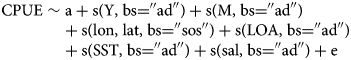
where, a is the intercept, Y is years, M is months, lon is longitude, lat is latitude, LOA is length of overall, SST is sea surface temperature, sal is salinity and s indicates the smoother function of the corresponding independent variable. In the model, bs indicates the (penalized) smoothing basis to use, cs represents the cubic regression spline smooths, sos represents the univariate penalized cubic regression spline smooths. Finally, e is a random error term.
The test of whether the basis dimension for a smooth is adequate (Wood, Reference Wood2017) were done by k-index (the estimate of the residual variance based on differencing residuals) and p-value, computed by simulation. Low p-value may indicate that the basis dimension has been set too low, especially if the reported estimated degrees of freedom (edf) is close to upper limit on the degrees of freedom associated with an s smooth (k'). The procedure automatically selects the degree of smoothing based on the Generalized Cross Validation (GCV) score, which is a proxy for the model predictive performance. However, given the limited number of observations, the model was constrained to be at maximum a quartic relation. Consequently, the maximum degrees of freedom for each smoothing term, indicated by the number of knots (k), were set to 49 for the spatial variable and 39 for the remaining variables (i.e. k = 50 for the spatial variable and k = 40 for the rest of the variables in the GAM formulation). A log link function was assumed, and deficiencies of the fitted model were diagnosed by QQ plot of the deviance residuals and means of randomized quantile residual plots (Foster and Bravington, Reference Foster and Bravington2013; Pedersen et al., Reference Pedersen, Miller, Simpson and Ross2019). Statistical inference was based on the 95% confidence level. The model fitting was accomplished using the ‘mgcv’ library (Wood, Reference Wood2003, Reference Wood2004, Reference Wood2011, Reference Wood2016, Reference Wood2017; Wood et al., Reference Wood, Pya and Säfken2016), and the ‘tidyverse’ (Wickham et al., Reference Wickham, Averick, Bryan, Chang, McGowan, François, Grolemund, Hayes, Henry, Hester, Kuhn, Pedersen, Miller, Bache, Müller, Ooms, Robinson, Seidel, Spinu, Takahashi, Vaughan, Wilke, Woo and Yutani2019), ‘gratia’ (Simpson, Reference Simpson2022), ‘sf’ (Pebesma, Reference Pebesma2018), ‘ggspatial’ (Dunnington, Reference Dunnington2021), ‘scales’ (Wickham and Seidel, Reference Wickham and Seidel2022) and ‘rnaturalearth’ packages (South et al., Reference South, Michael and Massicotte2024) were also required under the R language environment (R Core Team, 2022).
Results
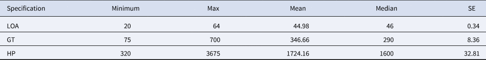
The sampled Turkish ABFT purse seines ranged from 20 to 64 m (average: 44.9 ± 0.4 m) in length (LOA) and 320 to 3675 hp (average: 1724 ± 32.8 hp) in machine power (Table 1).
Table 1. Summary of the sampled fishing vessels
The number of ABFT caught within each operation varied between 1 and 2000. Meanly 99.79 ± 9.57 BFT were caught. During the catching operations the recorded weight of individual ABFT ranged from 8 to 350 kg. A total of 386 CPUE values for ABFT were calculated, which ranged between 0.05 and 60 t ⋅ (haul day)–1 with mean CPUE of 5.51 ± 0.54 t ⋅ (haul day)–1. Moreover, the smallest median was 0.3 t ⋅ (haul day)–1 for July and the maximum median was recorded as 4.8 t ⋅ (haul day)–1 for June (Figure 1). The range of variability around the median value in June was between 2 and 20 t ⋅ (haul day)–1. After 2001, fishing activity shifted to the southern part of Turkey and was mainly performed in May (Figure 2).
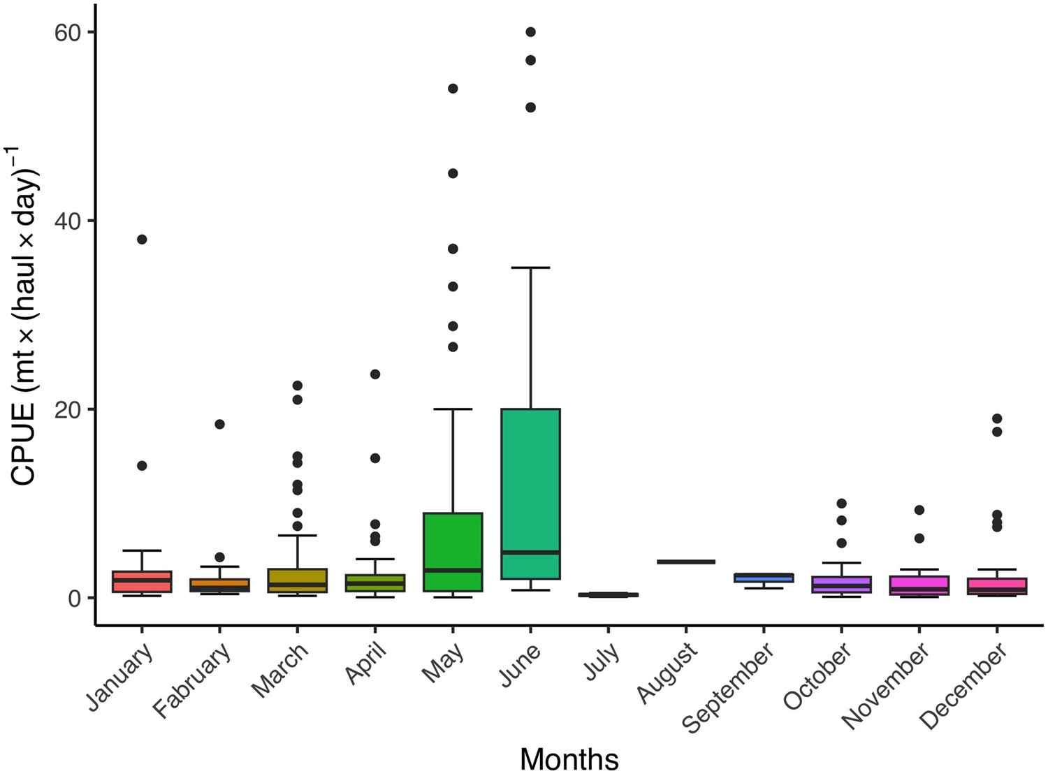
Figure 1. The CPUE values of Turkish ABFT fishery in the eastern Mediterranean by months.
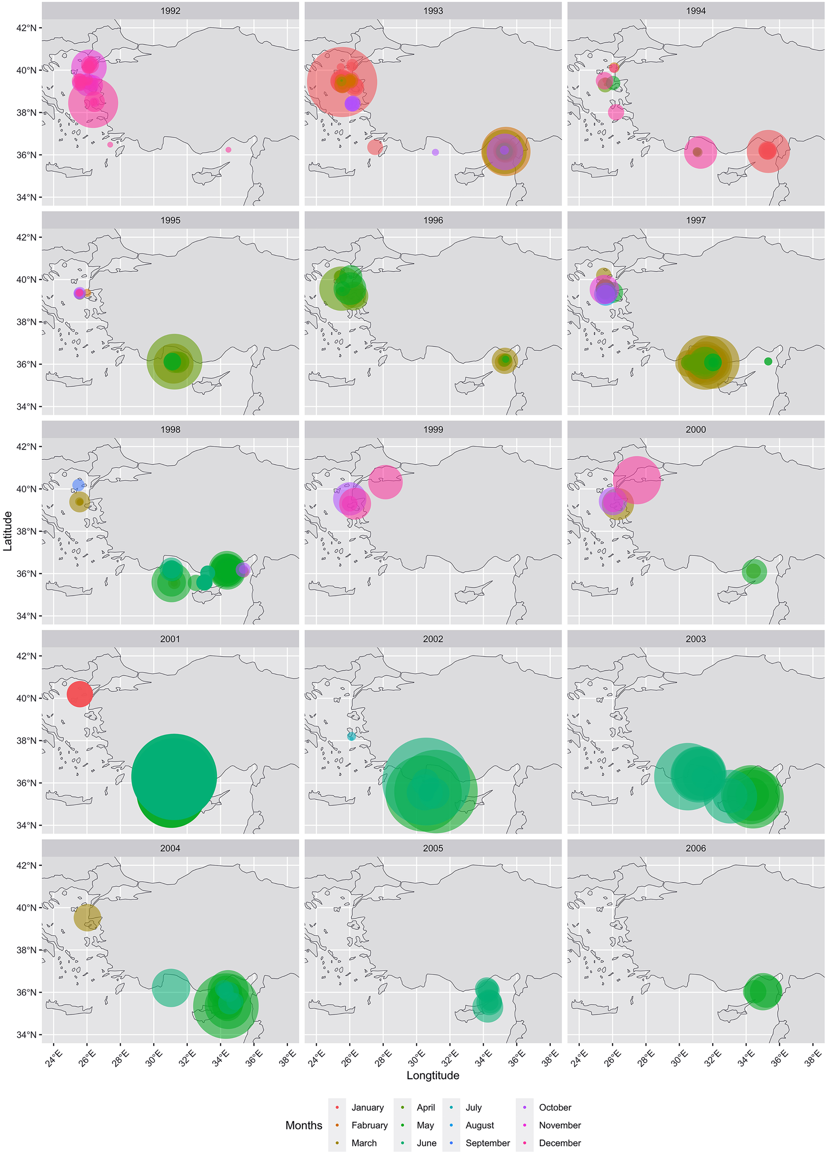
Figure 2. Spatial distribution of the ABFT fishery by year and months.
The diagnostic information regarding the fitting procedure and results indicates that the basis dimensions used for the smooth terms were appropriate (Table 2). Additionally, Figure 3A, which presents the deviance residuals plotted against the approximate theoretical quantiles of the deviance residual distribution, demonstrates that the model's distributional assumptions were mostly satisfied. While there were three values that appeared to be lower and did not fit the model perfectly, we did not consider them as outliers and chose not to remove them. This decision was based on their association with the fishery season during 1992 and 1994, which represents an early period. Furthermore, Figure 3B shows that the response data were independent, and thus the residuals appeared reasonably well-distributed. The proportion of explained deviance was calculated to be 80.2%. Hence, we can confidently argue that the model fit very well, and there were no significant confidence intervals observed.
Table 2. The result of basis dimensions of model
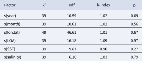
k’ = upper limit on the degrees of freedom associated with an s smooth, edf = estimated degrees of freedom, k-index = ratio of neighbour differencing scale estimate to fitted model scale estimate, p = p-value.
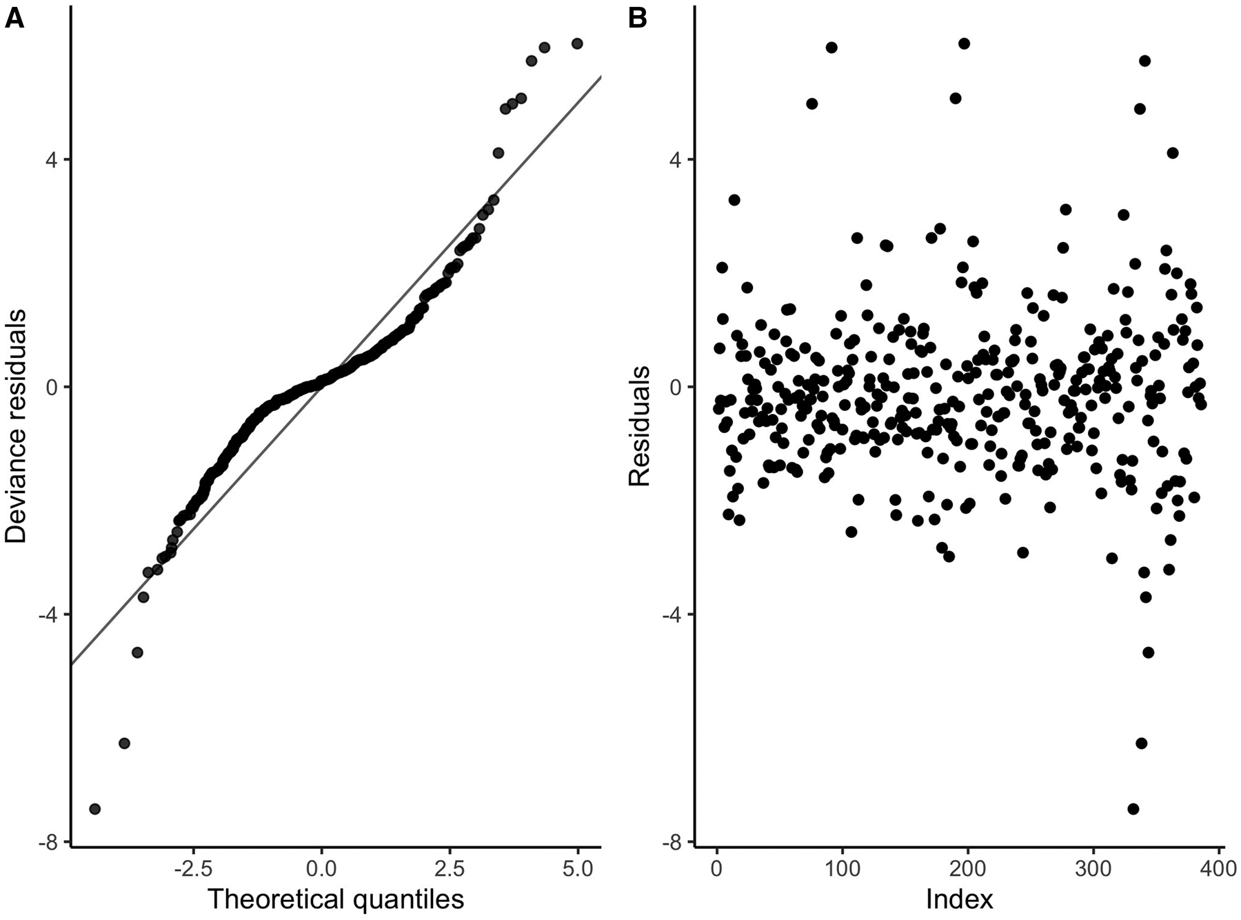
Figure 3. (A) QQ-plot of residuals (black). The grey line indicates the 1–1 line. (B) Means of randomized quantile residuals.
The analysis of the deviance table revealed that all variables, except SST, were found to be significant (Table 3). Furthermore, Figure 4A displayed an undulant pattern in the line. Negative effects were predominantly observed on the CPUE in June and July (Figure 4B). Despite the presence of wide confidence intervals in certain parts of the plots, Figure 4C and 4D depicted relatively stable lines. While a negative effect was evident around 20 °C, the remainder of the line appeared to be stable in Figure 4E. These figures corroborated the findings presented in Table 3. The effect of spatial data on CPUE was greatest along the Turkish coast and eastern Mediterranean (Figure 5). Consequently, the results indicated that the year, month, LOA, salinity and area were significant explanatory factors, whereas SST had little influence on the CPUE.
Table 3. Analysis of deviance table for the GAM model fitted to the CPUE data of the BFT purse seine fleet
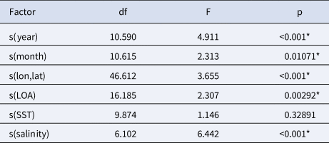
*<0.05; df, degrees of freedom; F, F-value; p, p-value; s(x), smoother function of the corresponding independent variable; lon, longitude; lat, latitude; LOA, length overall; SST, sea surface temperature.
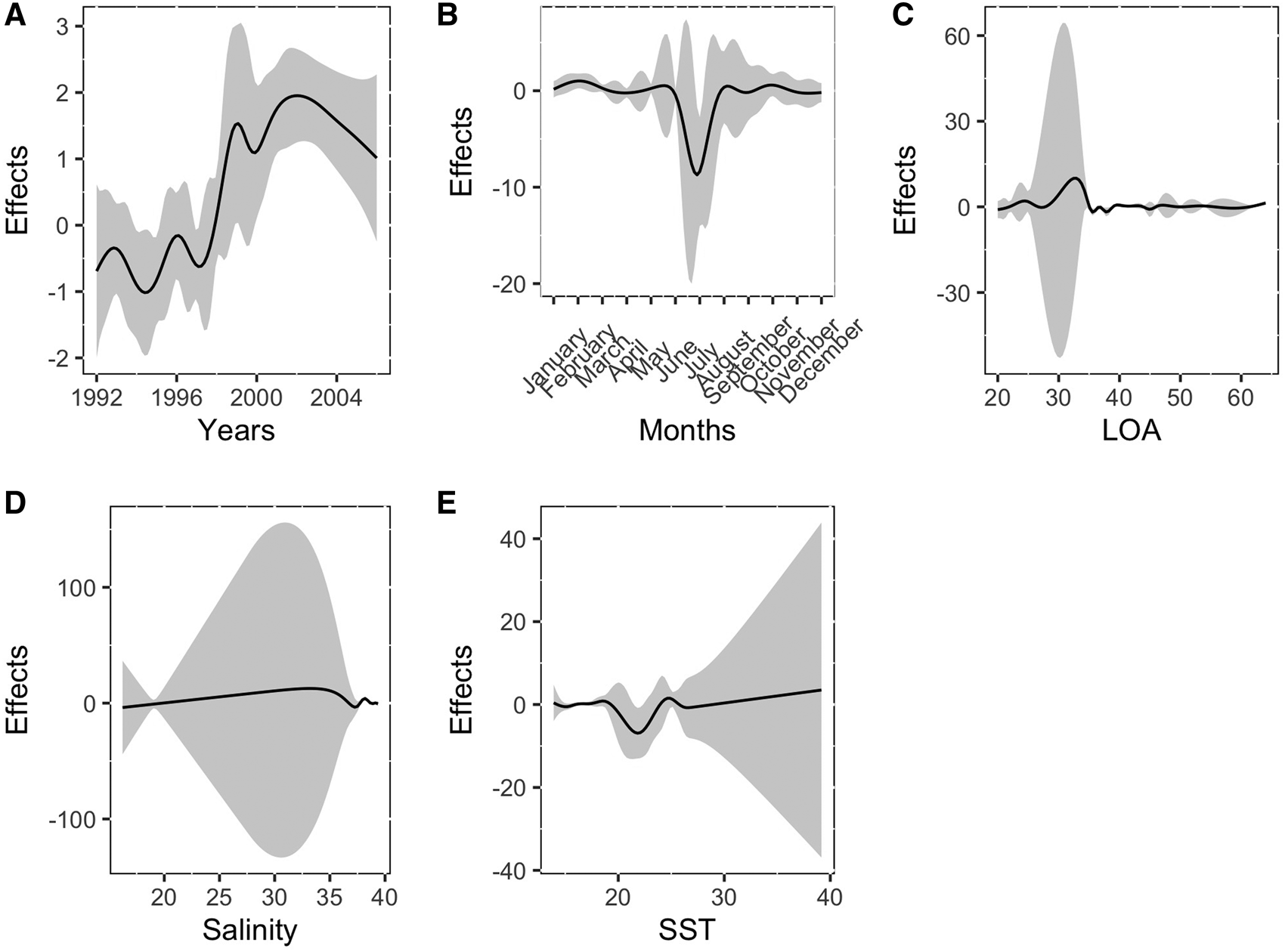
Figure 4. GAM estimated effect of years (A), months (B), LOA (C), salinity (D), SST (E) on CPUE for ABFT PS fishery (grey area corresponds to the 95% confidence intervals of the estimates).
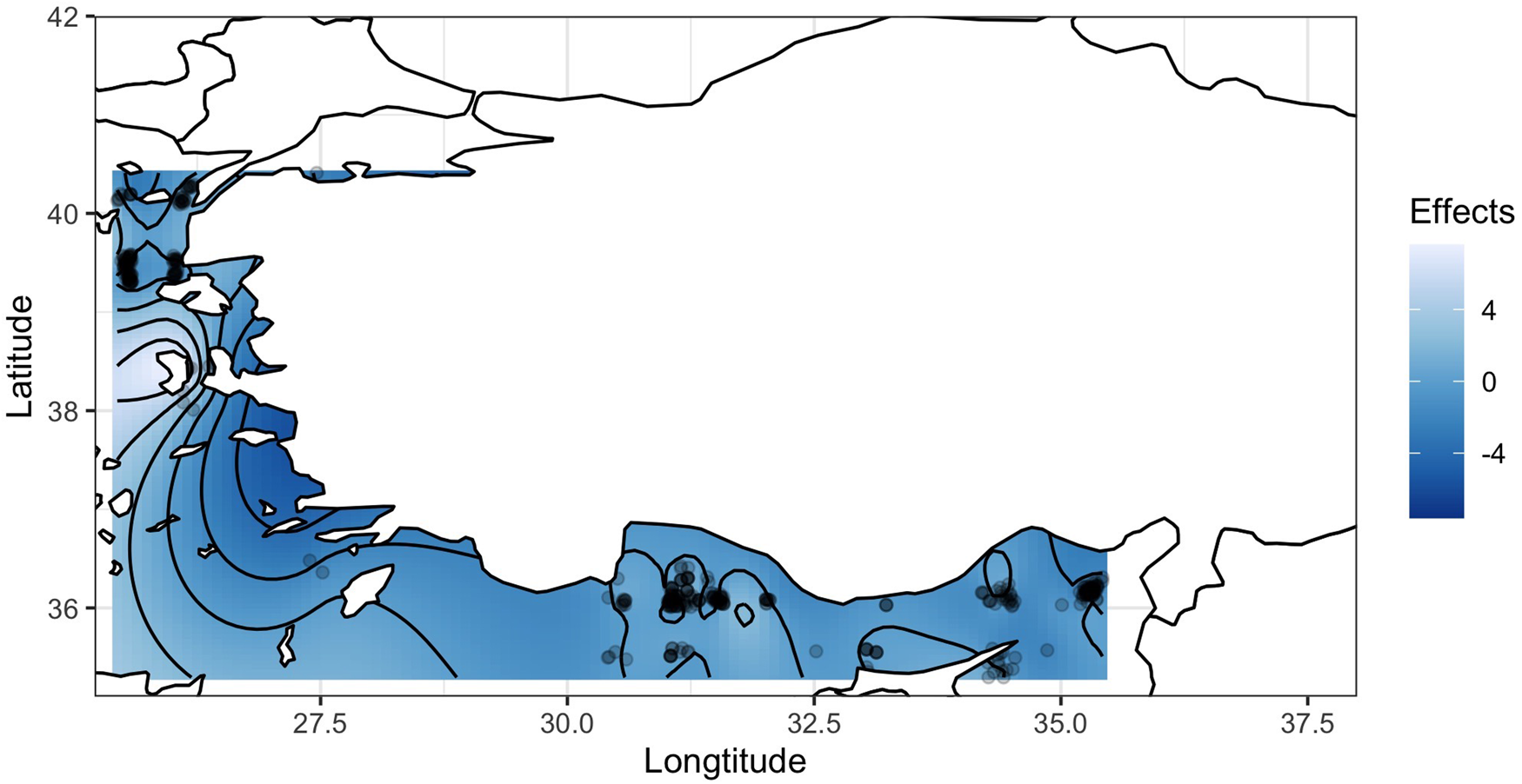
Figure 5. GAM estimated effect of spatial data on CPUE for ABFT PS fishery.
Discussion
Purse seine became the main catching method for ABFT in Turkish fishery since the 1950s. Initially purse seiners mainly targeted the ABFT under the sardine purse seines for feeding or small schools off the coast. Due to the decrease in anchovy fishing in the 1990s, purse seine fishermen started to target tuna and exported it to far Eastern countries (Mert et al., Reference Mert, Oray, Patrona, Karakulak, Kayabaşı, Gündoğdu and Miyake2000). With the start of tuna farms in Turkey in 2003, there have been significant changes in tuna fishing time and areas, and fishermen have targeted more breeding populations (Karakulak et al., Reference Karakulak, Öztürk, Yıldız, Daniel, Gavin and Alejandro2016). In this study the temporal and spatial variations in the tuna fishery between 1992 and 2006 were analysed.
The study presented comprehensive CPUE indices ranging from 0.05 to 60 t ⋅ (haul day)–1, with a mean CPUE of 5.51 ± 0.54 t ⋅ (haul day)–1. In comparison, Zarrad and Missaou (Reference Zarrad and Missaou2018) reported standardized CPUE values of the Tunisian purse seine fleet ranging from 1.4 to 6.6 t ⋅ day–1. The discrepancies in CPUE values can be attributed to the month restrictions imposed in Tunisia. The fishing season was two months until 2009, and since then, it has been reduced to one month. Additionally, Karakulak (Reference Karakulak2004) calculated CPUE values for the Turkish fleet ranging from 3.22 to 7.32 t, with an average of 5.58 t per year. It is notable that CPUE values in Turkey were lower during the 1990s when tuna fishing predominantly occurred in autumn and winter. However, a shift towards fishing in May, particularly during the breeding period, as indicated by Karakulak et al. (Reference Karakulak, Oray, Corriero, Deflorio, Santamaria, Desantis and De Metrio2004) and Corriero et al. (Reference Corriero, Karakulak, Santamaria, Deflorio, Spedicato, Addis, Desantis, Cirillo, Fenech-Farrugia, Vassallo-Agius, Serna, Oray, Cau, Megalofonou and Metrio2005), resulted in a significant increase in CPUE data. Furthermore, Yalçın (Reference Yalçın2022) argued that factors such as shooting duration, closing the lacing duration, current speed at 10 m, setting speed, sinking speed and length-height ratio play crucial roles in the success of ABFT catching by purse seining, in addition to the physical variables of the sea.
The month trend of standardized CPUE showed the slight decrease between July and August in this study. The Eastern ABFT stock spawns from June to July in the Mediterranean Sea then migrates to their feeding areas (Piccinetti and Piccinetti-Manfrin, Reference Piccinetti and Piccinetti-Manfrin1970; Richards, Reference Richards1976; Dicenta and Piccinetti, Reference Dicenta and Piccinetti1978). Some of them move to areas between NW coasts of Africa and Norway and even trans-Atlantic areas (Mather et al., Reference Mather, Mason and Jones1995; Block et al., Reference Block, Dewar, Blackwell, Williams, Prince, Farwell, Boustany, Teo, Seitz, Walli and Fudge2001; Rodríguez-Marín et al., Reference Rodríguez-Marín, Arrizabalaga, Ortiz, Rodríguez-Cabello, Moreno and Kell2003). Temporal distribution of bluefin tuna catches indicated that the higher probability of catching of ABFT is related with the species’ spawning period in the eastern Mediterranean. Furthermore, the fishing grounds in Mediterranean changed from juveniles to spawners and fishing has been performed in spawning areas after 2000s (Gordoa et al., Reference Gordoa, Rouyer and Ortiz2019). As well known, the purse seiners became the main provider of live fish to farms in Mediterranean. Therefore, the fishing strategy for ABFT was only set up to catch larger fish in spawning areas for the Turkish purse seine fleet. This is also the same for other fleets of Mediterranean countries. The tagging studies carried out in the Eastern Mediterranean reported that ABFT do not prefer to migrate through the Gibraltar straight. In contrast, ABFT stay in the Eastern Mediterranean and also move to the Aegean Sea for feeding (de Metrio et al., Reference de Metrio, Oray, Arnold, Lutcavage, Deflorio, Cort, Karakulak, Anbar and Ultanur2004, Reference de Metrio, Arnold, de La Serna, Cort, Block, Megalofonou, Lutcavage, Oray and Deflorio2005). The ABFT catches between October and April during the 1990s also indicate that the Aegean Sea is an important feeding area after ABFT have spawned in the Eastern Mediterranean (Karakulak and Oray, Reference Karakulak and Oray1995; Oray and Karakulak, Reference Oray and Karakulak1997; Druon et al., Reference Druon, Fromentin, Hanke, Arrizabalaga, Damalas, Tičina, Quílez-Badia, Ramirez, Arregui, Tserpes, Reglero, Deflorio, Oray, Saadet Karakulak, Megalofonou, Ceyhan, Grubišić, MacKenzie, Lamkin, Afonso and Addis2016).
In this study, we only put one fishing vessel measurement (LOA) into the model to avoid the unstable model-fitting process and overfitting. Inclusion of all quantities of fishing vessel as explanatory variables would not improve the predictive ability of the model (Maunder and Punt, Reference Maunder and Punt2004). However, the standardization procedure showed that length of fishing vessel has a relatively minor explanatory effect on the CPUE in the purse seine fishery. Moreover, Rodríguez-Marín et al. (Reference Rodríguez-Marín, Arrizabalaga, Ortiz, Rodríguez-Cabello, Moreno and Kell2003) stated that the results related with vessel size should be interpreted with caution, because there are several possible underlying effects such as technological improvements in fishing gear, electronics and fishing power. We believe that tuna purse seiners had become more accustomed to the new technology, and more efficient at identifying large schools of ABFT, year by year.
With respect to spatial interaction effects, the area around Antalya Bay had higher value than the area around Gokceada Island. These two areas are quite different in terms of fishing strategy and fishing season. Furthermore, there was an area of positive value near shore along Turkey. These results indicate area effects on CPUE vary according to area. We also found the high effect on coastal areas. Damalas and Megalofonou (Reference Damalas and Megalofonou2012) explained the same situation with the reflecting foraging of ABFT, as prey usually congregate near land or on seamounts and banks. Moreover, the thermocline is a key factor in depth distribution of tunas (Abascal et al., Reference Abascal, Peatman, Leroy, Nicol, Schaefer, Fuller and Hampton2018). Actually, the distribution of ABFT has been affecting from many biotic and abiotic environmental variables such as SST, salinity, chlorophyll-a, etc. We found that the salinity was a significant explanatory factor, whereas SST had little influence on the CPUE in this study. Arrizabalaga et al. (Reference Arrizabalaga, Dufour, Kell, Merino, Ibaibarriaga, Chust, Irigoien, Santiago, Murua, Fraile, Chifflet, Goikoetxea, Sagarminaga, Aumont, Bopp, Herrera, Marc Fromentin and Bonhomeau2015) reported that ABFT does not exhibit a well-established temperature preference but rather demonstrates a wide temperature tolerance range (approximately between 1 and 20 °C). On the other hand, salinity can have a notable impact on the large-scale spatial distribution of ABFT (Reygondeau et al., Reference Reygondeau, Maury, Beaugrand, Fromentin, Fonteneau and Cury2012; Fromentin et al., Reference Fromentin, Reygondeau, Bonhommeau and Beaugrand2014). Additionally, Teo and Block (Reference Teo and Block2010) stated that ABFT CPUE increased substantially during the breeding months in areas with negative sea surface height anomalies and cooler SSTs. We believe that the reason SST did not significantly affect CPUE in our study could be attributed to the development of tuna fattening in Turkey and the fact that fishing is limited to a specific area during the breeding period.
Akyüz and Artüz (Reference Akyüz and Artüz1957) documented the length distribution of ABFT caught in the Bosphorus and Marmara Sea from 1955 to 1956, which ranged from 120 to 330 cm, with an average length of 228.9 ± 2.8 cm. On the other hand, Karakulak and Oray (Reference Karakulak and Oray1995) reported the size distribution of tuna caught in the Aegean Sea during the 1990s, ranging from 50 to 240 cm, and in the Levantine Sea, it ranged from 120 to 230 cm.
Since the initiation of tuna farming activities, the predominant method of capturing tuna in Turkish waters has been through cage farming. In accordance with the ICCAT recommendation (Rec. 19-04), the use of stereo-camera technology has become obligatory for estimating the number, weight and size/age distribution of the captured fish. Ortiz et al. (Reference Ortiz, Karakulak, Mayor and Paga2021) conducted a study examining data obtained from both farms and camera images, revealing a significant shift in the size distribution of fish caught by the Turkish tuna purse seine flotilla. While larger fish (>200 cm SFL) were once abundant in previous years, since 2017, medium-sized tuna (120–140 cm SFL) have become more prevalent, resulting in a notable increase in catch. The proportion of medium-sized fish now accounts for 60% by weight (80% numerically), while the proportion of large fish stands at 5%. Evaluation of fishing activities uncovered a doubling in the number of fishing boats and a fivefold increase in the number of fishing operations. Several factors contribute to this shift, including rising water temperatures in the Levantine Sea, where fishing is intense, the proliferation of Lessepsian species, ongoing gas/oil exploration studies in the Eastern Mediterranean and the overall increase in fishing activities. Further investigation is required to understand the underlying reasons for the decline in the population of larger fish.
In this paper, we utilized a generalized additive model to standardize the CPUE of ABFT in the Eastern Mediterranean purse seine fishery, incorporating spatial data as a variable. Given the economic importance and stock status of ABFT, there is a pressing need for a better understanding of its habitat and spatial dynamics. We strongly believe that considering the spatial dynamics of ABFT is crucial if we aim to mitigate the impact of fisheries on the ecosystem and implement effective remedies.
Data availability
The data that support the findings of this study are available from the corresponding author, upon reasonable request.
Author contributions
F.S. Karakulak: collecting data, conceptualization and editing. T. Ceyhan: writing the draft text, modelling, conceptualization, review and editing processes.
Financial support
There was no external financial support provided for the research conducted in the preparation of this manuscript.
Competing interests
None.
Ethical standards
Not applicable.


 Open access