


1. Introduction
1·1. Background
It is a simple consequence of the Lebesgue density theorem that subsets of
 $\mathbb{R}^n$
of positive Lebesgue measure contain a translated and scaled copy of every finite point set for an interval worth of scalings [
Reference Steinhaus24
]. Under more general assumptions on E, a problem of great current interest is that of describing the set of configurations that exists within E. This includes finding conditions on the structure or size of E that guarantee the existence of various patterns within E, see, for instance, [
Reference Bourgain2, Reference Chan, Łaba and Pramanik4, Reference Falconer and Yavicoli6, Reference Furstenberg, Katznelson and Weiss8, Reference Iosevich and Liu15, Reference Iosevich and Magyar16, Reference Ziegler28
], as well as the more quantitative question of describing the size of the set of similar copies of a given configuration [
Reference Falconer and Yavicoli6, Reference Grafakos, Greenleaf, Iosevich and Palsson10–Reference Greenleaf, Iosevich and Taylor13, Reference McDonald18, Reference Yavicoli27
]. We focus on the latter question. A particularly simple object of study is the set of chains of distances determined by a set E:
$\mathbb{R}^n$
of positive Lebesgue measure contain a translated and scaled copy of every finite point set for an interval worth of scalings [
Reference Steinhaus24
]. Under more general assumptions on E, a problem of great current interest is that of describing the set of configurations that exists within E. This includes finding conditions on the structure or size of E that guarantee the existence of various patterns within E, see, for instance, [
Reference Bourgain2, Reference Chan, Łaba and Pramanik4, Reference Falconer and Yavicoli6, Reference Furstenberg, Katznelson and Weiss8, Reference Iosevich and Liu15, Reference Iosevich and Magyar16, Reference Ziegler28
], as well as the more quantitative question of describing the size of the set of similar copies of a given configuration [
Reference Falconer and Yavicoli6, Reference Grafakos, Greenleaf, Iosevich and Palsson10–Reference Greenleaf, Iosevich and Taylor13, Reference McDonald18, Reference Yavicoli27
]. We focus on the latter question. A particularly simple object of study is the set of chains of distances determined by a set E:
 \begin{equation}\left\{\left(|x^1-x^2|,\dots,|x^k-x^{k+1}|\right)\in \mathbb{R}^k\,{:}\,x^i\in E \text{ distinct}\right\}.\end{equation}
Such objects are studied by Bennett, Iosevich, and the second listed author in [
Reference Bennett, Iosevich and Taylor1
]. They prove that if the Hausdorff dimension of E is greater than
 $({d+1})/{2}$
, the above set has non-empty interior in
$({d+1})/{2}$
, the above set has non-empty interior in
 $\mathbb{R}^k$
. In the plane, it was shown by Ou and the second author [
Reference Ou and Taylor21
] that the set of distance chains has positive Lebesgue measure when
$\mathbb{R}^k$
. In the plane, it was shown by Ou and the second author [
Reference Ou and Taylor21
] that the set of distance chains has positive Lebesgue measure when
 $\dim_H\!(E)>5/4$
. However, when
$\dim_H\!(E)>5/4$
. However, when
 $\dim_H\!(E)<3/2$
it is not known whether the set of distance chains has non-empty interior.
$\dim_H\!(E)<3/2$
it is not known whether the set of distance chains has non-empty interior.
The aim of this paper is to study the interior of sets of distance chains (and more generally distance trees) in subsets of
 $\mathbb{R}^2$
under structural assumptions different from having large Hausdorff dimension. We will consider plane sets of the form
$\mathbb{R}^2$
under structural assumptions different from having large Hausdorff dimension. We will consider plane sets of the form
 $K_1\times K_2$
, where each
$K_1\times K_2$
, where each
 $K_j$
is a sufficiently “thick” Cantor set. The precise definition of thickness is due to Newhouse ([
Reference Newhouse20
], also see [
Reference Palis and Takens22
] and [
Reference Yavicoli26
]) and is given below (Definition 1·2), but can be intuitively described as follows. Suppose we construct a Cantor set in countably many stages by taking
$K_j$
is a sufficiently “thick” Cantor set. The precise definition of thickness is due to Newhouse ([
Reference Newhouse20
], also see [
Reference Palis and Takens22
] and [
Reference Yavicoli26
]) and is given below (Definition 1·2), but can be intuitively described as follows. Suppose we construct a Cantor set in countably many stages by taking
 $K_0=[0,1]$
,
$K_0=[0,1]$
,
 $K_1=[0,a]\cap [b,1]$
, and so on, so that
$K_1=[0,a]\cap [b,1]$
, and so on, so that
 $K_n$
is a union of finitely many closed intervals and
$K_n$
is a union of finitely many closed intervals and
 $K_{n+1}$
is obtained from
$K_{n+1}$
is obtained from
 $K_n$
by removing an interior open interval from each. When we consider the sequence of bounded gaps in order of decreasing length, the thickness measures the size of the open intervals being removed, relative to the closed intervals which remain.
$K_n$
by removing an interior open interval from each. When we consider the sequence of bounded gaps in order of decreasing length, the thickness measures the size of the open intervals being removed, relative to the closed intervals which remain.
1·2. Definitions and notation
Definition 1·1 (Cantor sets). A Cantor set is a non-empty subset of
 $\mathbb{R}^d$
which is compact, perfect, and totally disconnected.
$\mathbb{R}^d$
which is compact, perfect, and totally disconnected.
When
 $K\subset \mathbb{R}$
is a Cantor set, we have the following notion of structure.
$K\subset \mathbb{R}$
is a Cantor set, we have the following notion of structure.
Definition 1·2 (Thickness). A gap of a Cantor set
 $K\subset \mathbb{R}$
is a connected component of the complement
$K\subset \mathbb{R}$
is a connected component of the complement
 $\mathbb{R}\setminus K$
. If u is the right endpoint of a bounded gap G, for
$\mathbb{R}\setminus K$
. If u is the right endpoint of a bounded gap G, for
 $b\in \mathbb{R}\cup \{\infty\}$
, let (a, b) be the closest gap to G with the property that
$b\in \mathbb{R}\cup \{\infty\}$
, let (a, b) be the closest gap to G with the property that
 $u<a$
and
$u<a$
and
 $|G|\le b-a$
. The interval (u, a) is called the bridge at u and is denoted B(u). Analogous definitions are made when u is a left endpoint. The thickness of K at u is the quantity
$|G|\le b-a$
. The interval (u, a) is called the bridge at u and is denoted B(u). Analogous definitions are made when u is a left endpoint. The thickness of K at u is the quantity
 \begin{align*}\tau(K,u)\,{:\!=}\,\frac{|B(u)|}{|G|}.\end{align*}
Finally, the thickness of the Cantor set K is the quantity
 \begin{align*}\tau(K)\,{:\!=}\,\inf_u \tau(K,u),\end{align*}
the infimum being taken over all gap endpoints u.
Before moving on, we comment on the relationship between thickness and Hausdorff dimension. One can easily construct a Cantor set K with arbitrarily small thickness and Hausdorff dimension arbitrarily close to 1. This is due to the fact that thickness is defined using an infimum, so one can construct a thin Cantor set by simply ensuring one bridge is much smaller than the corresponding gap. More precisely, for any
 $\delta>0$
and
$\delta>0$
and
 $1< N< \delta^{-1}$
we can construct K as a subset of
$1< N< \delta^{-1}$
we can construct K as a subset of
 $[0,\delta]\cup[N\delta,1]$
. It is clear that Cantor sets of this form can attain any Hausdorff dimension in [0, 1]. Considering the gap
$[0,\delta]\cup[N\delta,1]$
. It is clear that Cantor sets of this form can attain any Hausdorff dimension in [0, 1]. Considering the gap
 $(\delta, N\delta)$
and corresponding bridge
$(\delta, N\delta)$
and corresponding bridge
 $[0,\delta]$
, we conclude that
$[0,\delta]$
, we conclude that
 $\tau(K)\leq {1}/({N-1})$
.
$\tau(K)\leq {1}/({N-1})$
.
On the other hand, large thickness implies large Hausdorff dimension. Specifically, one can prove the bound (see [ Reference Palis and Takens22 , page 77]):
 \begin{equation}\dim_{\rm H}\!(K) \geq \frac{\log{2}}{\log\!{\left( 2 + \frac{1}{\tau(K)} \right) }}.\end{equation}
The study of chains of distances is motivated by the Falconer distance problem, which asks how large the Hausdorff dimension of a set must be to ensure positive measure worth of distances; This amounts to the case
 $k=1$
in the chain problem. For more on the Falconer distance problem, see [
Reference Falconer7, Reference Guth, Iosevich, Ou and Wang14
]. To pose questions about more complex patterns, the language of graph theory is useful. We pause to state some basic definitions.
$k=1$
in the chain problem. For more on the Falconer distance problem, see [
Reference Falconer7, Reference Guth, Iosevich, Ou and Wang14
]. To pose questions about more complex patterns, the language of graph theory is useful. We pause to state some basic definitions.
Definition 1·3 (Graphs). A (finite) graph is a pair
 $G=(V,\mathcal{E})$
, where V is a (finite) set and
$G=(V,\mathcal{E})$
, where V is a (finite) set and
 $\mathcal{E}$
is a set of 2-element subsets of V. If
$\mathcal{E}$
is a set of 2-element subsets of V. If
 $\{i,j\}\in \mathcal{E}$
we say i and j are adjacent and write
$\{i,j\}\in \mathcal{E}$
we say i and j are adjacent and write
 $i\sim j$
.
$i\sim j$
.
Consider a graph with vertex set
 $\{1,\dots,k+1\}$
and edges
$\{1,\dots,k+1\}$
and edges
 $i\sim j$
if and only if
$i\sim j$
if and only if
 $|i-j|=1$
; Such a graph is called a k-chain. Given points
$|i-j|=1$
; Such a graph is called a k-chain. Given points
 $x^1,\dots x^{k+1}$
in the plane, the vector
$x^1,\dots x^{k+1}$
in the plane, the vector
 $(|x^1-x^2|,\dots,|x^k-x^{k+1}|)\in \mathbb{R}^k$
encodes all pairwise distances
$(|x^1-x^2|,\dots,|x^k-x^{k+1}|)\in \mathbb{R}^k$
encodes all pairwise distances
 $|x^i-x^j|$
for which
$|x^i-x^j|$
for which
 $i\sim j$
. The set (1·1) contains all such distance vectors obtained from points in the chosen subset E. This motivates the following general definition.
$i\sim j$
. The set (1·1) contains all such distance vectors obtained from points in the chosen subset E. This motivates the following general definition.
Definition 1·4 (G-distance sets). Let G be a graph on the vertex set
 $\{1,\dots,k+1\}$
with m edges, and let
$\{1,\dots,k+1\}$
with m edges, and let
 $\sim$
denote the adjacency relation on G. Define the G-distance set of E to be
$\sim$
denote the adjacency relation on G. Define the G-distance set of E to be
 \begin{align*}\Delta_G(E)=\left\{\left(|x^i-x^j|\right)_{i\sim j}\,{:}\,x^1,...,x^{k+1}\in E, x^i\neq x^j\right\},\end{align*}
where
 $(|x^i - x^j|)_{i\sim j}$
denotes a vector in
$(|x^i - x^j|)_{i\sim j}$
denotes a vector in
 $\mathbb{R}^m$
with coordinates indexed by the edges of G.
$\mathbb{R}^m$
with coordinates indexed by the edges of G.
The feature of chains that allows us to obtain results is that they can be deconstructed one vertex at a time. Given a k-chain, we may remove the last vertex and its corresponding edge and obtain a
 $(k-1)$
-chain. This allows us to make inductive arguments, reducing results about long chains to results about short chains, and ultimately to results about chains with only one link. This feature is also present in a more general class of graphs, which we define here.
$(k-1)$
-chain. This allows us to make inductive arguments, reducing results about long chains to results about short chains, and ultimately to results about chains with only one link. This feature is also present in a more general class of graphs, which we define here.
Definition 1·5 (Trees). A tree is a connected, acyclic graph; equivalently, a tree is a graph in which any two vertices are connected by exactly one path. If T is a tree, the leaves of T are the vertices which are adjacent to exactly one other vertex of T.
In particular, a k-chain is a tree. The structural property of trees which enables our induction argument is recorded below as a proposition.
Proposition 1·6 (Tree structure). If T is a tree with
 $k+1$
vertices, then T has k edges. Moreover, there is a sequence of trees
$k+1$
vertices, then T has k edges. Moreover, there is a sequence of trees
 $T_1, \dots,T_{k+1}$
such that
$T_1, \dots,T_{k+1}$
such that
 $T_1=T$
and each
$T_1=T$
and each
 $T_{i+1}$
is obtained from
$T_{i+1}$
is obtained from
 $T_i$
by removing one leaf and its corresponding edge.
$T_i$
by removing one leaf and its corresponding edge.
1·3. Main results
Our first result builds on the work in [
Reference Simon and Taylor23
] of Simon and the second listed author, where it is shown
 $\Delta_x(K\times K) = \{|x-y|\,{:}\, y \in K\times K\}$
has non-empty interior for each
$\Delta_x(K\times K) = \{|x-y|\,{:}\, y \in K\times K\}$
has non-empty interior for each
 $x\in \mathbb{R}^2$
provided that
$x\in \mathbb{R}^2$
provided that
 $K\subset \mathbb{R}$
is a Cantor set satisfying
$K\subset \mathbb{R}$
is a Cantor set satisfying
 $\tau(K)> 1$
.
$\tau(K)> 1$
.
Theorem 1·7 (Interior of tree distance sets). Let
 $K_1,K_2$
be Cantor sets satisfying
$K_1,K_2$
be Cantor sets satisfying
 $\tau(K_1)\cdot \tau(K_2) > 1$
For any finite tree T, the set
$\tau(K_1)\cdot \tau(K_2) > 1$
For any finite tree T, the set
 $\Delta_T(K_1\times K_2)$
has non-empty interior.
$\Delta_T(K_1\times K_2)$
has non-empty interior.
Theorem 1·7 also holds if the Euclidean norm is replaced with more general norms; see Theorem 1·14 below. Recall that if
 $E\subset \mathbb{R}^2$
and
$E\subset \mathbb{R}^2$
and
 $\dim_{\rm H}\!(E)>{5}/{4}$
, then
$\dim_{\rm H}\!(E)>{5}/{4}$
, then
 $\Delta_T(E)$
has positive Lebesgue measure. However, when
$\Delta_T(E)$
has positive Lebesgue measure. However, when
 $\dim_H\!(E)<{3}/{2}$
it is not known whether
$\dim_H\!(E)<{3}/{2}$
it is not known whether
 $\Delta_T(E)$
has non-empty interior. In light of (1·2), if
$\Delta_T(E)$
has non-empty interior. In light of (1·2), if
 $\tau(K_j)>1$
then
$\tau(K_j)>1$
then
 $\dim_{\rm H}\!(K_1\times K_2)> {2\cdot\log 2}/{\log 3}\approx 1.26$
. Therefore, based solely on dimension we can conclude
$\dim_{\rm H}\!(K_1\times K_2)> {2\cdot\log 2}/{\log 3}\approx 1.26$
. Therefore, based solely on dimension we can conclude
 $\Delta_T(K_1\times K_2)$
has positive Lebesgue measure, but not necessarily non-empty interior.
$\Delta_T(K_1\times K_2)$
has positive Lebesgue measure, but not necessarily non-empty interior.
Beyond trees, the existence of patterns in thick subsets of
 $\mathbb{R}^d$
with rigid structure was investigated in [
Reference Yavicoli25
] when
$\mathbb{R}^d$
with rigid structure was investigated in [
Reference Yavicoli25
] when
 $d=1$
, and in [
Reference Falconer and Yavicoli6, Reference Yavicoli27
] when
$d=1$
, and in [
Reference Falconer and Yavicoli6, Reference Yavicoli27
] when
 $d\geq 1$
. In [
Reference Yavicoli25
], it is shown that, given any compact set C in
$d\geq 1$
. In [
Reference Yavicoli25
], it is shown that, given any compact set C in
 $\mathbb{R}$
with thickness
$\mathbb{R}$
with thickness
 $\tau$
, there is an explicit number
$\tau$
, there is an explicit number
 $N(\tau)$
such that C contains a translate of all sufficiently small similar copies of every finite set in
$N(\tau)$
such that C contains a translate of all sufficiently small similar copies of every finite set in
 $\mathbb{R}$
with at most
$\mathbb{R}$
with at most
 $N(\tau)$
elements. Higher dimensional analogues of these results are subsequently given in [
Reference Falconer and Yavicoli6
]. The only drawback is that the theorems in [
Reference Falconer and Yavicoli6, Reference Yavicoli25
] assume very large thickness; moreover, the threshold depends on the size of the configuration one wants to find. For instance, in order to ensure
$N(\tau)$
elements. Higher dimensional analogues of these results are subsequently given in [
Reference Falconer and Yavicoli6
]. The only drawback is that the theorems in [
Reference Falconer and Yavicoli6, Reference Yavicoli25
] assume very large thickness; moreover, the threshold depends on the size of the configuration one wants to find. For instance, in order to ensure
 $N(\tau)\geq 3$
, one needs
$N(\tau)\geq 3$
, one needs
 $\tau$
at least on the order of
$\tau$
at least on the order of
 $10^9$
. In contrast, our results for trees apply to any Cantor sets of thickness greater than 1, regardless of how large the tree is.
$10^9$
. In contrast, our results for trees apply to any Cantor sets of thickness greater than 1, regardless of how large the tree is.
Another Falconer type problem which has received much attention is obtained by replacing the Euclidean distance with other geometric quantities, notably dot products. We make the following definition.
Definition 1·8 (Dot product sets). Given
 $E\subset\mathbb{R}^d$
, the dot product set of E is the set
$E\subset\mathbb{R}^d$
, the dot product set of E is the set
 \begin{align*}\Pi(E)=\{x\cdot y\,{:}\, x,y\in E\}.\end{align*}
We also consider the pinned dot product set
 \begin{align*}\Pi_x(E)=\{x\cdot y\,{:}\,y\in E\}.\end{align*}
Finally, given a graph G on vertices
 $\{1,...,k+1\}$
, define
$\{1,...,k+1\}$
, define
 \begin{align*}\Pi_{G}(E)=\{(x^i\cdot x^j)_{i\sim j}\,{:}\,x^1,...,x^{k+1}\in E\}.\end{align*}
When
 $E\subset \mathbb{R}^d$
is a set of sufficient Hausdorff dimension, the dot product set is treated in [
Reference Eswarathasan, Iosevich and Taylor5
, theorem 1·8]. In particular, it is shown there that if
$E\subset \mathbb{R}^d$
is a set of sufficient Hausdorff dimension, the dot product set is treated in [
Reference Eswarathasan, Iosevich and Taylor5
, theorem 1·8]. In particular, it is shown there that if
 $\dim_{\rm H}\!(E) >({d+1})/{2}$
, then
$\dim_{\rm H}\!(E) >({d+1})/{2}$
, then
 $\Pi(E)$
has positive measure. The related set
$\Pi(E)$
has positive measure. The related set
 $\{x^\perp\cdot y\,{:}\,x,y\in E\}$
, where
$\{x^\perp\cdot y\,{:}\,x,y\in E\}$
, where
 $x^\perp=(\!-x_2,x_1)$
when
$x^\perp=(\!-x_2,x_1)$
when
 $d=2$
, is the set of (signed) areas of parallelograms spanned by points of E. Similar to the above definition, for any graph G one can consider the vector which encodes all areas determined by points
$d=2$
, is the set of (signed) areas of parallelograms spanned by points of E. Similar to the above definition, for any graph G one can consider the vector which encodes all areas determined by points
 $x^i,x^j$
such that
$x^i,x^j$
such that
 $i\sim j$
. This problem was investigated by the first author in [
Reference McDonald18
] in the case where G is a complete graph, and the analogous problem in higher dimensions was studied by the first author and Galo in [
Reference Galo and McDonald9
].
$i\sim j$
. This problem was investigated by the first author in [
Reference McDonald18
] in the case where G is a complete graph, and the analogous problem in higher dimensions was studied by the first author and Galo in [
Reference Galo and McDonald9
].
In the setting where one is considering sets E with large Hausdorff dimension, the proofs of distance and dot product results are generally similar in complexity. However, in the setting where
 $E= K\times K$
, where K is a sufficiently thick Cantor set, the dot product problem is considerably more straightforward than to the distance problem. We nevertheless record the result here and provide its proof in Section 3 as a demonstration of how our techniques vary in these two regimes.
$E= K\times K$
, where K is a sufficiently thick Cantor set, the dot product problem is considerably more straightforward than to the distance problem. We nevertheless record the result here and provide its proof in Section 3 as a demonstration of how our techniques vary in these two regimes.
Theorem 1·9 (Interior of tree dot product sets). Let K be a Cantor set satisfying
 $\tau(K)\geq 1$
. For any finite tree T, the set
$\tau(K)\geq 1$
. For any finite tree T, the set
 $\Pi_{T}(K\times K)$
has non-empty interior.
$\Pi_{T}(K\times K)$
has non-empty interior.
Our next main theorem concerns the standard middle thirds Cantor set, which we will denote
 $C_{1/3}$
throughout this paper. Note that Theorem 1·7 does not apply to
$C_{1/3}$
throughout this paper. Note that Theorem 1·7 does not apply to
 $C_{1/3}$
, as the hypothesis of that theorem is
$C_{1/3}$
, as the hypothesis of that theorem is
 $\tau(K)>1$
and clearly
$\tau(K)>1$
and clearly
 $\tau(C_{1/3})=1$
. While we do not expect that Theorem 1·7 can be extended to the
$\tau(C_{1/3})=1$
. While we do not expect that Theorem 1·7 can be extended to the
 $\tau(K)=1$
case in general, this weaker thickness condition together with the self similarity of
$\tau(K)=1$
case in general, this weaker thickness condition together with the self similarity of
 $C_{1/3}$
allow us to modify the proof in that case. The result is as follows.
$C_{1/3}$
allow us to modify the proof in that case. The result is as follows.
Theorem 1·10 (Interior of T distance sets in the middle third Cantor set). For any finite tree T, the set
 $\Delta_{T}(C_{1/3}\times C_{1/3})$
has non-empty interior.
$\Delta_{T}(C_{1/3}\times C_{1/3})$
has non-empty interior.
Having established results for the Euclidean distance and dot products, we turn to the more general setting of
 $(G,\phi)$
distance trees.
$(G,\phi)$
distance trees.
Definition 1·11 (
 $ (G,\phi)$
distance sets). Let G be a graph on the vertex set
$ (G,\phi)$
distance sets). Let G be a graph on the vertex set
 $\{1,\dots,k+1\}$
with m edges, and let
$\{1,\dots,k+1\}$
with m edges, and let
 $\sim$
denote the adjacency relation on G. Given a function
$\sim$
denote the adjacency relation on G. Given a function
 $\phi\,{:}\,\mathbb{R}^d\times \mathbb{R}^d\rightarrow \mathbb{R}$
, define the
$\phi\,{:}\,\mathbb{R}^d\times \mathbb{R}^d\rightarrow \mathbb{R}$
, define the
 $(G,\phi)$
-distance set of E to be
$(G,\phi)$
-distance set of E to be
 \begin{align*}\Delta_{(G, \phi)}(E)=\{ (\phi( x^i,x^j))_{i\sim j}\,{:}\,x^1,...,x^{k+1}\in E, x^i\neq x^j\}.\end{align*}
We require the following derivative condition on
 $\phi$
.
$\phi$
.
Definition 1·12 (Derivative condition). Let
 $\phi\,{:}\, \mathbb{R}^2 \times \mathbb{R}^2\rightarrow \mathbb{R}$
be a
$\phi\,{:}\, \mathbb{R}^2 \times \mathbb{R}^2\rightarrow \mathbb{R}$
be a
 $C^1$
function on
$C^1$
function on
 $A\times B$
, for open sets
$A\times B$
, for open sets
 $A, B\subset \mathbb{R}^2$
. We say that
$A, B\subset \mathbb{R}^2$
. We say that
 $\phi$
satisfies the derivative condition on
$\phi$
satisfies the derivative condition on
 $A\times B$
if for each
$A\times B$
if for each
 $x\in A$
, if
$x\in A$
, if
 $\varphi_x(y)= \phi(x,y)$
, then the partial derivatives of
$\varphi_x(y)= \phi(x,y)$
, then the partial derivatives of
 $\varphi$
are bounded away from zero on B.
$\varphi$
are bounded away from zero on B.
Note 1·13. Note that the derivative condition is satisfied, for instance, by
 $\phi(x,y) = |x-y|_p$
, the p-norm, whenever
$\phi(x,y) = |x-y|_p$
, the p-norm, whenever
 $p\geq1$
, and
$p\geq1$
, and
 $\phi(x,y) = x\cdot y $
for appropriate choices of A and B.
$\phi(x,y) = x\cdot y $
for appropriate choices of A and B.
Theorem 1·14 (Interior of
 $ (T,\phi)$
distance sets). Let
$ (T,\phi)$
distance sets). Let
 $K_1,K_2\subset \mathbb{R}$
be Cantor sets satisfying
$K_1,K_2\subset \mathbb{R}$
be Cantor sets satisfying
 $\tau(K_1)\cdot \tau(K_2) > 1$
. Suppose
$\tau(K_1)\cdot \tau(K_2) > 1$
. Suppose
 $\phi\,{:}\, \mathbb{R}^2 \times \mathbb{R}^2\rightarrow \mathbb{R}$
satisfies the derivative condition on
$\phi\,{:}\, \mathbb{R}^2 \times \mathbb{R}^2\rightarrow \mathbb{R}$
satisfies the derivative condition on
 $A\times B$
, for open
$A\times B$
, for open
 $A,B\subset \mathbb{R}^2$
, each of which intersects
$A,B\subset \mathbb{R}^2$
, each of which intersects
 $K_1\times K_2$
. Then, for any finite tree T, the set
$K_1\times K_2$
. Then, for any finite tree T, the set
 $\Delta_T(K_1\times K_2)$
has non-empty interior.
$\Delta_T(K_1\times K_2)$
has non-empty interior.
2. Method of proof
We now discuss the strategy for proving our results. The first main ingredient is to establish what we call pin wiggling lemmas, showing that not only do pinned distance and dot product sets contain intervals, but that there is a single interval which works for all such sets obtained by wiggling the pin a small amount. The setup is as follows. Let
 $\phi\,{:}\,\mathbb{R}^2\times \mathbb{R}^2\to \mathbb{R}$
be any function; for example, to prove Theorem 1·7 we use the function
$\phi\,{:}\,\mathbb{R}^2\times \mathbb{R}^2\to \mathbb{R}$
be any function; for example, to prove Theorem 1·7 we use the function
 $\phi(x,y)=|x-y|$
. Given a point x and a set E, we use the notation
$\phi(x,y)=|x-y|$
. Given a point x and a set E, we use the notation
 \begin{align*}\phi(x,E)\,{:\!=}\,\{\phi(x,y)\,{:}\,y\in E\}.\end{align*}
A pin wiggling lemma is a lemma which says, under some assumptions on E, that there is a single interval I contained in
 $\phi(x,E)$
for a range of x; equivalently, the set
$\phi(x,E)$
for a range of x; equivalently, the set
 \begin{align*}\bigcap_{x\in S}\phi(x,E)\end{align*}
has non-empty interior for some neighbourhood S of pins. In Section 3, we will prove pin wiggling lemmas for each of our main theorems. The proofs are based based on the following classical result known as the Newhouse gap lemma [ Reference Palis and Takens22 , page 61].
Lemma 2·1 (Newhouse gap lemma). Let
 $K_1,K_2\subset \mathbb{R}$
be Cantor sets satisfying
$K_1,K_2\subset \mathbb{R}$
be Cantor sets satisfying
 $\tau(K_1)\tau(K_2)\geq 1$
. Suppose further that neither of the sets
$\tau(K_1)\tau(K_2)\geq 1$
. Suppose further that neither of the sets
 $K_1,K_2$
is contained in a single gap of the other. Then,
$K_1,K_2$
is contained in a single gap of the other. Then,
 $K_1\cap K_2\neq\phi$
.
$K_1\cap K_2\neq\phi$
.
In practice, if
 $K_2$
is contained in the convex hull of
$K_2$
is contained in the convex hull of
 $K_1$
it can be difficult to check whether the endpoints of
$K_1$
it can be difficult to check whether the endpoints of
 $K_2$
are contained in a single gap of
$K_2$
are contained in a single gap of
 $K_1$
. We will often use a special case of this condition which is easier to check. To do this we first introduce some terminology.
$K_1$
. We will often use a special case of this condition which is easier to check. To do this we first introduce some terminology.
Definition 2·2 (Linked sets). Two open, bounded intervals
 $I,J\subset\mathbb{R}$
are said to be linked if they have non-empty intersection, but neither is contained in the other. Bounded (not necessarily open) intervals are linked if their interiors are linked. Finally, two bounded sets
$I,J\subset\mathbb{R}$
are said to be linked if they have non-empty intersection, but neither is contained in the other. Bounded (not necessarily open) intervals are linked if their interiors are linked. Finally, two bounded sets
 $K_1,K_2\subset\mathbb{R}$
are linked if their convex hulls are linked.
$K_1,K_2\subset\mathbb{R}$
are linked if their convex hulls are linked.
Proposition 2·3 (Special case of Newhouse gap lemma). Let
 $K_1,K_2\subset\mathbb{R}$
be linked Cantor sets satisfying
$K_1,K_2\subset\mathbb{R}$
be linked Cantor sets satisfying
 $\tau(K_1)\cdot \tau(K_2)\geq 1$
. Then,
$\tau(K_1)\cdot \tau(K_2)\geq 1$
. Then,
 $K_1\cap K_2\neq\phi$
.
$K_1\cap K_2\neq\phi$
.
Now, given a fixed point
 $x\in \mathbb{R}^2$
and distance
$x\in \mathbb{R}^2$
and distance
 $t\in \mathbb{R}$
, we have
$t\in \mathbb{R}$
, we have
 $|x-y|=t$
if
$|x-y|=t$
if
 $y_2=g_{x,t}^{\text{dist}}(y_1)$
, where
$y_2=g_{x,t}^{\text{dist}}(y_1)$
, where
 \begin{align*}g_{x,t}^{\text{dist}}(z)=x_2+\sqrt{t^2-(z-x_1)^2}.\end{align*}
Likewise, we have
 $x\cdot y=t$
if
$x\cdot y=t$
if
 $y_2=g_{x,t}^{\text{dot}}(y_1)$
, where
$y_2=g_{x,t}^{\text{dot}}(y_1)$
, where
 \begin{align*}g_{x,t}^{\text{dot}}(z)=\frac{t}{x_2}-\frac{x_1}{x_2}z.\end{align*}
We are therefore interested in applying the Newhouse gap lemma to find a point in the intersection
 $K_2\cap g(K_1)$
for an appropriate function g. In general, smooth functions do not necessarily preserve thickness, so we cannot apply Newhouse directly to these sets. In [
Reference Simon and Taylor23
] it is proved that if g is continuously differentiable and I is a sufficiently small interval on which g
$K_2\cap g(K_1)$
for an appropriate function g. In general, smooth functions do not necessarily preserve thickness, so we cannot apply Newhouse directly to these sets. In [
Reference Simon and Taylor23
] it is proved that if g is continuously differentiable and I is a sufficiently small interval on which g
 $^{\prime}$
is bounded away from zero, then the thickness of
$^{\prime}$
is bounded away from zero, then the thickness of
 $g(K\cap I)$
is not too much smaller than that of K. This allows us to restrict attention on subsets
$g(K\cap I)$
is not too much smaller than that of K. This allows us to restrict attention on subsets
 $\widetilde{K_j}\subset K_j$
where Newhouse can be applied.
$\widetilde{K_j}\subset K_j$
where Newhouse can be applied.
The final step is to prove a theorem which gives us a mechanism to convert pin wiggling lemmas to our main theorems. Given such a function
 $\phi$
and a tree T on vertices
$\phi$
and a tree T on vertices
 $\{1,\dots,k+1\}$
, define
$\{1,\dots,k+1\}$
, define
 \begin{align*}\Phi(x^1,\dots,x^{k+1})=(\phi(x^i,x^j))_{i\sim j}.\end{align*}
Thus, the sets
 $\Delta_T(E)$
and
$\Delta_T(E)$
and
 $\Pi_T(E)$
are the images of
$\Pi_T(E)$
are the images of
 $E^{k+1}$
under
$E^{k+1}$
under
 $\Phi$
for
$\Phi$
for
 $\phi(x,y)=|x-y|$
and
$\phi(x,y)=|x-y|$
and
 $\phi(x,y)=x\cdot y$
, respectively. Our main theorems are therefore giving conditions under which the sets
$\phi(x,y)=x\cdot y$
, respectively. Our main theorems are therefore giving conditions under which the sets
 $\Phi(E^{k+1})$
have non-empty interior. With this setup, the conversion mechanism is as follows.
$\Phi(E^{k+1})$
have non-empty interior. With this setup, the conversion mechanism is as follows.
Theorem 2·4 (Tree building mechanism). Fix a map
 $\phi\,{:}\,\mathbb{R}^2\times \mathbb{R}^2\to\mathbb{R}$
and a tree T on vertices
$\phi\,{:}\,\mathbb{R}^2\times \mathbb{R}^2\to\mathbb{R}$
and a tree T on vertices
 $\{1,\dots,k+1\}$
, and consider the map
$\{1,\dots,k+1\}$
, and consider the map
 $\Phi\,{:}\,(\mathbb{R}^2)^{k+1}\to\mathbb{R}^k$
defined by
$\Phi\,{:}\,(\mathbb{R}^2)^{k+1}\to\mathbb{R}^k$
defined by
 \begin{align*}\Phi(x^1,\dots,x^{k+1})=(\phi(x^i,x^j))_{i\sim j},\end{align*}
where
 $\sim$
denotes the adjacency relation of the graph T. Let
$\sim$
denotes the adjacency relation of the graph T. Let
 $K_1,K_2$
be Cantor sets satisfying
$K_1,K_2$
be Cantor sets satisfying
 $\tau(K_1)\cdot \tau(K_2) > 1$
, and let
$\tau(K_1)\cdot \tau(K_2) > 1$
, and let
 $x^1,\dots,x^{k+1}\in K_1\times K_2$
be distinct points. Suppose that for any Cantor sets
$x^1,\dots,x^{k+1}\in K_1\times K_2$
be distinct points. Suppose that for any Cantor sets
 $\widetilde{K_j} \subset K_j$
, there exist open neighbourhoods
$\widetilde{K_j} \subset K_j$
, there exist open neighbourhoods
 $S_i$
of
$S_i$
of
 $x^i$
such that the set
$x^i$
such that the set
 \begin{align*}\bigcap_{x\in S_i}\phi(x,\widetilde{K_1}\times \widetilde{K_2})\end{align*}
has non-empty interior. Then,
 $\Phi((K_1\times K_2)^{k+1})$
has non-empty interior. Moreover,
$\Phi((K_1\times K_2)^{k+1})$
has non-empty interior. Moreover,
 $\Phi(x^1,\dots,x^{k+1})$
is in the closure of
$\Phi(x^1,\dots,x^{k+1})$
is in the closure of
 $\Phi((K_1\times K_2)^{k+1})^\circ$
.
$\Phi((K_1\times K_2)^{k+1})^\circ$
.
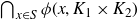
Proof. For the purpose of ensuring non-degeneracy, let
 $2\epsilon>0$
denote the minimal distance:
$2\epsilon>0$
denote the minimal distance:
 \begin{align*}\epsilon= \frac{1}{2} \min \left\{ |x^i- x^{j}|\,{:}\, i \neq j \in \{ 1, 2, \dots, k+1\} \right\}>0,\end{align*}
and, for each
 $i=1,2, \dots, k+1$
, define the
$i=1,2, \dots, k+1$
, define the
 $\epsilon$
-box about
$\epsilon$
-box about
 $x^i$
by
$x^i$
by
 \begin{align*}C(x^i, \epsilon)&= x^i + \left[\!- \epsilon,\epsilon\right]^2\\[3pt]&= \left[x^i_1 - \epsilon, x^i_1+\epsilon\right] \times \left[x^i_2- \epsilon, x^i_2+\epsilon\right]\\[3pt]&= C_1(x^i, \epsilon) \times C_2(x^i, \epsilon),\end{align*}
where
 $C_1(x^i, \epsilon), C_2(x^i, \epsilon)$
are the closed
$C_1(x^i, \epsilon), C_2(x^i, \epsilon)$
are the closed
 $\epsilon$
-intervals about the coordinates of
$\epsilon$
-intervals about the coordinates of
 $x^i$
(Figure 1).
$x^i$
(Figure 1).

Fig. 1. Boxes
 $C(x^i,\epsilon)$
around points
$C(x^i,\epsilon)$
around points
 $x^1,...,x^5$
.
$x^1,...,x^5$
.
Next, choose any leaf of T; without loss of generality we may assume we have labeled the vertices so that
 $k+1$
is our leaf. Let i denote the unique vertex which satisfies
$k+1$
is our leaf. Let i denote the unique vertex which satisfies
 $i\sim k+1$
. Let
$i\sim k+1$
. Let
 $\widetilde{K_j} = K_j \cap C_j(x^{k+1}, \epsilon)$
. By assumption, there exists a neighbourhood
$\widetilde{K_j} = K_j \cap C_j(x^{k+1}, \epsilon)$
. By assumption, there exists a neighbourhood
 $S_{i}$
of
$S_{i}$
of
 $x^{i}$
so that the set
$x^{i}$
so that the set
 \begin{equation} \bigcap_{x\in S_{i}}\phi(x,\widetilde{ K_1 }\times \widetilde{K_2})\end{equation}
has non-empty interior. Further, we may assume
 $S_{i}\subset C(x^{i},\epsilon)$
, which guarantees that the points in
$S_{i}\subset C(x^{i},\epsilon)$
, which guarantees that the points in
 $S_{i}$
and points in
$S_{i}$
and points in
 $\widetilde{K_1}\times \widetilde{K_2}\subset C(x^{k+1}, \epsilon)$
are distinct. Moreover, we can choose
$\widetilde{K_1}\times \widetilde{K_2}\subset C(x^{k+1}, \epsilon)$
are distinct. Moreover, we can choose
 $\epsilon_{2} \in (0, \epsilon]$
so that
$\epsilon_{2} \in (0, \epsilon]$
so that
 $C(x^i,\epsilon_{2}) \subset S_{i}$
, and hence (2·1) still holds with
$C(x^i,\epsilon_{2}) \subset S_{i}$
, and hence (2·1) still holds with
 $C(x^{i},\epsilon_2) $
in place of
$C(x^{i},\epsilon_2) $
in place of
 $S_{i}$
. For simplicity, we replace each of the
$S_{i}$
. For simplicity, we replace each of the
 $\epsilon$
-boxes about
$\epsilon$
-boxes about
 $x^{1}, \dots, x^{k+1}$
by potentially smaller boxes
$x^{1}, \dots, x^{k+1}$
by potentially smaller boxes
 $C(x^{j}, \epsilon_2)$
for each
$C(x^{j}, \epsilon_2)$
for each
 $j \in \{1, \dots, k+1\}$
.
$j \in \{1, \dots, k+1\}$
.
To conclude, let
 $E_{i} = C(x^{i},\epsilon_2)\cap (K_1\times K_2)$
, let
$E_{i} = C(x^{i},\epsilon_2)\cap (K_1\times K_2)$
, let
 $T_2$
be the tree obtained from T by removing the vertex
$T_2$
be the tree obtained from T by removing the vertex
 $k+1$
and its corresponding edge, and let
$k+1$
and its corresponding edge, and let
 $\Phi_2$
be the function as in the statement of the theorem, corresponding to the tree
$\Phi_2$
be the function as in the statement of the theorem, corresponding to the tree
 $T_2$
. We have proved there exists a non-empty open interval
$T_2$
. We have proved there exists a non-empty open interval
 $I_{1}$
so that
$I_{1}$
so that
 \begin{align*}\Phi(E_1\times\cdots\times E_{k+1})\supset \Phi_2(E_1\times\cdots\times E_k)\times I_1.\end{align*}
Running this argument successively on each of the trees
 $T_1,T_2,...,T_k$
as in Proposition 1·6, we conclude that
$T_1,T_2,...,T_k$
as in Proposition 1·6, we conclude that
 $\Phi((K_1\times K_2)^{k+1})$
contains a set of the form
$\Phi((K_1\times K_2)^{k+1})$
contains a set of the form
 $I_1\times \dots\times I_k$
for non-empty open intervals
$I_1\times \dots\times I_k$
for non-empty open intervals
 $I_1, \dots, I_k$
. By construction, it is clear that
$I_1, \dots, I_k$
. By construction, it is clear that
 $\Phi(x^1,...,x^{k+1})$
is in the closure of
$\Phi(x^1,...,x^{k+1})$
is in the closure of
 $I_1\times\cdots\times I_k$
.
$I_1\times\cdots\times I_k$
.
From the statement of Theorem 2·4, we see that we may start with any points
 $x^1,\dots,x^{k+1}\in K_1\times K_2$
and obtain an open box near
$x^1,\dots,x^{k+1}\in K_1\times K_2$
and obtain an open box near
 $\Phi\left(x^1,\dots,x^{k+1}\right)$
, provided we can prove pin wiggling lemmas around those points. We will refer to the starting points
$\Phi\left(x^1,\dots,x^{k+1}\right)$
, provided we can prove pin wiggling lemmas around those points. We will refer to the starting points
 $x^1,\dots,x^{k+1}$
as a skeleton.
$x^1,\dots,x^{k+1}$
as a skeleton.
Remark 2·5. In light of Theorem 1·7, it would be interesting to demonstrate the existence of an interval I such that
 $I^k\subset \Delta_T(K\times K)$
, as is done in [
Reference Bennett, Iosevich and Taylor1, Reference Iosevich and Taylor17
] in the large Hausdorff dimension context. By Theorem 2·4, this amounts to showing there exists a skeleton
$I^k\subset \Delta_T(K\times K)$
, as is done in [
Reference Bennett, Iosevich and Taylor1, Reference Iosevich and Taylor17
] in the large Hausdorff dimension context. By Theorem 2·4, this amounts to showing there exists a skeleton
 $x^1,...,x^{k+1}\in K\times K$
such that the distances
$x^1,...,x^{k+1}\in K\times K$
such that the distances
 $|x^i-x^j|$
are constant for
$|x^i-x^j|$
are constant for
 $i\sim j$
and such that no two points of the skeleton share a coordinate. It is not clear how to do this in general.
$i\sim j$
and such that no two points of the skeleton share a coordinate. It is not clear how to do this in general.
In the special case where T is a k-chain, it is sufficient (but not necessary) that K contains a length
 $k+1$
arithmetic progression. Given an arithmetic progression
$k+1$
arithmetic progression. Given an arithmetic progression
 $a_1,...,a_{k+1}\in K$
, we could then take
$a_1,...,a_{k+1}\in K$
, we could then take
 $x^i=(a_i,a_i)$
. Yavicoli [
Reference Yavicoli25
] shows that long arithmetic progressions exist in (very) thick Cantor sets. However, the required lower bound on thickness is much larger then the
$x^i=(a_i,a_i)$
. Yavicoli [
Reference Yavicoli25
] shows that long arithmetic progressions exist in (very) thick Cantor sets. However, the required lower bound on thickness is much larger then the
 $\tau(K)>1$
assumption in our results; to ensure even a 3-term arithmetic progression, one needs
$\tau(K)>1$
assumption in our results; to ensure even a 3-term arithmetic progression, one needs
 $\tau(K)$
at least on the order of
$\tau(K)$
at least on the order of
 $10^9$
. Moreover, Broderick, Fishman and Simmons [
Reference Broderick, Fishman and Simmons3
] prove that there is no arithmetic progression in
$10^9$
. Moreover, Broderick, Fishman and Simmons [
Reference Broderick, Fishman and Simmons3
] prove that there is no arithmetic progression in
 $C_\epsilon$
of length greater than
$C_\epsilon$
of length greater than
 ${1}/{\epsilon}+1$
for
${1}/{\epsilon}+1$
for
 $\epsilon$
sufficiently small, (where
$\epsilon$
sufficiently small, (where
 $C_\epsilon$
denotes the middle-
$C_\epsilon$
denotes the middle-
 $\epsilon$
Cantor set, obtained by starting with the unit interval and at each stage deleting the middle
$\epsilon$
Cantor set, obtained by starting with the unit interval and at each stage deleting the middle
 $\epsilon$
proportion from the remaining intervals). In particular, it follows that there is no
$\epsilon$
proportion from the remaining intervals). In particular, it follows that there is no
 $(k+1)$
progression in the set
$(k+1)$
progression in the set
 $C_{2/k}$
.
$C_{2/k}$
.
An alternative approach is to seek a common interval using the 2-dimensionality of
 $K\times K$
instead of hoping to take a sequence of points along the diagonal, and we address this in the sequel - see [
Reference McDonald and Taylor19
].
$K\times K$
instead of hoping to take a sequence of points along the diagonal, and we address this in the sequel - see [
Reference McDonald and Taylor19
].
3. Pin wiggling lemmas in various contexts
The proofs in this section are presented in increasing order of complexity.
3·1. Proof of Theorem 9·9
We begin by proving our result on dot product trees. As discussed in the introduction, dot products are much simpler than distances because thickness is preserved under affine transformations. As a consequence, Theorem 1·9 is the simplest of our results.
Theorem 1·9 is an immediate consequence of Theorem 2·4 and the following lemma.
Lemma 3·1 (Pin wiggling for dot products). Let
 $K_1,K_2$
be Cantor sets satisfying
$K_1,K_2$
be Cantor sets satisfying
 $\tau(K_1)\cdot \tau(K_2) \geq 1$
. Let
$\tau(K_1)\cdot \tau(K_2) \geq 1$
. Let
 $\ell_j$
denote the length of the convex hull of
$\ell_j$
denote the length of the convex hull of
 $K_j$
.
$K_j$
.
-
(i) For any
 $x=(x_1,x_2)\in \mathbb{R}^2$
with both coordinates nonzero, the set
$\Pi_x(K_1\times K_2)$
contains an interval of length at least
$\cdot\min\!(\ell_1|x_1|,\ell_2|x_2|)$
.
$x=(x_1,x_2)\in \mathbb{R}^2$
with both coordinates nonzero, the set
$\Pi_x(K_1\times K_2)$
contains an interval of length at least
$\cdot\min\!(\ell_1|x_1|,\ell_2|x_2|)$
. -
(ii) Let
$x^0=(x_1^0,x_2^0)\in \mathbb{R}^2$
be a point with both coordinates nonzero. Let Q be the square centered at
$x^0$
with side length
$2\delta$
, and assume
$\delta<\frac{1}{3}\min(|x_1^0|,|x_2^0|)$
. The set
contains an interval of length at least
\begin{align*}\bigcap_{x\in Q}\Pi_x(K_1\times K_2)\end{align*}
\begin{align*}\min\{\ell_2|x_2^0|-(\ell_2+2\ell_1)\delta,\ell_1|x_1^0|-(\ell_1+2\ell_2)\delta\}.\end{align*}


Proof. For any
 $x=(x^1, x^2)\in \mathbb{R}^2$
, we have
$x=(x^1, x^2)\in \mathbb{R}^2$
, we have
 $t\in \Pi_x(K_1\times K_2)$
if and only if
$t\in \Pi_x(K_1\times K_2)$
if and only if
 $(t-x_1K_1)\cap (x_2K_2)\neq\phi$
. Since
$(t-x_1K_1)\cap (x_2K_2)\neq\phi$
. Since
 $\tau(t-x_1K_1)\cdot \tau(x_2K_2)=\tau(K_1)\cdot \tau(K_2)\geq 1$
, by the Newhouse gap lemma, this intersection will be non-empty for any x and t such that the sets
$\tau(t-x_1K_1)\cdot \tau(x_2K_2)=\tau(K_1)\cdot \tau(K_2)\geq 1$
, by the Newhouse gap lemma, this intersection will be non-empty for any x and t such that the sets
 $(t-x_1K_1)$
and
$(t-x_1K_1)$
and
 $x_2K_2$
are linked. Denote the convex hull of
$x_2K_2$
are linked. Denote the convex hull of
 $x_jK_j$
by
$x_jK_j$
by
 $[a_j,a_j+\ell|x_j|]$
, and without loss of generality assume
$[a_j,a_j+\ell|x_j|]$
, and without loss of generality assume
 $\ell_1|x_1|\geq \ell_2|x_2|$
. The sets
$\ell_1|x_1|\geq \ell_2|x_2|$
. The sets
 $t-x_1K$
and
$t-x_1K$
and
 $x_2K$
are linked whenever
$x_2K$
are linked whenever
 \begin{align}a_1+a_2+\ell_1 |x_1|<t<a_1+a_2+\ell_1 |x_1|+\ell_2 |x_2|.\end{align}
The set of t satisfying (
 $*$
) is an interval of length
$*$
) is an interval of length
 $\ell_2 |x_2|$
, and so (i) follows immediately. To prove (ii), assume
$\ell_2 |x_2|$
, and so (i) follows immediately. To prove (ii), assume
 $(x_1,x_2)\in Q$
and therefore
$(x_1,x_2)\in Q$
and therefore
 $|x_j-x_j^0|<\delta$
for each j. The value t satisfies (
$|x_j-x_j^0|<\delta$
for each j. The value t satisfies (
 $*$
) for all such
$*$
) for all such
 $x_1,x_2$
provided
$x_1,x_2$
provided
 \begin{align*}a_1+a_2+\ell_1 |x_1^0|+\ell_1\delta<t<a_1+a_2+\ell_1 |x_1^0|+\ell_2 |x_2^0|-\ell_1\delta-\ell_2\delta.\end{align*}
This inequality determines an interval of length
 $\ell_2|x_2^0|-(\ell_2+2\ell_1)\delta$
.
$\ell_2|x_2^0|-(\ell_2+2\ell_1)\delta$
.
Note that when we apply Theorem 2·4, we can start with any skeleton
 $x^1,\dots,x^{k+1}\in K\times K$
such that none of the points
$x^1,\dots,x^{k+1}\in K\times K$
such that none of the points
 $x^i$
are on the axes.
$x^i$
are on the axes.
3·2. Proof of Theorem 1·7
As in the previous section, the proof will rely on the mechanism established in Theorem 2·4 coupled with a pin wiggling lemma. The difference is that the lemma of this section will not follow directly from the linear theory and some preliminary set up is required.
First, observe that given a pin
 $x\in \mathbb{R}^2$
and distance
$x\in \mathbb{R}^2$
and distance
 $t\in \mathbb{R}$
, we have
$t\in \mathbb{R}$
, we have
 $t\in \Delta_x(K\times K)$
whenever
$t\in \Delta_x(K\times K)$
whenever
 $y_2=g_{x,t}(y_1)$
for some
$y_2=g_{x,t}(y_1)$
for some
 $y = (y_1, y_2) \in K\times K$
, where
$y = (y_1, y_2) \in K\times K$
, where
 \begin{align*}g_{x,t}(z)=x_2+\sqrt{t^2-(z-x_1)^2}.\end{align*}
We would like to apply the Newhouse gap lemma to K and
 $g_{x,t}(K)$
to prove a pin wiggling lemma for distance sets (Lemma 3·5 below), then conclude that Theorem 1·7 follows (by Theorem 2·4). However, there is no thickness assumption on K which would guarantee
$g_{x,t}(K)$
to prove a pin wiggling lemma for distance sets (Lemma 3·5 below), then conclude that Theorem 1·7 follows (by Theorem 2·4). However, there is no thickness assumption on K which would guarantee
 $\tau(g_{x,t}(K))\geq 1$
, so we cannot apply Newhouse directly. However, if I is a sufficiently small interval about a non-singular point of
$\tau(g_{x,t}(K))\geq 1$
, so we cannot apply Newhouse directly. However, if I is a sufficiently small interval about a non-singular point of
 $g_{x,t}$
, then the thickness of
$g_{x,t}$
, then the thickness of
 $g_{x,t}(K\cap I)$
is not too much smaller than that of K. This can be proved using a generalization of thickness which was introduced in [
Reference Simon and Taylor23
], which we describe here.
$g_{x,t}(K\cap I)$
is not too much smaller than that of K. This can be proved using a generalization of thickness which was introduced in [
Reference Simon and Taylor23
], which we describe here.
Definition 3·2 (
 $\epsilon$
-thickness). Let
$\epsilon$
-thickness). Let
 $K\subset\mathbb{R}$
be a Cantor set, let u be a right endpoint of a bounded gap, G, and let
$K\subset\mathbb{R}$
be a Cantor set, let u be a right endpoint of a bounded gap, G, and let
 $\epsilon>0$
. Let (a, b) be the closest gap to G with the property that
$\epsilon>0$
. Let (a, b) be the closest gap to G with the property that
 $a>u$
and
$a>u$
and
 $(b-a)>(1-\epsilon)|G|$
. The
$(b-a)>(1-\epsilon)|G|$
. The
 $\epsilon$
-bridge of u, denoted
$\epsilon$
-bridge of u, denoted
 $B_\epsilon(u)$
, is the interval (u, a). We make analogous definitions for left endpoints. The
$B_\epsilon(u)$
, is the interval (u, a). We make analogous definitions for left endpoints. The
 $\epsilon$
-thickness of K at u is the quantity
$\epsilon$
-thickness of K at u is the quantity
 \begin{align*}\tau_\epsilon(K,u)\,{:\!=}\, \frac{|B_\epsilon(u)|}{|G|}.\end{align*}
Finally, the
 $\epsilon$
-thickness of the Cantor set K is the quantity
$\epsilon$
-thickness of the Cantor set K is the quantity
 \begin{align*}\tau_\epsilon(K)\,{:\!=}\,\inf_u \tau_\epsilon(K,u),\end{align*}
where the infimum is taken over all gap endpoints u.
We record some easily verifiable properties of
 $\epsilon$
-thickness in the following proposition.
$\epsilon$
-thickness in the following proposition.
Proposition 3·3 (
 $\epsilon$
-thickness converges to regular thickness). Let
$\epsilon$
-thickness converges to regular thickness). Let
 $K\subset \mathbb{R}$
be a Cantor set.
$K\subset \mathbb{R}$
be a Cantor set.
-
(i) If
$\epsilon_1<\epsilon_2$
then
$\tau_{\epsilon_1}(K)\geq \tau_{\epsilon_2}(K)$
. -
(ii)
$\tau_\epsilon(K)\to \tau(K)$
as
$\epsilon\to 0$
.


With these definitions in place, we can prove that the image of a thick Cantor set must at least contain a thick Cantor set. More precisely, we have the following lemma, which is essentially [ Reference Simon and Taylor23 , lemma 3·8]. We include a proof here for completeness.
Lemma 3·4 (Thickness of the image is nearly preserved). Let
 $K\subset\mathbb{R}$
be a Cantor set, let u be a right endpoint of some gap of K, and let g be a function which is continuously differentiable on a neighbourhood of u and satisfies
$K\subset\mathbb{R}$
be a Cantor set, let u be a right endpoint of some gap of K, and let g be a function which is continuously differentiable on a neighbourhood of u and satisfies
 $g'(u)\neq 0$
. For every
$g'(u)\neq 0$
. For every
 $\epsilon>0$
, there exists
$\epsilon>0$
, there exists
 $\delta>0$
such that
$\delta>0$
such that
 \begin{align*}\tau(g(K\cap [u,u+\delta]))>\tau_\epsilon(K)(1-\epsilon).\end{align*}
Proof. Fix
 $\epsilon>0$
. By continuity of g
$\epsilon>0$
. By continuity of g
 $^{\prime}$
, we may choose
$^{\prime}$
, we may choose
 $\delta$
such that for all
$\delta$
such that for all
 $x_1,x_2\in[u,u+\delta]$
we have
$x_1,x_2\in[u,u+\delta]$
we have
 \begin{align*}\left|\frac{g'(x_1)}{g'(x_2)}-1\right|<\epsilon.\end{align*}
Note that our choice of
 $\delta$
guarantees that g is monotone on the interval
$\delta$
guarantees that g is monotone on the interval
 $[u,u+\delta]$
, so for any subinterval I the mean value theorem guarantees the existence of some
$[u,u+\delta]$
, so for any subinterval I the mean value theorem guarantees the existence of some
 $x_I\in I$
such that
$x_I\in I$
such that
 $|g(I)|=|I|\cdot |g'(x_I)|$
. Let v be the endpoint of some gap G in
$|g(I)|=|I|\cdot |g'(x_I)|$
. Let v be the endpoint of some gap G in
 $K\cap [u,u+\delta]$
. We first observe
$K\cap [u,u+\delta]$
. We first observe
 $g(B_\epsilon(v))\subset B_{\epsilon^2}(g(v))$
. To prove this, note that any gap in
$g(B_\epsilon(v))\subset B_{\epsilon^2}(g(v))$
. To prove this, note that any gap in
 $g(K\cap [u,u+\delta])$
is the image of a gap in
$g(K\cap [u,u+\delta])$
is the image of a gap in
 $K\cap [u,u+\delta]$
. Therefore, it suffices to prove that any gap
$K\cap [u,u+\delta]$
. Therefore, it suffices to prove that any gap
 $H\subset B_\epsilon(v)$
satisfies
$H\subset B_\epsilon(v)$
satisfies
 $|g(H)|<(1-\epsilon^2)|g(G)|$
. To this end, observe that if H is a gap in
$|g(H)|<(1-\epsilon^2)|g(G)|$
. To this end, observe that if H is a gap in
 $B_\epsilon(v)$
, then
$B_\epsilon(v)$
, then
 $|H| \le (1-\epsilon)|G|$
, and we have
$|H| \le (1-\epsilon)|G|$
, and we have
 \begin{align*}|g(H)|&=|H|\cdot |g'(x_H)| \\&\le(1-\epsilon)|G|\cdot\frac{|g'(x_H)|}{|g'(x_G)|}\cdot |g'(x_G)| \\&<(1-\epsilon)|G|\cdot (1+\epsilon)\cdot |g'(x_G)| \\&=(1-\epsilon^2)|g(G)|.\end{align*}
It follows by definition then that the thickness of the image at the point g(v) satisfies
 \begin{align*}\tau_{\epsilon^2}(g(K\cap[u,u+\delta]),g(v)) &\geq \frac{|g(B_\epsilon(v))|}{|g(G)|}\\&=\frac{|B_\epsilon(v)|}{|G|}\cdot \left|\frac{g'(x_{B_\epsilon(v)} )}{g'(x_G)}\right| \\&> \tau_\epsilon(K\cap[u,u+\delta],v)\cdot(1-\epsilon).\end{align*}
Taking the infimum over v, we have
 \begin{align*}\tau(g(K\cap[u,u+\delta]))\geq \tau_{\epsilon^2}(g(K\cap[u,u+\delta])) > \tau_\epsilon(K)(1-\epsilon).\end{align*}
This completes the proof of the lemma.
We are now prepared to state and prove the key lemma for distances.
Lemma 3·5 (Pin wiggling for distances). Let
 $K_1,K_2$
be Cantor sets satisfying
$K_1,K_2$
be Cantor sets satisfying
 $\tau(K_1)\cdot \tau(K_2) > 1$
. For any
$\tau(K_1)\cdot \tau(K_2) > 1$
. For any
 $x^0\in \mathbb{R}^2$
, there exists an open S about
$x^0\in \mathbb{R}^2$
, there exists an open S about
 $x^0$
so that
$x^0$
so that
 \begin{align*}\bigcap_{x\in S} \Delta_{x}(K_1\times K_2)\end{align*}
has non-empty interior.
Proof. For
 $(x,t)\in\mathbb{R}^2\times (0,\infty)$
, define
$(x,t)\in\mathbb{R}^2\times (0,\infty)$
, define
 \begin{equation}g_{x,t}(z)=x_2+\sqrt{t^2-(z-x_1)^2},\end{equation}
and observe that
 $t\in\Delta_{x}(K_1\times K_2)$
provided
$t\in\Delta_{x}(K_1\times K_2)$
provided
 $K_2\cap g_{x,t}(K_1)\neq\phi$
. Let
$K_2\cap g_{x,t}(K_1)\neq\phi$
. Let
 $u_j$
be a right endpoint of a bounded gap of
$u_j$
be a right endpoint of a bounded gap of
 $K_j$
, and without loss of generality assume
$K_j$
, and without loss of generality assume
 $u_j>x_j^0$
, where
$u_j>x_j^0$
, where
 $x^0 = \left(x^0_1, x^0_2\right)$
. We choose small subsets
$x^0 = \left(x^0_1, x^0_2\right)$
. We choose small subsets
 $\widetilde{K_j}\subset K_j$
with left endpoint
$\widetilde{K_j}\subset K_j$
with left endpoint
 $u_j$
, and focus on the box
$u_j$
, and focus on the box
 $\widetilde{K_1}\times \widetilde{K_2}$
(Figure 2). Let
$\widetilde{K_1}\times \widetilde{K_2}$
(Figure 2). Let
 $t_0=|x^0-(u_1,u_2)|$
. Let
$t_0=|x^0-(u_1,u_2)|$
. Let
 $\widetilde{K_j}=K_j\cap[u_j,u_j+\delta_j]$
for some small
$\widetilde{K_j}=K_j\cap[u_j,u_j+\delta_j]$
for some small
 $\delta_1,\delta_2$
. In particular, we choose
$\delta_1,\delta_2$
. In particular, we choose
 $\delta_j>0$
small enough that
$\delta_j>0$
small enough that
 $\tau(\widetilde{K_2})\cdot \tau(g(\widetilde{K_1}))>1$
(this is possible by Lemma 3·4), and so that
$\tau(\widetilde{K_2})\cdot \tau(g(\widetilde{K_1}))>1$
(this is possible by Lemma 3·4), and so that
 $\widetilde{K_1}$
is in the domain of
$\widetilde{K_1}$
is in the domain of
 $g_{x,t}$
whenever (x, t) is sufficiently close to
$g_{x,t}$
whenever (x, t) is sufficiently close to
 $(x^0,t_0)$
. We will also assume
$(x^0,t_0)$
. We will also assume
 $u_j+\delta_j\in K_j$
.
$u_j+\delta_j\in K_j$
.
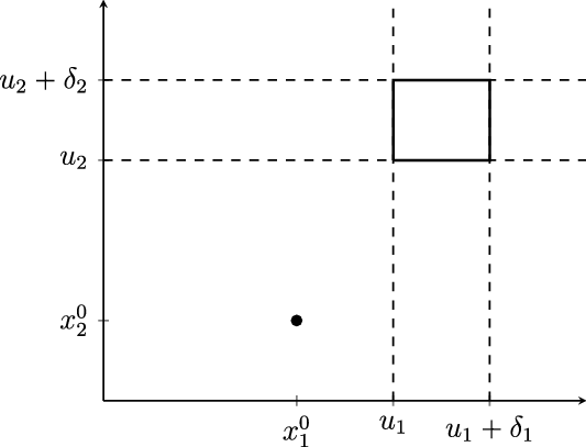
Fig. 2. The box containing
 $\widetilde{K_1}\times \widetilde{K_2}$
.
$\widetilde{K_1}\times \widetilde{K_2}$
.
By the Newhouse gap lemma (Proposition 2·3), we will have
 $\widetilde{K_2}\cap g_{x,t}(\widetilde{K_1})\neq\phi$
whenever the parameters (x, t) are such that
$\widetilde{K_2}\cap g_{x,t}(\widetilde{K_1})\neq\phi$
whenever the parameters (x, t) are such that
 $\widetilde{K_2}$
and
$\widetilde{K_2}$
and
 $g_{x,t}(\widetilde{K_1})$
are linked. To this end, consider the set
$g_{x,t}(\widetilde{K_1})$
are linked. To this end, consider the set
 \begin{align*}U=\{(x,t)\in\mathbb{R}^2\times\mathbb{R}\,{:}\,g_{x,t}(u_1+\delta_1)<u_2<g_{x,t}(u_1)<u_2+\delta_2\}.\end{align*}
By construction, for any
 $(x,t)\in U$
we have
$(x,t)\in U$
we have
 $K_2$
and
$K_2$
and
 $g_{x,t}(K_1)$
linked (Figure 3) and hence
$g_{x,t}(K_1)$
linked (Figure 3) and hence
 $t\in\Delta_x(K_1\times K_2)$
. We claim that U is an open set containing a point of the form
$t\in\Delta_x(K_1\times K_2)$
. We claim that U is an open set containing a point of the form
 $(x^0,t)$
for some t. Lemma 3·5 follows from this claim, as we can then take open neighbourhoods S, T of
$(x^0,t)$
for some t. Lemma 3·5 follows from this claim, as we can then take open neighbourhoods S, T of
 $x^0,t$
respectively such that
$x^0,t$
respectively such that
 \begin{align*}T\subset \bigcap_{x\in S} \Delta_{x}(K_1\times K_2).\end{align*}
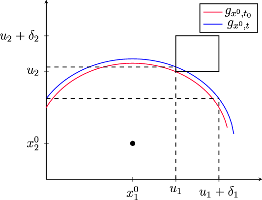
Fig. 3. Graphs of g.
To prove the claim, we first observe that U is open, since for fixed z the quantity
 $g_{x,t}(z)$
is a continuous function of (x, t). To finish the proof, we must find a t such that
$g_{x,t}(z)$
is a continuous function of (x, t). To finish the proof, we must find a t such that
 $(x^0,t)\in U$
. By construction, we have
$(x^0,t)\in U$
. By construction, we have
 $g_{x^0,t_0}(u_1)=u_2$
. Since the quantity
$g_{x^0,t_0}(u_1)=u_2$
. Since the quantity
 $g_{x,t}(z)$
is strictly increasing in t, for any
$g_{x,t}(z)$
is strictly increasing in t, for any
 $t>t_0$
we will have
$t>t_0$
we will have
 $g_{x^0,t}(u_1)>u_2$
. On the other hand, by continuity in t we will also have
$g_{x^0,t}(u_1)>u_2$
. On the other hand, by continuity in t we will also have
 $g_{x^0,t}(u_1+\delta_1)<u_2$
and
$g_{x^0,t}(u_1+\delta_1)<u_2$
and
 $g_{x^0,t}(u_1)<u_2+\delta_2$
whenever t is sufficiently close to
$g_{x^0,t}(u_1)<u_2+\delta_2$
whenever t is sufficiently close to
 $t_0$
. Therefore, we can choose t with the property that
$t_0$
. Therefore, we can choose t with the property that
 $(x^0,t_0)\in U$
.
$(x^0,t_0)\in U$
.
Theorem 1·7 follows from Lemma 3·5 and Theorem 2·4. Note that when we apply Theorem 2·4, we can start with any skeleton
 $x^1,\dots,x^{k+1}\in K_1\times K_2$
provided no two points
$x^1,\dots,x^{k+1}\in K_1\times K_2$
provided no two points
 $x^i,x^j$
share a coordinate.
$x^i,x^j$
share a coordinate.
3·3. Proof of Theorem 1·14
As in the previous two sections, Theorem 1·14 on
 $\phi$
distance trees is an immediate consequence of Theorem 2·4 and the following lemma.
$\phi$
distance trees is an immediate consequence of Theorem 2·4 and the following lemma.
Lemma 3·6 (Pin wiggling for
 $\phi$
distance trees). Let
$\phi$
distance trees). Let
 $K_1,K_2$
be Cantor sets satisfying
$K_1,K_2$
be Cantor sets satisfying
 $\tau(K_1)\cdot \tau(K_2) > 1$
Suppose
$\tau(K_1)\cdot \tau(K_2) > 1$
Suppose
 $\phi\,{:}\,\mathbb{R}^2 \times \mathbb{R}^2 \rightarrow \mathbb{R}$
satisfies the derivative condition of Definition 1·12 on
$\phi\,{:}\,\mathbb{R}^2 \times \mathbb{R}^2 \rightarrow \mathbb{R}$
satisfies the derivative condition of Definition 1·12 on
 $A\times B$
for open
$A\times B$
for open
 $A,B\subset \mathbb{R}^2$
, each of which intersects
$A,B\subset \mathbb{R}^2$
, each of which intersects
 $K_1\times K_2$
. For any
$K_1\times K_2$
. For any
 $x^0 \in A$
, there exists an open S about
$x^0 \in A$
, there exists an open S about
 $x^0$
so that
$x^0$
so that
 \begin{align*}\bigcap_{x\in S} \Delta_{\phi, x}(K_1\times K_2)\end{align*}
has non-empty interior, where
 $\Delta_{\phi, x}(K_1\times K_2) = \{ \phi(x,y)\,{:}\, y \in K_1\times K_2\}.$
The strategy for establishing Lemma 3·6 is as follows: given a pin
 $x\in \mathbb{R}^2$
and distance
$x\in \mathbb{R}^2$
and distance
 $t\in \mathbb{R}$
, we note that
$t\in \mathbb{R}$
, we note that
 $t\in \Delta_{\phi,x}(K_1\times K_2)$
whenever
$t\in \Delta_{\phi,x}(K_1\times K_2)$
whenever
 $\phi(x,y) = t$
for some
$\phi(x,y) = t$
for some
 $y=(y_1,y_2)\in K_1\times K_2$
. We then use the implicit function theorem to solve for
$y=(y_1,y_2)\in K_1\times K_2$
. We then use the implicit function theorem to solve for
 $y_2$
in terms of
$y_2$
in terms of
 $(x, y_1,t)$
and call the resulting function g. Observing that g behaves like the function
$(x, y_1,t)$
and call the resulting function g. Observing that g behaves like the function
 $g_{x,t}$
introduced in the proof of Lemma 3·5 from the previous section, the lemma then follows from the exact proof used for Euclidean distances. The only real effort of the proof then is setting up the implicit function theorem.
$g_{x,t}$
introduced in the proof of Lemma 3·5 from the previous section, the lemma then follows from the exact proof used for Euclidean distances. The only real effort of the proof then is setting up the implicit function theorem.
Proof. Let
 $\varphi_x(y) = \phi(x,y)$
as in Definition 1·12 so that for all
$\varphi_x(y) = \phi(x,y)$
as in Definition 1·12 so that for all
 $(x,y) \in A\times B$
,
$(x,y) \in A\times B$
,
 \begin{equation}\frac{\partial (\varphi_x)}{\partial y_i} (y)\neq 0 \text{ for } i =1,2.\end{equation}
Define
 $F\,{:}\,\mathbb{R}^2\times \mathbb{R}^2 \times \mathbb{R} \rightarrow \mathbb{R}$
by
$F\,{:}\,\mathbb{R}^2\times \mathbb{R}^2 \times \mathbb{R} \rightarrow \mathbb{R}$
by
 \begin{equation}F(x, y,t) = \phi(x,y) -t.\end{equation}
Then F is continuously differentiable on
 $A\times B\times \mathbb{R}$
. Moreover, it follows by (3·2) that the partial derivative of F in
$A\times B\times \mathbb{R}$
. Moreover, it follows by (3·2) that the partial derivative of F in
 $y_2$
is non-vanishing on
$y_2$
is non-vanishing on
 $A\times B\times \mathbb{R}$
. Choose
$A\times B\times \mathbb{R}$
. Choose
 $x^0 \in A$
and
$x^0 \in A$
and
 $u=(u_1,u_2) \in B\cap (K_1 \times K_2)$
. Set
$u=(u_1,u_2) \in B\cap (K_1 \times K_2)$
. Set
 \begin{align*}t_0 = \phi\!\left( x^0, u\right)\end{align*}
so that
 \begin{align*}F\!\left(x^0,u, t_0\right) = 0.\end{align*}
By the implicit function theorem, there exists a real-valued function g and a
 $\delta$
-ball about the point
$\delta$
-ball about the point
 $(x^0, u_1, t_0)$
, denoted by
$(x^0, u_1, t_0)$
, denoted by
 $B_\delta= B_{\delta}(x^0, u_1, t_0)$
, so that:
$B_\delta= B_{\delta}(x^0, u_1, t_0)$
, so that:
-
(i) g is continuously differentiable on
$B_{\delta}$
; -
(ii)
$g(x^0,u_1, t_0) = u_2$
; -
(iii) if
$(x, y_1, t) \in B_{\delta}$
, then
$(x, y) \in A\times B$
for all
$y= (y_1, g(x,y_1, t) )$
; -
(iv)
$\phi(x, y) = t$
for all
$y= (y_1, g(x,y_1, t) ) $
when
$(x, y_1, t) \in B_{\delta}$
.


Moreover, if
 $g_{x,t}(y_1) = g(x,y_1, t)$
, then
$g_{x,t}(y_1) = g(x,y_1, t)$
, then
 \begin{align*}g_{x,t}^{\prime} (y_1) = -\left( \frac{\partial (\varphi_x)}{\partial y_1}(y_1, g(x, y_1, t))\right) / \left( \frac{\partial (\varphi_x)}{\partial y_2}(y_1, g(x, y_1, t))\right) \neq 0\end{align*}
for
 $(x, y_1, t) \in B_\delta= B_{\delta}(x^0,u_1, t_0)$
. In other words, there is a neighbourhood of
$(x, y_1, t) \in B_\delta= B_{\delta}(x^0,u_1, t_0)$
. In other words, there is a neighbourhood of
 $(x^0, t_0) $
so that the derivative of
$(x^0, t_0) $
so that the derivative of
 $g_{x,t}$
is non-vanishing in a neighbourhood of
$g_{x,t}$
is non-vanishing in a neighbourhood of
 $u_1$
.
$u_1$
.
Replacing the function in (3·1) of Lemma 3·5 with this new
 $g_{x,t}$
, the proof proceeds as in the proof of Lemma 3·5.
$g_{x,t}$
, the proof proceeds as in the proof of Lemma 3·5.
3·4. Distance trees in the middle thirds cantor set
In this section, we prove Theorem 1·10. The new twist in this context is that the middle thirds Cantor set has thickness equal to 1, not strictly greater than 1. Our method uses Lemma 3·4 which controls how much smaller the thickness of
 $g(\widetilde{K})$
can be compared to K, where
$g(\widetilde{K})$
can be compared to K, where
 $\widetilde{K}$
is a choosen subset of K. If
$\widetilde{K}$
is a choosen subset of K. If
 $\tau(K)=1$
, then we cannot assume
$\tau(K)=1$
, then we cannot assume
 $\tau(g(\widetilde{K}))\geq 1$
and therefore cannot apply the Newhouse gap lemma directly. However, the self similarity of the middle thirds Cantor set provides a tool that allows one to adapt the proof of the Newhouse gap lemma in this special setting. This observation was used in [
Reference Simon and Taylor23
] to prove that the pinned distance set
$\tau(g(\widetilde{K}))\geq 1$
and therefore cannot apply the Newhouse gap lemma directly. However, the self similarity of the middle thirds Cantor set provides a tool that allows one to adapt the proof of the Newhouse gap lemma in this special setting. This observation was used in [
Reference Simon and Taylor23
] to prove that the pinned distance set
 $\Delta_x(C_{1/3}\times C_{1/3})$
has non-empty interior. We use this idea to prove a pin wiggling lemma for the middle thirds Cantor set.
$\Delta_x(C_{1/3}\times C_{1/3})$
has non-empty interior. We use this idea to prove a pin wiggling lemma for the middle thirds Cantor set.
Before proceeding, we introduce some terminology. Let
 $C_{1/3}$
denote the standard middle thirds Cantor set in the interval [0, 1]. The standard construction of this set is given by defining
$C_{1/3}$
denote the standard middle thirds Cantor set in the interval [0, 1]. The standard construction of this set is given by defining
 $C_{1/3}$
as the intersection of a family of sets
$C_{1/3}$
as the intersection of a family of sets
 $\{C_n\}$
, where each
$\{C_n\}$
, where each
 $C_n$
is the union of
$C_n$
is the union of
 $2^n$
closed intervals of length
$2^n$
closed intervals of length
 $1/3^n$
. Define a section of
$1/3^n$
. Define a section of
 $C_{1/3}$
to be the intersection of
$C_{1/3}$
to be the intersection of
 $C_{1/3}$
with any one of the intervals making up any of the sets
$C_{1/3}$
with any one of the intervals making up any of the sets
 $C_n$
.
$C_n$
.
Lemma 3·7.
Let
 $K_1,K_2$
be sections of the standard middle thirds Cantor
$K_1,K_2$
be sections of the standard middle thirds Cantor
 $\mathcal{C}$
, and let g be a continuously differentiable monotone function which satisfies
$\mathcal{C}$
, and let g be a continuously differentiable monotone function which satisfies
 $1<g'<3$
on the convex hull of
$1<g'<3$
on the convex hull of
 $K_1$
. If
$K_1$
. If
 $K_2$
and
$K_2$
and
 $g(K_1)$
are linked, then
$g(K_1)$
are linked, then
 $K_2\cap g(K_1)\neq \phi$
.
$K_2\cap g(K_1)\neq \phi$
.
Proof. We begin with a simple observation. Let
 $I_1,I_2$
denote the convex hulls of
$I_1,I_2$
denote the convex hulls of
 $K_1, K_2$
, respectively. By the mean value theorem, for any interval J there exists
$K_1, K_2$
, respectively. By the mean value theorem, for any interval J there exists
 $x_J\in J$
such that
$x_J\in J$
such that
 $|g(J)|=|J|\cdot|g'(x_J)|$
. In particular, if U and V are bounded gaps of
$|g(J)|=|J|\cdot|g'(x_J)|$
. In particular, if U and V are bounded gaps of
 $K_1$
and
$K_1$
and
 $|U|>|V|$
, we have
$|U|>|V|$
, we have
 $|U|\geq 3|V|$
and therefore
$|U|\geq 3|V|$
and therefore
 \begin{align*}\\[-20pt]|g(U)|&=|U|\cdot |g'(x_U)| \\[3pt] &> 3|V|\cdot 1 \\[3pt] &> |g'(x_V)|\cdot |V| \\[3pt] &= |g(V)|.\end{align*}
It follows that the bridges of the images are the images of the bridges. More precisely, the bridge of gap g(U) in
 $g(K_1)$
is g(B), where B is the bridge next to the gap U.
$g(K_1)$
is g(B), where B is the bridge next to the gap U.
Now, to prove the lemma, we proceed by contradiction and assume
 $K_2\cap g(K_1)=\phi$
. The strategy of the proof is a variant of the strategy used to prove the original Newhouse gap lemma. We construct sequences of gaps
$K_2\cap g(K_1)=\phi$
. The strategy of the proof is a variant of the strategy used to prove the original Newhouse gap lemma. We construct sequences of gaps
 $U_n, V_n$
satisfying the following conditions:
$U_n, V_n$
satisfying the following conditions:
-
(i)
$U_n$
is a bounded gap of
$K_2$
and
$g(V_n)$
is a bounded gap of
$g(K_1)$
; -
(ii)
$U_n$
and
$g(V_n)$
are linked for every n; -
(iii) for every n, either
-
(a)
$U_{n+1}=U_n$
and
$|g(V_{n+1})|<|g(V_n)|$
, or -
(b)
$V_{n+1}=V_n$
and
$|U_{n+1}|<|U_n|$
.
-


Thus, at each stage we are replacing one of the gaps
 $U_n,g(V_n)$
with a strictly smaller one and leaving the other unchanged. In particular, this means that one of the two gap sequences must have a subsequence which is strictly decreasing in length. Since gaps of different sizes are automatically disjoint and the total length of the gaps is bounded, we must have either
$U_n,g(V_n)$
with a strictly smaller one and leaving the other unchanged. In particular, this means that one of the two gap sequences must have a subsequence which is strictly decreasing in length. Since gaps of different sizes are automatically disjoint and the total length of the gaps is bounded, we must have either
 $|U_n|\to 0$
or
$|U_n|\to 0$
or
 $|g(V_n)|\to 0$
as
$|g(V_n)|\to 0$
as
 $n\to\infty$
. However, because
$n\to\infty$
. However, because
 $U_n$
and
$U_n$
and
 $g(V_n)$
are linked, the closure of
$g(V_n)$
are linked, the closure of
 $U_n$
contains points of both
$U_n$
contains points of both
 $K_2$
and
$K_2$
and
 $g(K_1)$
, and similarly for
$g(K_1)$
, and similarly for
 $g(V_n)$
. This implies that the distance between
$g(V_n)$
. This implies that the distance between
 $K_2$
and
$K_2$
and
 $g(K_1)$
is zero, which contradicts the assumption
$g(K_1)$
is zero, which contradicts the assumption
 $K_2\cap g(K_1)= \phi$
.
$K_2\cap g(K_1)= \phi$
.
We construct our sequences
 $\{U_n\}$
and
$\{U_n\}$
and
 $\{V_n\}$
recursively. First, we construct
$\{V_n\}$
recursively. First, we construct
 $U_1$
and
$U_1$
and
 $V_1$
. Recall that
$V_1$
. Recall that
 $I_i$
denotes the convex hull of
$I_i$
denotes the convex hull of
 $K_i$
for
$K_i$
for
 $i=1,2$
. Since
$i=1,2$
. Since
 $I_2$
and
$I_2$
and
 $g(I_1)$
are linked by assumption, there is a bounded gap
$g(I_1)$
are linked by assumption, there is a bounded gap
 $U_1$
of
$U_1$
of
 $K_2$
which is a subset of
$K_2$
which is a subset of
 $I_2\cap g(I_1)$
. Let u be an endpoint of
$I_2\cap g(I_1)$
. Let u be an endpoint of
 $U_1$
. In particular we have
$U_1$
. In particular we have
 $u\in K_2$
, and therefore, by our assumption that
$u\in K_2$
, and therefore, by our assumption that
 $K_2\cap g(K_1)=\phi$
, it follows that u is in some bounded gap
$K_2\cap g(K_1)=\phi$
, it follows that u is in some bounded gap
 $g(V_1)$
of
$g(V_1)$
of
 $g(K_1)$
.
$g(K_1)$
.
Next, suppose we have constructed
 $U_n$
and
$U_n$
and
 $V_n$
satisfying the properties in the first two bullet points above. We construct
$V_n$
satisfying the properties in the first two bullet points above. We construct
 $U_{n+1}$
and
$U_{n+1}$
and
 $V_{n+1}$
satisfying the third bullet point. By construction,
$V_{n+1}$
satisfying the third bullet point. By construction,
 $U_n$
and
$U_n$
and
 $g(V_n)$
are linked. Let
$g(V_n)$
are linked. Let
 $B_n^U$
be the bridge corresponding to
$B_n^U$
be the bridge corresponding to
 $U_n$
on the same side as
$U_n$
on the same side as
 $g(V_n)$
(see Figure 4), and let
$g(V_n)$
(see Figure 4), and let
 $g\left(B_n^V\right)$
be the bridge of
$g\left(B_n^V\right)$
be the bridge of
 $g(V_n)$
on the same side as
$g(V_n)$
on the same side as
 $U_n$
. We claim that one of the following two inequalities must hold:
$U_n$
. We claim that one of the following two inequalities must hold:
 \begin{align*}|g(B_n^V)|&>|U_n| \\[4pt] |B_n^U|&>|g(V_n)|.\end{align*}
This follows because we are working with the middle thirds Cantor set, so bounded gaps and corresponding bridges have the same length, i.e., we have
 $|B_n^U|=|U_n|$
and
$|B_n^U|=|U_n|$
and
 $|B_n^V|=|V_n|.$
The middle thirds Cantor set also has the property that if U and V are gaps with
$|B_n^V|=|V_n|.$
The middle thirds Cantor set also has the property that if U and V are gaps with
 $|U|>|V|$
, we automatically have
$|U|>|V|$
, we automatically have
 $|U|\geq 3|V|$
. Finally, by our assumptions on g, we have
$|U|\geq 3|V|$
. Finally, by our assumptions on g, we have
 $|J|< |g(J)|< 3|J|$
for every interval
$|J|< |g(J)|< 3|J|$
for every interval
 $J\subset I_1$
. The claim then follows, as
$J\subset I_1$
. The claim then follows, as
 $|U_n|>|V_n|$
implies the second inequality and
$|U_n|>|V_n|$
implies the second inequality and
 $|U_n|\leq |V_n|$
implies the first.
$|U_n|\leq |V_n|$
implies the first.

Fig. 4. Construction of gap sequence (gaps are red, bridges are blue).
Assume the second inequality holds (an analogous argument will apply when the first holds). This means one endpoint of
 $g(V_n)$
is in
$g(V_n)$
is in
 $U_n$
and the other is in
$U_n$
and the other is in
 $B_n^U$
(see Figure 4 again). Recall that we are proving the lemma by contradiction, assuming
$B_n^U$
(see Figure 4 again). Recall that we are proving the lemma by contradiction, assuming
 $K_2\cap g(K_1)=\phi$
. This assumption means the endpoint of
$K_2\cap g(K_1)=\phi$
. This assumption means the endpoint of
 $g(V_n)$
which is in
$g(V_n)$
which is in
 $B_n^U$
must be contained in some gap
$B_n^U$
must be contained in some gap
 $U_{n+1}$
of
$U_{n+1}$
of
 $K_2$
, and by definition of a bridge we must have
$K_2$
, and by definition of a bridge we must have
 $|U_{n+1}|<|U_n|$
. We then take
$|U_{n+1}|<|U_n|$
. We then take
 $V_{n+1}=V_n$
. This completes the construction.
$V_{n+1}=V_n$
. This completes the construction.
Theorem 3·8.
Given a point
 $x^0\in \mathbb{R}^2$
, let
$x^0\in \mathbb{R}^2$
, let
 $W_{x^0}$
denote the open wedge
$W_{x^0}$
denote the open wedge
 \begin{align*}W_{x^0}=\left\{x\in\mathbb{R}^2\,{:}\,\left(x_2-x_2^0\right)<\left(x_1-x_1^0\right)<3\left(x_2-x_2^0\right)\right\}.\end{align*}
Let
 $K_1,K_2$
be sections of the middle thirds Cantor set, and suppose
$K_1,K_2$
be sections of the middle thirds Cantor set, and suppose
 $K_1\times K_2\subset W_{x^0}$
(Figure 5
). Then, there exists an open neighbourhood S of
$K_1\times K_2\subset W_{x^0}$
(Figure 5
). Then, there exists an open neighbourhood S of
 $x^0$
such that
$x^0$
such that
 \begin{align*}\bigcap_{x\in S}\Delta_x(K_1\times K_2)\end{align*}
has non-empty interior.

Fig. 5. The wedge of acceptable boxes.
Proof. For
 $x\in\mathbb{R}^2$
and
$x\in\mathbb{R}^2$
and
 $t\in\mathbb{R}$
, consider the function
$t\in\mathbb{R}$
, consider the function
 \begin{align*}g_{x,t}(z)=x_2+\sqrt{t^2-(z-x_1)^2}.\end{align*}
We have
 \begin{align*}g_{x,t}^{\prime}(z)=-\frac{z-x_1}{g_{x,t}(z)-x_2},\end{align*}
so
 $1<|g_{x,t}^{\prime}(z)|<3$
whenever
$1<|g_{x,t}^{\prime}(z)|<3$
whenever
 $(z,g_{x,t}(z))\in W_x$
. For
$(z,g_{x,t}(z))\in W_x$
. For
 $j=1,2$
, let
$j=1,2$
, let
 $u_j=\min K_j$
, so that
$u_j=\min K_j$
, so that
 $u=(u_1,u_2)$
denotes the lower left corner of
$u=(u_1,u_2)$
denotes the lower left corner of
 $K_1\times K_2$
, and let
$K_1\times K_2$
, and let
 $t_0=|x^0-u|$
(thus, we have
$t_0=|x^0-u|$
(thus, we have
 $g_{x^0,t_0}(u_1)=u_2$
). For every
$g_{x^0,t_0}(u_1)=u_2$
). For every
 $\delta>0$
, define
$\delta>0$
, define
 $\widetilde{K_j}=K_j\cap [u_1,u_1+\delta]$
and consider the set
$\widetilde{K_j}=K_j\cap [u_1,u_1+\delta]$
and consider the set
 \begin{align*}U_\delta=\{(x,t) \,{:}\,\widetilde{K_2}\text{ and }g_{x,t}(\widetilde{K_1}) \text{ are linked, and }(z,g_{x,t}(z))\in W_x \text{ for all }z\in[u_1,u_1+\delta]\}.\end{align*}
By Lemma 3·7, if
 $(x,t)\in U_\delta$
then
$(x,t)\in U_\delta$
then
 $t\in \Delta_x(K_1\times K_2)$
. Clearly
$t\in \Delta_x(K_1\times K_2)$
. Clearly
 $U_\delta$
is open, so as in the previous proofs it suffices to show that
$U_\delta$
is open, so as in the previous proofs it suffices to show that
 $U_\delta$
contains a point of the form
$U_\delta$
contains a point of the form
 $(x^0,t)$
. We first observe that if
$(x^0,t)$
. We first observe that if
 $\delta$
is sufficiently small, the sets
$\delta$
is sufficiently small, the sets
 $\widetilde{K_2}$
and
$\widetilde{K_2}$
and
 $g_{x,t}(\widetilde{K_1})$
are linked for all
$g_{x,t}(\widetilde{K_1})$
are linked for all
 $t\in(t_0,t_0+\delta)$
. This is because for any
$t\in(t_0,t_0+\delta)$
. This is because for any
 $t>t_0$
we have
$t>t_0$
we have
 $g_{x^0,t}(u_1)>u_2$
, and for any
$g_{x^0,t}(u_1)>u_2$
, and for any
 $t<u_1+\delta$
we will also have
$t<u_1+\delta$
we will also have
 $g_{x^0,t}(u_1)\gt u_2+\delta$
and
$g_{x^0,t}(u_1)\gt u_2+\delta$
and
 $g_{x^0,t}(u_1+\delta)\gt u_2$
. Finally, since
$g_{x^0,t}(u_1+\delta)\gt u_2$
. Finally, since
 $u\in W_{x^0}$
by assumption, if
$u\in W_{x^0}$
by assumption, if
 $\delta'$
is sufficiently small we will have
$\delta'$
is sufficiently small we will have
 $(z,g_{x^0,t}(z))\in W_{x^0}$
for all
$(z,g_{x^0,t}(z))\in W_{x^0}$
for all
 $z\in [u_1,u_1+\delta]$
and all
$z\in [u_1,u_1+\delta]$
and all
 $t\in (t_0,t_0+\delta')$
.
$t\in (t_0,t_0+\delta')$
.
Proof of Theorem 1·10. By Theorem 2·4, it suffices to find a skeleton
 $x^1,...,x^{k+1}\in C_{1/3}\times C_{1/3}$
such that whenever
$x^1,...,x^{k+1}\in C_{1/3}\times C_{1/3}$
such that whenever
 $i\gt j$
we have
$i\gt j$
we have
 $x^j\in W_{x^i}$
. Wedge membership is transitive in the sense that
$x^j\in W_{x^i}$
. Wedge membership is transitive in the sense that
 $x^3\in W_{x^2}$
and
$x^3\in W_{x^2}$
and
 $x^2\in W_{x^1}$
implies
$x^2\in W_{x^1}$
implies
 $x^3\in W_{x^1}$
, so it suffices to construct our skeleton so that
$x^3\in W_{x^1}$
, so it suffices to construct our skeleton so that
 $x^{i+1}\in W_{x^i}$
for every i. We construct such a sequence recursively as follows. Let
$x^{i+1}\in W_{x^i}$
for every i. We construct such a sequence recursively as follows. Let
 $x^1$
be the origin. One can check that
$x^1$
be the origin. One can check that
 $W_{x^1}$
contains the box
$W_{x^1}$
contains the box
 $[8/9,1]\times [6/9,7/9]$
(refer again to Figure 5). Let
$[8/9,1]\times [6/9,7/9]$
(refer again to Figure 5). Let
 $x^2=(8/9,6/9)$
. Since
$x^2=(8/9,6/9)$
. Since
 $x^2$
is the lower left corner of a similar copy of
$x^2$
is the lower left corner of a similar copy of
 $C_{1/3}\times C_{1/3}$
, one can run the same argument by symmetry and take
$C_{1/3}\times C_{1/3}$
, one can run the same argument by symmetry and take
 $x^3$
to be the lower left corner of a box contained in
$x^3$
to be the lower left corner of a box contained in
 $W_{x^2}$
. This process can be repeated as many times as needed.
$W_{x^2}$
. This process can be repeated as many times as needed.


 Open access