


Introduction
Overview
One of the most frustrating issues in electron backscatter diffraction (EBSD) is the inability of the analysis to easily differentiate between materials with the same or closely related crystal structures. For instance, nickel and copper are both  $Fm\bar{3}m$ face-centered cubic crystals, with essentially the same lattice parameter (a0Ni ≈ 352 pm, and a0Cu ≈ 361 pm). Different methods already exist to differentiate phases in EBSD that cannot be differentiated by the simple Hough-based methods. For instance, dynamical pattern simulation followed by dictionary comparison (Chen et al., Reference Chen, Park, Wei, Newstadt, Jackson, Simmons, De Graef and Hero2015) provides very high fidelity in indexing, but is computationally expensive and has significant start-up effort involved. Detector vendors have vendor-specific methods for merging the EBSD and energy dispersive spectroscopy (EDS) data to find the different phases. However, these methods can involve a certain amount of black box software and are also not transferrable from one vendor's system to another. These methods based on EDS elemental analysis (Nowell & Wright, Reference Nowell and Wright2004; Wright & Nowell, Reference Wright and Nowell2006; Nowell et al., Reference Nowell, Anderhalt, Nylese, Eggert, de Kloe, Schleifer and Wright2011; Dietrich et al., Reference Dietrich, Grittner, Mehner, Nickel, Schaper, Maier and Lampke2014; Chiu et al., Reference Chiu, Yu, Hung, Wang and Kao2019) are effective, but they are ad hoc, dependent upon manually selected parameters, and are specific to the vendor of the detectors used in the experiment. Other methods (i.e., Bilsland et al. Reference Bilsland, Barrow and Britton2021) are very powerful, but solve more specific problems.
In this paper, I suggest an extension of the EDS-specific cluster analysis method of Stork & Keenan (Reference Stork and Keenan2010) that merges the EDS-derived elemental information with the EBSD-derived crystallographic information. This provides an automated phase label for each pixel, with a minimum number of human-tuned parameters entering the analysis algorithm. It is also open-source and vendor-independent, only requiring the vendor to provide an open format export of the EDS and EBSD data [such as might be read by open-source packages like Hyperspy (de la Peña et al. Reference de la Peña, Ostasevicius, Fauske, Burdet, Jokubauskas, Nord, Sarahan, Prestat, Johnstone and Taillon2017)].
Data Analytics in X-ray Spectrum Imaging
In an X-ray spectrum image (XSI), spatially resolved spectroscopic data is recorded such that a large number N of spectra are recorded at N discrete pixels, and each spectrum has M channels or data elements, leading to a large datacube of size (x pixels) × (y pixels) × M. To populate this datacube (Fig. 1), a beam is scanned across a sample [Fig. 1(a)], and the signal (such as X-rays) is collected by a detector, processed [Fig. 1(b)], and stored into computer memory as elements of a datacube [Fig. 1(c)]. Then, traditional X-ray maps can be extracted from the datacube as slices of energy space [Fig. 1(d)].
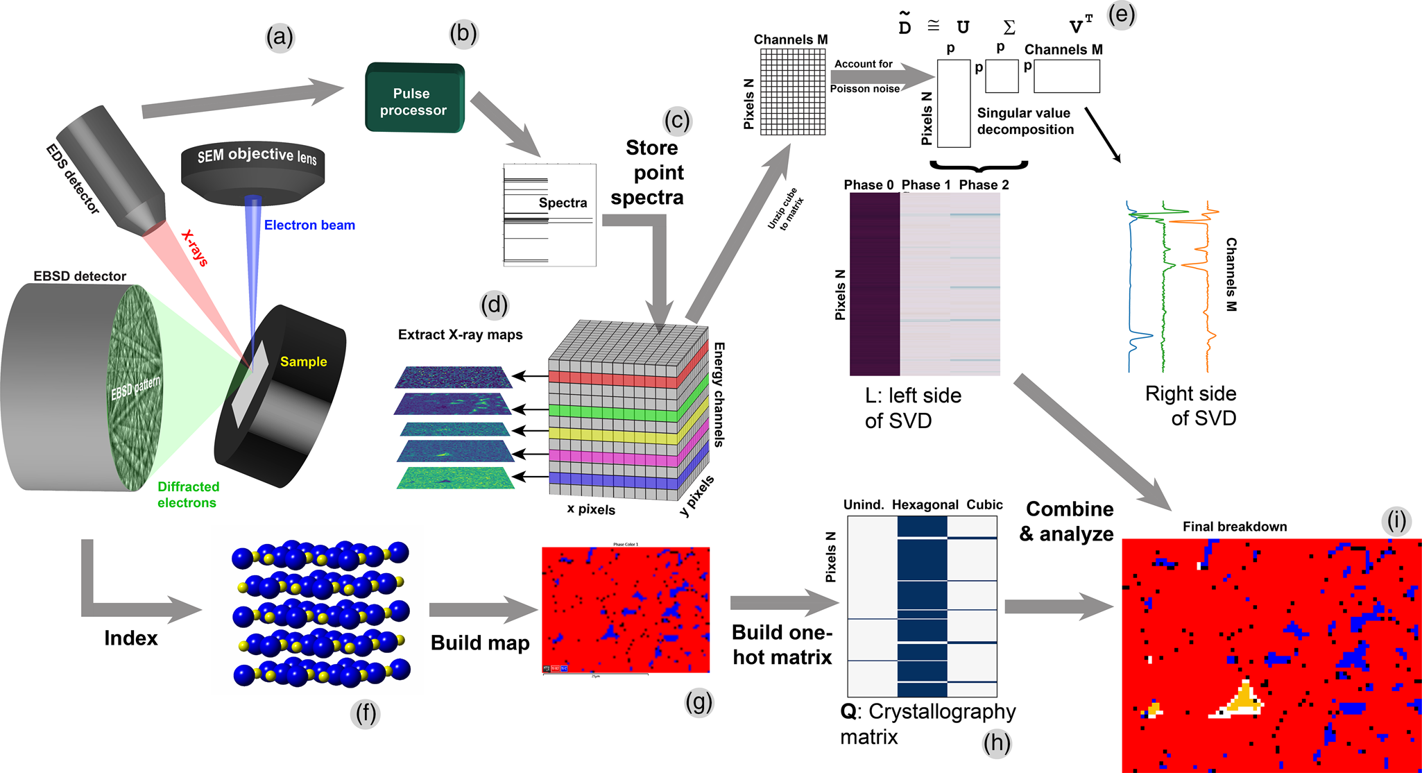
Fig. 1. Schematic of EDS + EBSD acquisition and analysis. (a) The EDS and EBSD data are acquired. (b) EDS pulses are converted and (c) stored into a datacube. (d) The traditional X-ray mapping functionality is extracted from this data. (e) The datacube is unfolded into a matrix and analyzed by singular value decomposition. (f) EBSD patterns are indexed to (g) build a phase map. This phase map is unfolded into a matrix and, when combined with the SVD information, can yield a combined chemical + crystallographic map (i).
To analyze this datacube, the methods refined by Keenan et al. are used (Kotula et al., Reference Kotula, Keenan and Michael2003; Keenan, Reference Keenan, Grahn and Geladi2007; Smentkowski et al., Reference Smentkowski, Ostrowski and Keenan2009). The XSI datacube is unfolded into a matrix D of size N × M and then analyzed [Fig. 1(e)]. Singular value decomposition (SVD) and its close cousin, principal component analysis (PCA), are methods of rank reduction and form the underlying mathematical framework to much of data science, and in the present context, form the backbone of data analytics methods used to analyze the matrix D of the XSIs.
Simultaneously to recording the XSI, the EBSD patterns are analyzed to find the crystal structure [Fig. 1(f)]. The array of EBSD pixels is combined into the phase map [Fig. 1(g)].
To perform SVD of X-ray SIs, it is important to use the insight of Keenan and Kotula (Kotula et al., Reference Kotula, Keenan and Michael2003; Keenan et al., Reference Keenan and Kotula2004a, Reference Keenan and Kotula2004b), specifically that the count data D must be scaled to account for Poisson noise; this is because the noise between X-ray peaks and background are very different (heteroscedastic) and confound algorithms that assume uniform noise (homoscedastic). This is accomplished as described by Keenan and Kotula, specifically that the data matrix D is converted to scaled data  $\hat{{\bf D}}$ via:
 $$\tilde{{\bf D}} = {\bf {GDH}}$$
This  $\tilde{{\bf D}}$ is the “Poisson-scaled data matrix.” As explained elsewhere (Keenan, Reference Keenan, Grahn and Geladi2007), G is a matrix of size N × N with the inverse square root of the mean image of D on the diagonal, and H is a matrix of size M × M with the inverse square root of the mean spectrum of D on the diagonal. This has the effect of making
  $\tilde{{\bf D}}$ very nearly homoscedastic, and therefore more amenable to analysis by SVD or PCA. Once scaled, the SVD is:
 $$\tilde{{\bf D}}{\rm \;} = {\bf U\Sigma }{\bf V}^{\rm T}$$
The columns of U are the left singular vectors, the columns of V are the right singular vectors, superscript T denotes matrix transpose, and the diagonal of Σ carries the singular values. Importantly to the present discussion: (1) the columns of V are the chemical endmembers, and (2) the columns of U are, once refolded, the abundance maps associated with the chemical endmembers. The values of Σ are the relative strengths associated with each component. SVD requires that any two columns of U be mutually orthonormal, and similarly for columns of V, and the singular values are sorted in descending order. As described elsewhere (Kotula et al., Reference Kotula, Keenan and Michael2003; Burke et al., Reference Burke, Watanabe, Williams and Hyde2006; Watanabe et al., Reference Watanabe, Okunishi and Ishizuka2009; Parish, Reference Parish2011), a “scree plot” of eigenvalues (singular values squared) can be plotted, and a knee or slope-break in the plot used to find the number of components to retain. Inverse transformation by G−1 and H−1 return the abundance maps and endmembers into real space from Poisson-scaled space (Keenan & Kotula, Reference Keenan and Kotula2004a, Reference Keenan and Kotula2004b), and post-processing tools such as varimax rotations (Keenan, Reference Keenan2005, Reference Keenan2009; Smentkowski et al., Reference Smentkowski, Ostrowski and Keenan2009) or independent component analysis (Hyvarinen, Reference Hyvarinen1999; Windig & Keenan, Reference Windig and Keenan2015) are commonly applied to find more interpretable results.
Stork & Keenan (Reference Stork and Keenan2010) and Keenan (Reference Keenan, Grahn and Geladi2007) pointed out some disadvantages of the above-described matrix-decomposition methods. First, SVD and its ilk suffer a “parsimony restriction,” in the terminology of Stork and Keenan. This means that the rank of the model cannot exceed the chemical rank of the sample. For instance, if only two chemical elements Fe and Cr are present, then the SVD model will have rank-2. However, if the material consists of, for example, elemental regions of Fe and Cr and an intermetallic compound FeCr, the rank-2-constrained SVD model cannot describe this three-region sample with a rank-3 model. This means that the FeCr region will be described by, for example, the Fe and Cr endmembers with roughly 50–50 abundances in the region of the compound. This requires the analyst to interpret this 50–50 mixture correctly, and the analyst will not be presented with a clear FeCr endmember. The second issue with these methods is that “crisp” phase maps might not be achieved. PCA with varimax rotation to spatial simplicity (VRSS; Keenan Reference Keenan2009), ICA, etc., will provide realistic-looking endmembers, but give negative values in abundance maps (necessarily: if the average of a region's abundance map is to be zero, and there is noise, then some of the pixels must be <0). MCR-ALS (multivariate curve resolution-alternating least squares; Smentkowski et al., Reference Smentkowski, Ostrowski and Keenan2009) under non-negativity constraints, NNMF (non-negative matrix factorization), etc., can remove negative counts, but in turn result in errors in the endmember reconstructions, such as non-physical dips below the Bremsstrahlung in an endmember at the energy locations of peaks strongly present in other endmembers (e.g., Keenan Reference Keenan2009). Other methods, such as NFIND-R (Winter, Reference Winter1999), are also in the early stages of exploration to apply to EDS.
It was the innovation of Stork & Keenan (Reference Stork and Keenan2010), then, to suggest cluster analysis of EDS-SI data. K-means clustering is the classical example (Jain, Reference Jain2010). In K-means, individual objects (pixels in an SI) are clustered based on their similarity; in this case, the similarity of their point spectra. An a priori number of clusters, K, is assigned by the analyst. K-means has the advantage that the cluster centers, which are the spectral endmembers, are very physical in appearance, without artifacts such as non-physical dips below the Bremsstrahlung. Furthermore, because the clusters need not be linearly independent, the parsimony restriction is lifted (Stork & Keenan, Reference Stork and Keenan2010). Highly efficient K-means packages are readily available (e.g., Python's scikit-learn.cluster; Pedregosa et al. Reference Pedregosa, Varoquaux, Gramfort, Michel, Thirion, Grisel, Blondel, Prettenhofer, Weiss and Dubourg2011). However, K-means provides a hard assignment to individual pixels: a pixel is either in one cluster or another. Stork and Keenan suggested applying fuzzy C-means clustering (FCM), in which each pixel's assignment sums to 1.0, and a pixel can be shared among multiple clusters. This is vital, e.g., to describe mixed pixels at a phase boundary. Efficient and easy-to-use fuzzy C-means algorithms are available in Python as scikit-fuzzy (Warner et al., Reference Warner, Sexauer, Unnikrishnan, Castelão, Pontes, Uelwer, Batista, Van den Broeck, Song, Martínez Pérez, Power, Mishra, Trullols and Hörteborn2021).
Most importantly, Stork and Keenan found that clustering on the reduced left-side L of the Poisson-scaled SVD, where L = UΣ from SVD of data  $\tilde{{\bf D}}$ such that
  $\tilde{{\bf D}}{\rm \;} = {\bf U\Sigma }{\bf V}^{\rm T}$, is computationally very efficient. I illustrate this schematically in Figure 1e, which shows the unzipped matrix of spatial abundances (each row is a single pixel) and the spectral endmembers, for a rank p =3 model. Furthermore, the final abundances’ cluster centers (endmembers) are easily recovered from the reduced centers by premultiplication. The net result is to perform clustering on the small N × p matrix L instead of the large N × M matrix
  $\tilde{{\bf D}}$. Because p << M, this saves significant computational time. Clustering on the SVD reconstruction instead of the raw data also allows much improved analysis, because of SVD's noise filtering effects. Overall, the paper of Stork &Keenan (Reference Stork and Keenan2010) should be read carefully for the details.
Application to EBSD
With those foundations laid, let's now discuss what is new in this paper. Specifically, let's define the hypothesis I will test:
-
Hypothesis: Combining EDS and EBSD information into a single matrix will allow efficient cluster analysis to separate crystallographically indistinguishable but chemically distinct phases.
I will take this one part at a time. First, scanning electron microscopy (SEM)-EDS by itself is known to be nicely amenable to cluster analysis, as discussed above in section “Data analytics in X-ray spectrum imaging,” specifically by clustering on the reduced-rank SVD left-hand-side L.
The next—and more difficult—question is how to merge EDS and EBSD data into a format amenable to cluster analysis. Each pixel contains a spectrum of EDS data, but each pixel can contain one and only one crystallographic assignment. Therefore, I need a representation that can easily accommodate each pixel but multiple different crystallographic assignments. An initial thought might be to use an N × 1 single-column matrix and assign each element in the matrix an integer value: 0 for unindexed, 1 for hexagonal, 2 for cubic, etc. However, cluster analysis can be sensitive to the absolute magnitude of different attributes (columns) of the matrix to be clustered. Which is to say, if a large number of crystals were present (10, perhaps), the clustering might give more “weight” to that column and less to the chemically derived columns of L.
To test my hypothesis, I therefore created a “one hot” matrix (Géron, Reference Géron2019), so-called because each pixel has only a single non-zero (“hot”) value. Specifically, I created a matrix, call it Q, where in its zeroth column, a “1” is assigned to each row (pixel) if the pixel is unindexed by EBSD; assigned a “1” in the first column of the pixel is indexed as hexagonal by EBSD; and assigned a “1” in the second column if the pixel is indexed as cubic (Fig. 1h). I use the convention that the first row, column, etc., is “zeroth” and counts up from zero, to be consistent with Python's array indexing. So, for N pixels and z number of crystallographic phases (in which the inevitable “unindexed” pixels are considered a distinct phase), Q is of size N × Z. Because L is of size N × p, then, a combined matrix Y of size N × (p + z) can be constructed as Y = [LN×pQN×z]; this concatenation is easily accomplished in Python via numpy.hstack. To account for the difference in absolute magnitudes of the values between L and Q, I divide L by the absolute value of the largest magnitude element in the matrix L, which reduces the maximum value of L to either +1 or −1, nicely matched to the one-hot values of exactly 1 in the matrix Q. To maintain the same model, V should then be multiplied by this same constant value. This yields, essentially, an arbitrary orthogonal factor model LR where R is this multiplied and then transposed V. My hypothesis, then, is that this combined matrix can be analyzed via clustering to provide a final chemistry and crystallography result that will differentiate chemically distinct but crystallographically indistinguishable phases (Fig. 1i).
In this paper, I will use example data of EDS + EBSD from a complex ceramic with crystallographically ambiguous phases to test this hypothesis.
Materials and Methods
Experimental
The material used was a TiB2 ultra-high temperature ceramic, provided by the Missouri University of Science and Technology. The sample was prepared as described elsewhere (Bhattacharya et al., Reference Bhattacharya, Parish, Koyanagi, Petrie, King, Hilmas, Fahrenholtz, Zinkle and Katoh2019). A small (several millimeters) piece was cut and polished to a mirror finish, with a final polishing step of 50 nm colloidal silica. This provided excellent EBSD patterns.
Simultaneous EDS and EBSD were acquired on a Tescan MIRA3 GMH field-emission SEM equipped with Oxford Instruments Symmetry CMOS-based EBSD detector and Oxford Instruments Ultim Max 170 mm2 silicon-drift detector EDS. Data was acquired using Oxford Instruments AZtec 4.0 software. Data was acquired at 20 keV, 70° tilt, and ≈1 nA probe current. An 80 × 60 pixel, 40 × 30 μm map (500 nm pixel pitch) was acquired. EBSD indexing was performed using TiB2, space group 191 P6/mmm, and TiC, space group 225  $Fm\bar{3}m$, crystal cards. Importantly, TiO, TiC, TiN, and their alloy Ti(CNO) are entirely isostructural (with a rocksalt crystal structure) and indistinguishable crystallographically. The EDS data was exported in the Oxford .RAW (binary) / .RPL (text header) format, and the EBSD data exported in the Oxford .CTF (text) format.
In Figure 2, I show the EDS X-ray maps, EBSD phase and band contrast maps, and the forward-scattered electron image of the general region. X-ray maps are integrated net intensity windows whose full width is the estimated detector resolution at the energy E of the marked line, calculated by shifting 130 eV approximate resolution at Mn Kα (5,893 eV) via Width(E) = [2.5(E-5,893) + (1302)]1/2 (Goldstein et al., Reference Goldstein, Newbury, Echlin, Joy, Romig, Lyman, Fiori and Lifshin1992).

Fig. 2. X-ray maps for Ti, Zr, Si, Al, O, C, and B. The EBSD maps for phases (Hex. = hexagonal) and band contrast. The bottom image is the forward-scatter image, with the map region marked. All figures have the same scale.
Analysis
Anaconda Python 3 was used for all calculations. First, a custom script was used to read the EDS data from the .RAW/.RPL into memory, in which the X-ray point spectra and associated metadata were stored into numerical arrays. The CTF file containing the EBSD results listed each pixel's phase as “0” (unindexed), “1” (TiB2 hexagonal), or “2” (TiC cubic). This was read into memory and converted into a NumPy array. This NumPy array was also converted into a “one-hot” matrix using Scikit-learn's OneHotEncoder. The OneHotEncoder produced a SciPy sparse matrix, and I then used its todense() method to convert the matrix from a sparse SciPy array to a dense NumPy array. This array's size was 4,800 × 3, for 4,800 pixels and 3 phases.
The EDS data was trimmed to −0.2 to 5.79 keV (the Oxford electronics giving some empty channels at negative energies), converted from a dense NumPy array into a compressed sparse column SciPy array, and then scaled for Poisson noise as described above. Because of the high beam current and long pixel dwell time needed for EBSD, the EDS signal was strong and binning was not needed to extract meaningful singular values. SVD was performed on the Poisson-scaled sparse matrix using Python: scipy.sparse.linalg.svds (Virtanen et al., Reference Virtanen, Gommers, Oliphant, Haberland, Reddy, Cournapeau, Burovski, Peterson, Weckesser and Bright2020). The SVD yields the triplet  $\hat{{\bf D}}{\rm \;} = {\bf U\Sigma }{\bf V}^{\rm T}$, and I then define
  ${\bf L} = {\bf U\Sigma }$. Recall that L is size N × p, where N is the number of pixels (80 × 60 = 4,800) and p is the rank of the SVD, which is this case is p = 3.
Results and Discussion
EBSD finds two crystallographic phases, but EDS finds three chemical phases. This is, of course, the crux of the problem I wish to address. The phase map in Figure 2 labels these two crystallographic phases as “Hex.” (Hexagonal, red) and “Cubic” (blue). Unindexed pixels, essentially a third null phase, are black.
The PCA analysis, Figure 3, is the result of returning the noise-scaled SVD analysis from the Poisson-scaled space back to the original real space, and then re-orthogonalizing using Keenan's “fPCA” method (Keenan, Reference Keenan, Grahn and Geladi2007). The first component (Fig. 3, top row) is the mean spectrum and mean image. The second component (Fig. 3, middle row) shows the differences between the matrix and the precipitates. The Ti and B peaks are negative in that endmember, which indicates the precipitates are weak in these elements. These negative “counts” are indicative of the problem with simple SVD/PCA analyses: their difficult interpretability. The third component (Fig. 3, bottom row) shows the differences between the two precipitate populations.

Fig. 3. PCA of the XSI, returned from noise-scaled space to real space and re-orthogonalized. The first component (top row) describes the mean (primarily Ti-Zr-Al-O-B). The second component describes the differences between the matrix and the precipitates. The third component (bottom row) describes the differences between the precipitates. Spectral endmembers are scaled to an integral of 1.0.
A more interpretable approach is seen in Figure 4, which is the “varimax rotation to spatial simplicty” (VRSS) (Keenan, Reference Keenan2009) analysis. This shows that there are three distinct regions, specifically, TiB2 matrix (top row); (Ti,Zr,Al,O,(Ca?))-oxide precipitates (middle row); and Ti(C,N,O) precipitates (bottom row). Other methods, such as varimax-rotated PCA, NNMF, and NFIND-R, are certainly possible and give substantially similar results, but VRSS provides a clear interpretation of the X-ray data here.

Fig. 4. Varimax rotation to spatial simplicity analysis of the XSI. Three independent components are found: Ti-B (top); (Ti,Zr,Al,O,(Ca?)) (middle); Ti-(C,N,O) (bottom). Spectral endmembers are scaled to an integral of 1.0. The arrow indicates a precipitate of interest in later analysis.
From this starting point, I begin the specific analysis of the data to explore the use of combined elemental and crystallographic information via clustering.
First is K-means and fuzzy C-means analysis of the EDS data. K-means cluster analysis of the left-side of the SVD, L, is shown in Figure 5 and fuzzy C-means in Figure 6. These use the methodology described for fuzzy C-means described by Stork & Keenan (Reference Stork and Keenan2010). K-means was calculated using scikit-learn (Pedregosa et al., Reference Pedregosa, Varoquaux, Gramfort, Michel, Thirion, Grisel, Blondel, Prettenhofer, Weiss and Dubourg2011) and fuzzy C-means using scikit-fuzzy (Warner et al. Reference Warner, Sexauer, Unnikrishnan, Castelão, Pontes, Uelwer, Batista, Van den Broeck, Song, Martínez Pérez, Power, Mishra, Trullols and Hörteborn2021). From this starting point, I begin the specific analysis of the data to explore the use of combined elemental and crystallographic information via clustering. For both cluster analyses, I found that four clusters provided the most insightful analysis. With three clusters, the result replicates the VRSS results. With four clusters, an additional component not found in the VRSS result is discovered, providing new insight. However, five clusters resulted in non-physical checkerboarding in which the matrix (TiB2 phase) was split into two different clusters without any physical meaning.

Fig. 5. K-means clustering analysis on the SVD-reduced EDS data. Four clusters (phases) describe the data very well. Spectral endmembers are arbitrarily scaled and offset vertically for visibility.

Fig. 6. Fuzzy C-means clustering of the SVD-reduced EDS data. Four clusters (phases) describe the data very well. Spectral endmembers are arbitrarily scaled.
The reason that four clusters, instead of three, appears more insightful can be explained by looking at the precipitate that is arrowed in Figures 4–6. In either cluster analysis figure, the “oxide 1” spectral endmember shows more B-K X-ray intensity and less O-K X-ray intensity than “oxide 2”; oxide 1 looks like a linear combination of the matrix and oxide 2, and this point will come back later. In the VRSS analysis (Fig. 4), the same particle shows weaker “oxide” contribution than the large oxide particle, and more contribution from the matrix phase. This is likely interpretable as the arrowed particle being very thin, and the 20 kV electron beam exciting noticeable amounts of B, and noticeably less O, at those points. This illustrates nicely Stork and Keenan's point that cluster analysis does not suffer the “parsimony restriction” that factor analysis methods suffer (Stork & Keenan, Reference Stork and Keenan2010).
So, now, the next question is, how can the chemical (EDS) and crystallographic (EBSD) information be combined into a single comprehensive analytical look at the sample? As noted above in section “Application to EBSD,” I hypothesize that a cluster analysis applied to a combined matrix of chemical information and crystallographic information will provide the desired differentiation of crystallographically indistinguishable but chemically distinct phases.
At first, I can combine the SVD left-side L (scaled to a maximum absolute value of 1.0) and a matrix Q of the crystallographic identifications into a single matrix Y. This is illustrated in Figure 7. Then, K-means clustering of this matrix Y is performed. K-means clustering, as in Figure 5, produces a phase assignment map and spectral endmembers. The cluster centers of a K = 5 analysis of the matrix in Figure 7 is given in Figure 8a. Figure 8a shows the cluster centers directly derived from clustering Figure 7. Figure 8b shows the cluster assignment map. Although Stork & Keenan (Reference Stork and Keenan2010) give an equation that allows the recovery of the (Poisson-space) endmembers, P, from the SVD's right-side endmembers, Vk and the cluster centers  $\hat{{\bf P}}$, such that
  ${\bf P} = {\bf V}_k\hat{{\bf P}}$, and which can be returned to real-space by dividing by the spectral Poisson-scaling vector H, here I found the simply summing the point spectra under each cluster map provides an identical result (±numerical rounding after normalization to highest peaks), and use the summed spectra under each cluster assignment map, scaled to the number of pixels per phase as that endmember (i.e., cluster centers). It is important to note that the final three columns of the cluster centers are the crystallographic assignments and should be truncated before applying that equation. The final cluster centers, in real (spectral) space, are given in Figure 8c and a detailed view of the low energy lines in Figure 8d.

Fig. 7. Illustration of unzipping L and Q into a combined matrix Y for analysis. Note that L is scaled to a maximum absolute value of 1.0.

Fig. 8. (a) Cluster centers found by K = 5 K-means of the matrix in Figure 7. (b) The associated cluster assignment map. (c) The cluster centers after conversion from the reduced SVD space to real space. (d) A detailed view of the low-energy X-ray lines.
Figures 8c and 8d show the insight gained from the proposed method. Cluster #0 (red) is the matrix and shows Ti and B lines clearly and was assigned to the hexagonal phase. So far, so good: this is the TiB2 matrix. Cluster #1 (blue) shows Ti and C and a cubic assignment. This, also, makes sense given the X-ray maps and EBSD maps in Figure 2; this is a carbon-rich Ti(C,N,O) alloy and will be called TiC for simplicity. Cluster #2 (black) is chemically indistinguishable from the matrix but is “unindexed” phase assignment; these are matrix pixels with bad EBSD patterns, mostly from grain boundaries that gave overlapped Kikuchi bands. This phase could have been eliminated by cleaning the EBSD results (Brewer & Michael, Reference Brewer and Michael2010) but I decided not to apply EBSD data cleaning on my data.
It is for Cluster #3 (gold) where the benefit of this new technique becomes apparent. The EBSD map in Figure 2 showed the triangular particle on the left-center of the map as cubic, and indistinguishable from the carbides of Cluster #2. However, here, the chemistry seen in the spectral endmember is entirely different—Al,Zr,Ti,O(,Ca)—compared to the TiC chemistry of Cluster #2 and despite the cubic phase assignment that, by EBSD alone, was indistinguishable from the TiC. Thus, the hypothesis in section “Application to EBSD” is confirmed: combined EDS + EBSD via cluster analysis has indeed differentiated chemically distinct but crystallographically ambiguous phases. Had I indexed with K = 4, this would be a satisfying end to the analysis. However, the K = 5 clustering shows the fifth cluster, Cluster #4 (gray), which is very surprising indeed. The Al and Zr lines are intermediate between the Al,Zr,Ti,O(,Ca) (gold) and TiB2 (red) phases, as is the B line. The phase assignment is, surprisingly, hexagonal. This phase, then, appears to identify TiB2 (hexagonal) pixels in which the blooming of the electron beam underneath the surface excited X-rays from a region larger than the small surface area sampled by EBSD. Cluster #4 (gray), then, describes the different spatial resolutions between the EDS and EBSD signals. Indeed, a Monte Carlo simulation using CASINO (Hovington et al., Reference Hovington, Drouin and Gauvin1997) shows ~1,000 nm beam broadening of a 20 keV beam at 70° tilt onto TiB2 of 4.5 g/cm3; compares this roughly 1,000 nm to the 500 nm step size of the experiment and the very small (<10 nm) size of the actual field emission probe at a modest beam current of ≈1 nA. Although EBSD spatial resolution is difficult to estimate, it will be closer to the probe size than the interaction volume; based on measurements on other materials (Chen et al., Reference Chen, Kuo and Wu2011), around 100 nm seems a reasonable guess here.
It is a well-known limitation of clustering methods that if different features being clustered on very different scales, the results of the cluster analysis can be skewed; therefore, I will try the same analysis, but instead of using L (where L = UΣ), what if only U is used as the basis for the clustering? In this analysis, the trace of Σ is [1,200.0, 118.2, 71.5]. Which is to say, the 0th column of L is about 10× stronger than the 1st column, which is about twice as strong as the 2nd column. U, conversely, is orthonormal (each column is a unit vector), so the scales are much closer. Figure 9a shows this matrix; a comparison of Figure 9a to Figure 7 shows that the absolute values of the elements in columns 0, 1, and 2 are much closer. It is therefore reasonable to assume the clustering behavior will be more sensitive to smaller features. The actual cluster centers in Figure 9b are not appreciably different from those in Figure 8a—note that the order in which clusters are assigned is arbitrary. It is, in Figure 9c, the cluster assignment map, where this U-based analysis begins to differ from the L-based analysis. The assignment is a bit noisier; speckle is observed, which was absent from the L-based cluster assignment map, Figure 8b. The Al,Zr,Ti,O(,Ca) cubic phase (gold), the TiB2 hexagonal matrix phase (red), and the unindexed TiB2 phase (black) are unchanged. Careful inspection of the carbide cubic phase (blue) finds little or no difference between the L-based and U-based assignment, but large differences appear in the chemically mixed hexagonal phase (gray). First, gray edging is seen around the carbides in the U-based which was not observed in the L-based. These seem to indicate that the threshold to assign the phase's chemistry to the gray phase is lower in the U-based assignment. This makes sense because the scale difference between the phases was removed and smaller effects in the non-matrix should be visible. More interesting, additional entire regions, such as the gray particle marked by the white arrow in Figure 9c, are discovered. Careful inspection of the X-ray maps (Fig. 2) indicates that, indeed, a very weak O and C signal is seen at that location. Given the hexagonal indexing and lack of visible boundary at that site in the band contrast map, this may be a shallowly buried oxycarbide excited by the penetrative 20 kV beam.

Fig. 9. (a) U-based construction of the chemistry + crystallography matrix Q. (b) Cluster centers obtained by K = 5 K-means of the matrix in (a). (c) Cluster assignment map. (d) Chemistry endmembers + phase assignments derived from (b).
Ultimately, the comparison between the U-based (Fig. 9) and L-based (Fig. 8) analyses appears to be that the U-based is more sensitive to both noise and small signals, so the choice of one over the other might involve a decision toward sensitivity versus map crispness; for these maps, the K-means computation times were <5 s, so analyzing in both methods and comparing them are resource-light and thorough.
For one last comparison, the fuzzy C-means results (Fig. 6) were converted into an L-like matrix, where if a pixel was >0.8 in a single cluster, it was assigned 100% to that pixel, and the same clustering performed. Initial results were grossly incorrect, in that with K = 5, the TiC and Al,Zr,Ti,O(,Ca) cubic phases were assigned to the same cluster. However, if analyzed with K = 6, this FCM-based analysis provides a very similar result to the U-based analysis, Figure 10. The TiB2 (red), Al,Ti,Zr,O(,Ca) (gold), and TiC (blue) phases are unchanged. The hexagonal edging-effect phase (gray) is seen again, including at the “buried” feature seen in Figure 9c arrowed, but a sixth assignment, very similar to the gray assignment, green in Figure 10, shows a second edge-effect hexagonal phase with perhaps very slightly less of an O-line than the gray edge-effect phase. In other words, this provides perhaps the cleanest look yet—the buried phase is found like in the U-based but with less speckle—although at the cost of slightly more complicated interpretation, owing to the sixth phase.

Fig. 10. Cluster assignment maps and cluster-center endmembers + crystallographic assignments for the FCM-based analysis. The “cubic” phases are TiC (blue) and (Al, Zr, Ti, O) (gold). The hexagonal phases are TiB2 (red), Ti-B-O (Green), and Al-Zr-Ti-B mixed (gray).
Conclusions
The proposed cluster analysis method reliably and effectively differentiated the two cubic phases, TiC and Al,Zr,Ti,O(,Ca), in this tested sample. Different methods already exist to differentiate phases in EBSD that cannot be differentiated by the simple Hough-based methods. For instance, dynamical pattern simulation followed by dictionary comparison (Chen et al., Reference Chen, Park, Wei, Newstadt, Jackson, Simmons, De Graef and Hero2015) provides very high fidelity in indexing, but is computationally expensive and has significant start-up effort involved. Detector vendors have vendor-specific methods for merging the EBSD and EDS data to find the different phases. However, these methods can involve a certain amount of black-box software and are also not transferrable from one vendor's system to another.
The proposed method has several advantages:
1. The proposed method successfully differentiates chemically different phases that had indexed identically using the on-microscope Hough-based approach.
2. The proposed method is computationally cheap; for the 80 × 60 pixel dataset here, the full analysis is in the order of minutes, and the majority of that time is spent on the FCM clustering (Fig. 6), because the FCM is repeated 512 times to help ensure convergence to an optimum solution from the random initializers.
3. This method is vendor agnostic, and only requires that the EBSD phase assignments and the EDS pixel spectra be readable and tagged to the pixels.
4. This method is provided in the Supplementary material, section 6, as open-source software and is freely available.
The primary disadvantages to the present technique are the following:
1. The choice of the number of clusters to determine requires a combination of domain knowledge and trial and error; however, the vendor-specific methods share this drawback.
2. Vendor-specific methods can be performed using the on-microscope software and do not require any programming knowledge.
3. The choice of L-based, U-based, or FCM-based starting matrix provides somewhat different results; however, the major phase assignments are unchanged, and only the very small differences (such as tiny contributions of Al-Zr to the matrix spectral component) are different.
Regardless, it seems that this method has potential as a machine-learning approach to the differentiation of crystallographically ambiguous phases via combined EDS + EBSD. Further development is promising as a simple and effective way to identify such phases.
Acknowledgments
The author thanks to Dr. Hanns Gietl and Dr. John Echols, ORNL, for critiquing the manuscript. This manuscript has been authored by UT-Battelle, LLC under Contract No. DE-AC05-00OR22725 with the U.S. Department of Energy. The United States Government retains and the publisher, by accepting the article for publication, acknowledges that the United States Government retains a non-exclusive, paid-up, irrevocable, worldwide license to publish or reproduce the published form of this manuscript, or allow others to do so, for United States Government purposes. The Department of Energy will provide public access to these results of federally sponsored research in accordance with the DOE Public Access Plan (http://energy.gov/downloads/doe-public-access-plan). Sample courtesy G. Hilmas & W. Fahrenholtz, Missouri University of Science and Technology.
Financial support
This work was supported by US Department of Energy, Office of Science, Fusion Energy Sciences, under contract number DE-AC05-00OR22725.


 Open access