


Introduction
Growth and size represent two of an animal's most important traits (Haldane Reference Haldane1926). Notably, growth provides the framework for an animal's life history (Alonzo and Kindsvater Reference Alonzo, Kindsvater, Jørgensen and Fath2008). The study of growth in extinct organisms, particularly in early animals, can help to answer important questions in evolutionary developmental biology, including how developmental processes evolve (e.g., Hughes et al. Reference Hughes, Hong, Hou and Fusco2017). However, growth in such organisms cannot be studied directly in the field or aquaria. As a result, paleontological studies of “growth” are often based on relative age data (e.g., in trilobites; Fusco et al. Reference Fusco, Garland, Hunt and Hughes2012; Hughes et al. Reference Hughes, Hong, Hou and Fusco2017). Here, we distinguish between the absolute and relative age an animal can have. In some taxa, absolute age can be readily estimated precisely; for example, by counting daily rings in the otoliths of teleost larvae (Jones Reference Jones1986) or the statoliths of squid larvae (Pauly Reference Pauly, Payne, Lipinski, Clarke and Roeleveld1998b). When absolute ages cannot be estimated, for example, when analyzing length–frequency (L/F) data, ages are relative, that is, added to an assumed age at some small arbitrary length.
Outside paleontology, “growth” is understood to link an animal's size (length or weight) with time elapsed during its ontogeny (absolute age). Thus, an increase in the maximum size of the species in a clade of water-breathing ectotherms (WBEs) over evolutionary time is not “growth” in this restricted sense, and neither is the identification of successive anatomical stages such as molt instars. On the other hand, assuming that the successive peaks in a length distribution represent annual cohorts (or year classes) is an inference about growth. As a result, any instance in the fossil record where growth can be inferred based on absolute age is of high importance, as it allows direct comparison with models of growth in extant taxa. Such comparative analyses are key to the emerging discipline of paleo-evo-devo (Minelli and Fusco Reference Minelli and Fusco2008). Even a small number of instances where such analysis can be conducted is useful, as the relationship between absolute and relative growth in these examples can then be used to make inferences about other fossil taxa.
Trilobites provide some of our best insights into growth in early animals and are one of the most diverse groups in the fossil record (Paterson Reference Paterson2020). As noted earlier, studies of trilobite growth have generally been based on measures of relative growth and, in particular, patterns of change in relation to the molt cycle. These usually focus on differences in size and shape between specimens (e.g., Hong et al. Reference Hong, Hughes and Sheets2014; Holmes et al. Reference Holmes, Paterson and García-Bellido2020) or in relation to changing morphologies between successive molt instars (e.g., Fusco et al. Reference Fusco, Hong and Hughes2014, Reference Fusco, Hong and Hughes2016; Dai et al. Reference Dai, Hughes, Zhang and Fusco2021; Holmes et al. Reference Holmes, Paterson and García-Bellido2021a; Hughes et al. Reference Hughes, Adrain, Holmes, Hong, Hopkins, Hou, Minelli, Park, Paterson, Peng, Webster, Zhang, Zhang and Fusco2021). Even in life, trilobites, like other arthropods, lacked accretive hard parts that allow their age and growth to be determined directly, as in some other WBEs like fish and mollusks (Pannella and MacClintock Reference Pannella and MacClintock1968; Jones Reference Jones1986; Jones and Quitmyer Reference Jones and Quitmyer1996; Pauly Reference Pauly, Payne, Lipinski, Clarke and Roeleveld1998b). One potential example of absolute growth in trilobites is the results of Cisne (Reference Cisne1973), who presented L/F data on the Late Ordovician trilobite Triarthrus eatoni Hall, Reference Hall1838 with pronounced size-distribution peaks that he interpreted as annual cohorts. Here, we apply methods developed within fisheries science and marine biology (for studying the growth of fish and invertebrates lacking annual or other skeletal marking) to reanalyze the data presented by Cisne (Reference Cisne1973), in order to provide estimates of absolute growth and mortality parameters. For comparison, a similar analysis was also performed on a modern analogue, the marine isopod Ceratoserolis trilobitoides (Eights, Reference Eights1833).
Application of Growth Models to Trilobites
The absolute ages of T. eatoni specimens estimated by Cisne (Reference Cisne1973) assumed a linear model of growth in length with time. However, we know from extant WBEs (and other metazoans) that growth is generally asymptotic, with the growth rate declining with time. Indirect support for this in trilobites comes from the presence of encrusting epibionts on large holaspides of the phacopid Flexicalymene, which has been used to suggest increasing time between instances of molting (representing relatively constant size increases due to Dyar's rule; see Fusco et al. Reference Fusco, Garland, Hunt and Hughes2012), and thus a decline in absolute growth (Brandt Reference Brandt1996). In extant WBEs (including arthropods), this decline is well described by an asymptotic growth curve such as the von Bertalanffy growth function (VBGF), and this is the model adopted here. Given the nature of the fossils at hand, the approach used here must rely on the analysis of L/F data. Moreover, the growth model or equation used to fit the available L/F data analysis must be selected a priori, as the available L/F data do not allow for contrasting the performance of different growth models (see “On the Potential Suitability of Different Mathematical Models to Describe the Growth of Trilobites” in the Supplementary Material for a discussion of alternative models; see https://doi.org/10.5281/zenodo.6640357).
The growth model chosen here builds on the foundation of Pütter (Reference Pütter1920) and von Bertalanffy (Reference Bertalanffy1938), who viewed growth rate (dw/dt) as the net result of two processes with opposite signs, that is,
 $$\displaystyle{{dw} \over {dt}} = Hw^d\;\ndash kw$$
where the two terms on the right are anabolism and catabolism, respectively, and where d < 1.
As interpreted by Pauly (Reference Pauly2019, Reference Pauly2021), anabolism refers to the synthesis of body tissues. This process requires an amino acid pool to provide building blocks for proteins and ATP to provide the “energy” required for their synthesis. Here, ingested food is not “energy”; rather, food is oxidized (i.e., “burned”) to generate ATP, which may be considered to be “energy” (Cox and Nelson Reference Cox and Nelson2008). Thus, the process of anabolism requires oxygen, which must enter the body through some permeable surface (e.g., in trilobites, the exopod functioned as a gill; Hou et al. Reference Hou, Hughes and Hopkins2021). Therefore, the parameter d in equation (1) is equivalent to the exponent of a relationship linking respiratory surface area (S) to body weight of the form S = a · Wd. Because S is a surface, it cannot keep up with a growing volume (or weight), and hence d is generally 0.6–0.7 in small fishes (Pauly Reference Pauly2019, Reference Pauly2021) and 2/3 in small crustaceans (von Bertalanffy and Krywienczyk Reference Bertalanffy and Krywienczyk1953). Thus, assuming that d was 2/3 in trilobites is a parsimonious hypothesis. In contrast to anabolism, catabolism is directly proportional to body weight, because it consists of the spontaneous denaturation of protein and other molecules contributing to that weight (Brandts Reference Brandts and Rose1967; Goldberg and St. John Reference Goldberg and St John1976; Hawkins Reference Hawkins1991). Spontaneous denaturation, that is, loss of quaternary structure by molecules, occurs throughout the body and requires neither “energy” nor oxygen to be supplied. It is therefore weight proportional, even if denaturation proceeds at different rates in different molecular types.
The integration of equation (1) when assuming d = 2/3 results in the standard VBGF, which implies that asymptotic size is reached when Hwd = kw. The curvilinear VBGFs for length and weight growth resulting from this integration have found wide application in fisheries and marine biology because they describe very well the growth of WBEs, that is, fish and marine invertebrates (see www.fishbase.org and www.sealifebase.org). On the other hand, “linear” growth of WBEs in length and/or weight appears to have never been demonstrated in Recent organisms (see, e.g., Wang et al. Reference Wang, Hunt, Liang, Pauly and Pakhomov2017). Thus, there is no reason to assume that linear growth would have occurred in ancient WBEs such as trilobites. This provides a rationale for reexamining the inferences on growth and related attributes of T. eatoni, notably mortality and longevity estimated by Cisne (Reference Cisne1973), based on his assumption of “linear” growth, with some emphasis on comparison with the growth of crustaceans in general and the benthic marine isopod C. trilobitoides in particular.
Materials and Methods
Triarthrus eatoni Sample of Cisne (Reference Cisne1973)
The data analyzed here are those of Cisne (Reference Cisne1973), based on a sample of the olenid trilobite T. eatoni (Fig. 1) from the base of “Beecher's Trilobite bed,” a ca. 4 cm mudstone turbidite bed present at a locality within the Frankfort Shale, near Rome, New York, U.S.A. (Farrell et al. Reference Farrell, Martin, Hagadorn, Whiteley and Briggs2009, Reference Farrell, Briggs and Gaines2011). Specimens range in size from protaspides (the smallest postembryonic stage, <1 mm long) to large holaspides (adults, up to ca. 40 mm). Pervasive soft-part preservation of non-biomineralized structures such as appendages (e.g., Whittington and Almond Reference Whittington and Almond1987; Hou et al. Reference Hou, Hughes and Hopkins2021) allowed Cisne (Reference Cisne1973) to identify 467 specimens that were alive at the time of burial (from a total of 574), of which 295 were complete enough following preparation to allow sagittal length to be measured. As such, the sample represents one of the most unbiased estimates of a census population known from the trilobite fossil record.
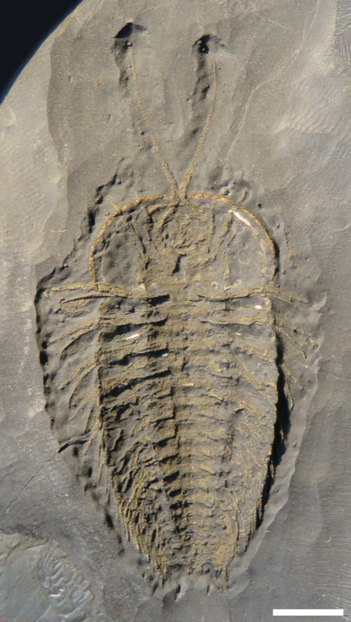
Figure 1. A ventral view of the olenid trilobite Triarthrus eatoni from the Ordovician of New York State (U.S.A.) showing exceptional preservation of appendages. Scale bar, 5 mm. (Natural History Museum, London; photo by J.D.H.)
In his analysis, Cisne (Reference Cisne1973: fig. 2, table 1) recognized several peaks in the population size (length) distribution, which he interpreted as representing annual cohorts. He reported the two largest groupings (his groups II and III) as having mean lengths of ca. 10.2 mm and ca. 19.1 mm. These clearly do not represent molt instars, as this would imply an unrealistic per-molt growth rate (~2) between stages (see Fusco et al. Reference Fusco, Garland, Hunt and Hughes2012). The third peak is much lower than the second, while the fourth and fifth peaks continue a more modest decline. While there appears to be substantial size variation within the cohorts, this is expected, given that individuals grow and molt at different rates (e.g., see the comments by R. G. Hartnoll in Sheldon [Reference Sheldon1988]).
Annual cohorts have not yet been reliably identified in other trilobites, most likely because instances in the fossil record that might accurately preserve census samples of living populations are extremely rare. These invariably rely on a representative sample being captured by a single event (e.g., a sediment gravity flow or turbidite). Even then, there is no way of knowing whether the sample is truly unbiased. For example, it may have been easier for larger specimens to escape the turbidite, and they may be underrepresented in the sample. Likewise, members of different size classes may live in different environments, making them more or less likely to be captured in such an event. However, it should be noted that although such a sample will be biased in terms of reflecting the population structure as a whole, this does not necessarily preclude the identification of certain population characteristics, such as recruitment pulses (if present). Even after such a deposit has been identified, strict sampling procedures are required to maintain the integrity of the sample. These are often not met, particularly with historical collections (Whitaker and Kimmig Reference Whitaker and Kimmig2020). In this case, Cisne (Reference Cisne1973) noted that a number of specimens (~100) were given away to other collections and that these were probably mostly of medium size. However, he considered any bias introduced from this to be minimal (as do we).
There are a number of published examples that have been interpreted as trilobite “census samples.” Paterson et al. (Reference Paterson, Jago, Brock and Gehling2007: fig. 5A) described a sample of the early Cambrian Balcoracania dailyi from the Warragee Member of the Billy Creek Formation that likely represents a largely unbiased sample of a living population. It is noteworthy that this sample has a similar right-skewed distribution to that of the T. eatoni sample analyzed here. However, the scarcity of larger specimens in the B. dailyi sample makes any identification of recruitment cohorts problematic. Brezinksi (Reference Brezinski1986) interpreted a sample of the Ordovician trilobite Ampyxina bellatula as a census population, the distribution of which shows a roughly normal distribution with eight to nine subordinate peaks consistent with his interpretation of molt instars (based on size differences between peaks). However, this sample only contains holaspid (adult) specimens, and thus represents only a part of ontogeny. The peak of the overall distribution itself may represent a recruitment cohort; however, based on the limited size interval, it is difficult to determine whether this is the case. Incidentally, Brezinski (Reference Brezinski1986) apparently made several errors in his analysis, including the interpretation of molt instars as recruitment pulses and confusing relative and absolute growth (see Sheldon Reference Sheldon1988). This highlights the importance of the issues discussed in the present contribution.
Despite the absence of other examples in the fossil record, our assumption that the peaks in the T. eatoni size distribution represent recruitment cohorts is justified, for the following reasons: (1) We have fit Gaussian finite mixture models to a simulated dataset based on the size distribution of Cisne (Reference Cisne1973), and the best-supported models suggest that groups II and III are drawn from separate distributions (Fig. 2; see “Testing for Multiple Distributions”). (2) Specimens can be clearly identified as being alive when buried (or very recently deceased) based on both articulation state and soft-part preservation. This is essentially a “gold standard” for recognizing a census sample and not present in the examples discussed earlier. (3) The collection biases are known, and it is unlikely that these would affect the ability to discern recruitment cohorts. (4) The observed size distances between annual peaks are consistent with modern crustaceans, for example, mean lengths of 29.3, 44.4, 55.8 and 62.9 mm were reported for four annual cohorts of the deep-water shrimp Aristeus antennatus, implying percentage increases of 151%, 126%, and 112% (Ragonese and Bianchini Reference Ragonese and Bianchini1996), compared with 10.2, 19.1, 32.0, and 38.2 mm (187%, 167%, and 119%) for the larger groups in T. eatoni (note the decreasing growth in percentage length in both cases). Likewise, two annual cohorts with peaks of ca. 12 and 40 mm (333%) were observed for juveniles of the crab Ranina ranina (Kirkwood et al. Reference Kirkwood, Brown, Gaddes and Hoyle2005). The size distribution of R. ranina is also very similar to that of T. eatoni, showing a very large younger cohort and a much smaller older one (Kirkwood et al. Reference Kirkwood, Brown, Gaddes and Hoyle2005: fig. 3). Annual peaks identified in the marine isopod Ceratoserolis trilobitoides (represented by the molt classes III and V of Luxmoore [1981]) varied from ca. 15 to 23 mm (153%). These examples suggest that T. eatoni size-distribution peaks are well within the range of annual growth for extant crustaceans. (5) If groups II and III are assumed to be annual cohorts (representing average size increase of 187%), it can be estimated that T. eatoni probably molted (on average) approximately five to seven times during this period. Per-molt growth rates of trilobites were largely constant across ontogeny (consistent with Dyar's rule; e.g., Fusco et al. Reference Fusco, Garland, Hunt and Hughes2012), and trilobites living in environments similar to that of T. eatoni show size increase of ca. 110%–115% per molt (Fusco et al Reference Fusco, Garland, Hunt and Hughes2012; Hou et al. Reference Hou, Hughes, Yang, Lan, Zhang and Dominguez2017; Holmes et al. Reference Holmes, Paterson and García-Bellido2021b; Hopkins Reference Hopkins2021). This is consistent with extant arthropods, for example, decapod crustaceans (e.g., Corgos et al. Reference Corgos, Sampedro, González-Gurriarán and Freire2007). Here, therefore, we proceed with the explicit assumption that Cisne (Reference Cisne1973) was correct in identifying his groups (specifically II and III) as annual cohorts.

Figure 2. Density estimate (line) of the Gaussian finite mixture model fit to the simulated size (length) distribution of the trilobite Triarthrus eatoni (based on data from Cisne [Reference Cisne1973]). Results suggest that the two peaks are drawn from separate distributions.
Testing for Multiple Distributions
Cisne (Reference Cisne1973: table 1) only provided summary statistics for his L/F T. eatoni data. While this and the size distribution (Cisne Reference Cisne1973: fig. 2) provide the input data required for the growth models employed here, the lengths of individual specimens were not provided. However, to test for multiple distributions, we can simulate these data based on information from the published size distribution. We randomly generated the same number of length measurements within each 1 mm size bin of Cisne (Reference Cisne1973: fig. 2) for groups II and III to create a dataset for testing whether the observed data are likely to be drawn from one or more distributions.
Using the function Mclust() from the mclust package (Scrucca et al. Reference Scrucca, Fop, Murphy and Raftery2016), we fit Gaussian finite mixture models to the simulated dataset to test its suspected multidistribution nature. This function tests models with different numbers of components and selects the most likely model based on the Bayesian information criterion. Note that these models assume that the data are drawn from one or more normal distributions. Models were fit to both logged and unlogged data (group II appears to be right skewed, and logging normalizes this somewhat). In both cases, models with three components were the most likely. The models suggest that group II is comprised of two distributions with similar mean values, while group III is a separate distribution. In the simulation we ran, the means of the two group II distributions were 8.78 and 9.88 mm, while the mean of the group III distribution was 19.80 mm (i.e., very similar to the mean estimates of Cisne [1973]). It is likely that the somewhat nonnormal group II distribution is causing the models to suggest that this is composed of two normal distributions rather than one. However, the important point is that group III is clearly identified as a distribution separate from group II. Density estimates were then produced for each data point based on the three-component Gaussian finite mixture model (using the function densityMclust() and plotted for visual confirmation of how the model fits the data; Fig. 2). The R code for this analysis is brief and appended to the Supplementary Material rather than as a separate R script file (see https://doi.org/10.5281/zenodo.6640357).
Growth Models
For length, the VBGF has the form:
 $$L_t = L_\infty \cdot ( 1-e^{{-}K\cdot ( t - t_0)} ) $$
where Lt is the mean length at age t of the WBEs; L is their asymptotic length, that is, the mean length attained by the surviving WBEs after an infinitely long time; K (here: yr−1) expresses how rapidly L ∞ is approached; and t 0 is a parameter that corrects for the fact that the VBGF generally fails to describe the growth of the larval stages of WBEs (Pauly Reference Pauly1998a). When t 0 is assumed to be zero, age becomes “relative age” (t′).
Typically, the parameters of the VBGF are estimated by nonlinear fitting of length-at-age data pairs. However, we cannot use this technique here because—contrary to Cisne's (Reference Cisne1973) assumption—only two of the size groups he identified (II and III in our Fig. 3A) could be reliably assumed to be successive annual groups. However, two alternative methods of estimating the parameters of the VBGF are available. The first is approximate and involves identifying only two size groups (L 1, L 2) separated by a known or assumed time interval (t 2 − t 1).

Figure 3. Aspects of the growth of the olenid trilobite Triarthrus eatoni; A, Length–frequency (L/F) sample assembled by Cisne (Reference Cisne1973), with his assumed annual groups (I to V); B, electronic length frequency analysis (ELEFAN) analysis of the same L/F data, after regrouping them in 3 mm bins and restructuring via a smoothing procedure to identify peaks (black, positive histograms) and troughs (white, negative histograms), which allowed a von Bertalanffy growth function (VBGF) parameter set to be determined that produced a growth curve that hit most peaks and avoided most troughs; C, goodness of fit of a VBGF with L ∞ = 41 mm with over a wide range of K values, identifying K = 0.29 yr−1 as the best estimate; D, the length and likely weight growth curves for T. eatoni.
Given such data, the parameter K of the VBGF can be estimated from:
 $$K\approx [ ( L_2-L_1) /( t_2-t_1) ] /L_\infty $$
where L ∞ is an estimate of the asymptotic length (Gulland and Holt Reference Gulland and Holt1959), which can be approximated by the largest specimen in an L/F sample where the sampling procedure is not biased against larger individuals.
The second method for estimating the parameters of the VBGF is electronic length frequency analysis (ELEFAN; Pauly and David Reference Pauly and David1981). ELEFAN is a quasi-Bayesian method in which the L/F data at hand are re-expressed in the form of positive “points” corresponding to peaks and negative points corresponding to the troughs separating the peaks. Then, hundreds of VBGF parameter sets are tested, and the set is retained that, by accumulating “points,” best connects the peaks while avoiding the troughs (Pauly and David Reference Pauly and David1981; Gayanilo et al. Reference Gayanilo, Sparre and Pauly2005).
Once L ∞ and K estimates are available, a rate of mortality (M) can be estimated from a length-converted catch curve (Pauly et al. Reference Pauly, Moreau and Abad1995), which has the form:
 $$ln( N/\Delta t) = a-M{t}^{\prime}$$
where N is the number of individuals in a given length class, Δt is the time required for individuals to grow through that length class (as can be determined from the VBGF), a is a scaling parameter, tʹ is the relative age as defined earlier, and M is the instantaneous rate of mortality (Pauly Reference Pauly1998a).
Longevity (t max) can be estimated from K if it is assumed that the longest-lived WBEs grow to 95% of their asymptotic size; in such a case, t max ≈ 3/K (Taylor Reference Taylor1958). Another interesting property of the VBGF is that, when combined with an instantaneous rate of mortality, this rate (i.e., M) is also the rate of biological production (P; Winberg Reference Winberg1971) in a population (B), that is, P = M ⋅ B (Allen Reference Allen1971), which is a required parameter for constructing trophic food web models (Pauly and Christensen Reference Pauly, Christensen, Hart and Reynolds2002).
For growth comparison, we selected crustaceans as analogues to trilobites, and the benthic marine isopod C. trilobitoides as an analogue to T. eatoni, as justified by its comparable size and shape (hence its species name). Then we used L/F samples from Luxmoore (Reference Luxmoore1981: fig. 4) and the ELEFAN method to estimate growth parameters for C. trilobitoides, using the width of the third pereonal segment as the length input. We also created an auximetric plot for the growth parameters of 462 populations in 95 crustacean species in SeaLifeBase (www.sealifebase), whose asymptotic lengths ranged from 1 to 50 cm.
Note that in C. trilobitoides, as in other crustaceans, the growth curve for a population is an average resulting from different individuals, each molting and increasing its size at different times. This will tend to produce a smooth growth curve that can be fit without considering instars. There is no evidence that this was different in trilobites, hence the application of a “smooth” growth model to T. eatoni.
Results
The most prominent peak in Figure 3A, ranging from 4.2 to 14.4 mm, has a mean length of 10.2 mm, while the second prominent peak, ranging from 14.9 to 24.8 mm, has a mean length of 19.1 mm (Cisne Reference Cisne1973: table 1). Hence, if we follow Cisne (Reference Cisne1973) in the assumption that these two peaks are separated by 1 year and use 41 mm as input for L ∞ (1 mm longer than the maximum reported length), a first estimate of the parameter K (yr−1) for T. eatoni can be obtained from:
 $$19.1 - 10.2/41 \approx 0.22$$
This estimate served as prior to the ELEFAN analysis, which yielded, for L ∞ = 41 mm, an estimate of K = 0.29 yr−1 (Fig. 3B). Given t max ≈ 3/K, this allowed estimating longevity as 3/0.29 ≈ 10 years, while constructing a length-converted catch curve provided an estimate of M = 0.48 yr−1, with a 95% confidence interval of 0.38–0.58 yr−1 (Fig. 4B). This corresponds to 15%–20% of a population dying every year, rather than 30%–40%, as suggested by Cisne (Reference Cisne1973; see Fig. 4A). Three data points in Figure 4B, shown as open circles and ranging from 24 to 33 mm, were not used to estimate M, because their low ordinate values resulted from “medium-sized specimens” having been given away (Cisne Reference Cisne1973). Indeed, their ordinate values could be made to meet the regression line by adding a total of 21 specimens to the three depleted size classes.

Figure 4. Estimation of mortality rates (M, yr−1) in Triarthrus eatoni through catch curves. A, The catch curve proposed by Cisne (Reference Cisne1973), assuming that the four size groups in Fig. 3A are successive annual reproductive “pulses”; B, a length-converted catch curve based on the length–frequency (L/F) data in Fig. 3A but using the VBGF in Fig. 3B,D to convert length to relative ages. The three open circles were omitted from the computation because they belong to the “medium” size, many of which had been given away to other collections (see text).
The ELEFAN growth parameters estimated for the isopod Ceratoserolis trilobitoides were L ∞ = 54 mm and K = 0.48 yr−1, with a relatively high goodness of fit (Fig. 5B). This implies, if tmax ≈ 3/K, that C. trilobitoides may reach an age of 6 years. These parameters imply much faster growth than in Triarthrus eatoni. This difference is also visible in Figure 6, which presents an auximetric plot (Pauly Reference Pauly1998a, Reference Pauly2019), enabling the comparison of the single estimate of trilobite growth parameters with the growth parameters of crustaceans in general and C. trilobitoides in particular.

Figure 5. Analysis using electronic length frequency analysis (ELEFAN) of length–frequency (L/F) data of the isopod Ceratoserolis trilobitoides. A, Showing (in gray) the third pereonal segment, whose width is here used as measure of length, modified by E. Chu from fig. 2 of Luxmoore (Reference Luxmoore1981); B, goodness of fit of a von Bertalanffy growth function (VBGF) with L ∞ = 54 mm with over a wide range of K values, identifying K = 0.48 yr−1 as the best estimate; C, the three L/F samples in fig. 4 of Luxmoore (Reference Luxmoore1981), initially in 0.5 mm classes, regrouped in 2.5 mm classes and with superposed best-fitting growth curve. Note that no a priori assumption was made about the time separating the peaks (black histograms), whose height is similar despite wide differences between recruitment pulses.

Figure 6. Auximetric plot with each of the small back dots documenting one of 462 pairs of L∞ and K values (i.e., a growth curve) in 98 species of crustaceans in SeaLifeBase (www.sealifebase.org). “Shrimps” (mainly of the family Penaeidae) were excluded, as many of their L ∞ and K data pairs originated from farmed populations. Note that the position of the L ∞ and K data pair for Triarthrus eatoni is below the large ellipsoid's main axis (dotted line), suggesting a slower growth than for its analogue, the isopod Ceratoserolis trilobitoides, but still well within the crustacean range. VBGF, von Bertalanffy growth function.
Discussion
The asymptotic growth curve presented above for Triarthrus eatoni and its derived statistics are, as far as could be ascertained, the first application of these concepts to trilobites, derived from what Cisne (Reference Cisne1973) called “a tolerable sample of a natural population.” Indeed, this sample appears to suffer from biases roughly similar to those sampled by trawling from a Recent population of WBEs (Pauly Reference Pauly1998a). In such samples, the biases generally affect the estimation of mortality, notably because large individuals, which occur in deeper waters, are not well represented. However, these biases tend to have a minimum impact on the estimation of growth parameters, especially when ELEFAN is used, which is nonparametric, and whose identification of the “peaks” and “troughs” representing recruitment pulses is largely independent of their absolute frequency.
Figure 6 suggests that the growth of T. eatoni is slow (i.e., to the lower left of the dotted line representing the main axis of the large ellipsoid) when compared with that of the isopod Ceratoserolis trilobitoides, but not exceptionally so when compared with that of Recent crustaceans in general. However, it is appropriate to ask whether the parameters estimated here are internally consistent and consistent with knowledge about olenid trilobites. One aspect of these results’ internal consistency is the ratio M/K = 1.7, expressing the relationship of mortality to somatic growth. Values of M/K between 1.5 and 2.0 are common for WBEs, notably in fishes (Pauly Reference Pauly1980; see also www.fishbase.org) and invertebrates, including crustaceans (Pauly et al. Reference Pauly, Ingles, Neal, Gulland and Rothschild1984; see also www.sealifebase.org). However, consistency with external evidence is still required.
Olenid trilobites like T. eatoni are characteristic of low-oxygen environments (Fortey Reference Fortey2000), and Beecher's Trilobite Bed and intervals with similar exceptional preservation in the Frankfort Shale are interpreted as being within the lower part of the dysaerobic zone (Farrell et al. Reference Farrell, Briggs and Gaines2011). In fact, a similar environment is interpreted for many deposits that preserve a high proportion of articulated trilobites, many of which have similar olenid-type morphologies (e.g., Hughes et al. Reference Hughes, Chapman and Adrain1999, Reference Hughes, Kříž, Macquaker and Huff2014; Gaines and Droser Reference Gaines and Droser2003; Paterson et al. Reference Paterson, García-Bellido, Jago, Gehling, Lee and Edgecombe2016). Trilobites living in such conditions are known to exhibit low per-molt growth rates relative to those from less stressful environments (Fusco et al. Reference Fusco, Garland, Hunt and Hughes2012; Hou et al. Reference Hou, Hughes, Yang, Lan, Zhang and Dominguez2017; Holmes et al. Reference Holmes, Paterson and García-Bellido2021a,b; Hopkins Reference Hopkins2021). Extant marine arthropods exposed to hypoxic conditions also exhibit low per-molt growth rates, as well as lower rates of molting in general (i.e., fewer molts per unit time and lower absolute growth), compared with growth under more oxygenated conditions (e.g., Das and Stickle Reference Das and Stickle1993; Burnett and Stickle Reference Burnett, Stickle, Rabalais and Turner2001). This is consistent with growth experiments on Recent WBEs, whose (absolute) growth is impaired by reduction in ambient oxygen, as illustrated by, for example, Kolding et al. (Reference Kolding, Haug and Stefansson2008) for bony fish and Wu and Or (Reference Wu and Or2005) for amphipod crustaceans. Thus, based on the finding that T. eatoni exhibited low rates of growth relative to C. trilobitoides but within the bounds for extant crustaceans provides strong evidence for the validity of the approach used here (including the assumptions of annual growth cohorts and model choice). The estimated maximum age for T. eatoni of 10 years is also consistent with what is known for modern WBE arthropods, although this can be highly variable. For example, C. trilobitoides is estimated to have lived for up to 6 years (while growing faster and dying younger than T. eatoni), as does the shrimp Aristeus antennatus (discussed earlier; e.g., Ragonese and Bianchini Reference Ragonese and Bianchini1996). In contrast, the American horseshoe crab (Limulus polyphemus), also often considered a modern analogue of trilobites (e.g., Bicknell et al. Reference Bicknell, Ledogar, Wroe, Gutzler, Watson and Paterson2018, Reference Bicknell, Holmes, Edgecombe, Losso, Ortega-Hernández, Wroe and Paterson2021), can live for up to 20 years (e.g., Carmichael et al. Reference Carmichael, Rutecki and Valiela2003), and European lobsters (Homarus gammarus) for more than 50 years (Sheehy et al. Reference Sheehy, Bannister, Wickins and Shelton1999). It should be noted that estimates of maximum age in such extant WBE arthropods must often be estimated in a similar manner as was done here for T. eatoni and C. trilobitoides.
These consistencies are encouraging and suggest that the methods proposed here could be profitably applied to other species of trilobites fossilized under circumstances allowing for a least two size groups, representing annual reproductive “pulses,” to be identified. Even in isolation, the results presented here represent the first reasonable estimates of absolute ages based on methods known to accurately characterize growth in modern WBEs. This provides a baseline for trilobite growth and allows inferences to be made about absolute age in other taxa.
Acknowledgments
We thank E. Chu for drawing the figures presented here and N. Hughes and three anonymous reviewers for their valuable comments, including the suggestion that we should pair up.
Data Availability Statement
Data available from the Zenodo Digital Repository: https://doi.org/10.5281/zenodo.6640357.


 Open access