


Many nutrition and public health researchers make use of data obtained from large-scale surveys to estimate the health status of the population and particular subgroups, and to inform health policies. The Australian Health Survey (AHS) and the US National Health and Nutrition Examination Survey (NHANES) are two health surveys using a complex sample design. Complex sampling may include several design features such as geographic stratification, multistage sampling involving clustering and the disproportionate sampling of certain ethnic or age groups. In order to validly generalise the results to the relevant population, the study design features must be incorporated into the estimation and analysis.
Analysis of data resulting from a complex sample survey to produce unbiased estimates of parameters of interest and estimated se which account for the sample design can be complicated(Reference Valliant, Dever and Kreuter1). It requires the use of the sampling weight and the sample design variables; resulting in design-based estimates(Reference Levy and Lemeshow2). The sampling weight is based on the inverse of the probability of selection and will often vary considerably between individuals, due to the sample design and post-survey adjustments. It can be considered as the number of units (such as individuals) in the population that the sample unit represents. Ignoring the sampling weights is equivalent to setting all the weights to be equal to one, producing biased estimates of population quantities such as means, totals and proportions. For more discussion on survey weights, see Levy and Lemeshow(Reference Levy and Lemeshow2) (Chapter 16), Valliant et al.(Reference Valliant, Dever and Kreuter1) and Valliant and Dever(Reference Valliant and Dever3). Using the sampling weights but ignoring the sample design will result in biased estimates of the se associated with the estimated population quantities, resulting in invalid inferences(Reference Bell, Onwuegbuzie and Ferron4–Reference Campbell and Berbaum6).
A statistical agency may release unit-level data for public use with different levels of confidentiality protection. There are essentially two ways the data, often called the Confidentialised Unit Record File (CURF), are released: with or without the sample design variables such as the cluster and/or stratum to which the individual belongs. The purpose of the latter approach is to protect the identity of the respondents. Instead of the sample design variables, a set of replicate weights are supplied, the number of which may vary from survey to survey. Depending on what is supplied, to obtain unbiased estimates and valid estimates of se requires the use of the sampling weights in addition to either:
(A) the sample design variables; or
(B) the set of replicate weight variables (see ‘Replicate weights’ below).
In Approach (A), a Taylor series linearization method may be applied. In Approach (B), since the sample design variables have not been provided, a replication method such as the jack-knife method is required. An example of the two procedures using the NHANES data can be found in the StataCorp Survey Data Reference Manual(7) (pp. 116–117). The importance of using the sampling weights and the sample design variables as in Approach (A) is demonstrated in Saylor et al.(Reference Saylor, Friedmann and Lee8) and Kim et al.(Reference Kim, Park and Kim9) with reference to NHANES and the Korean NHANES, respectively. When the CURF does not supply the individual sampling weights but only the replicate weights, the data analyst should first consult the user documentation.
Nutrition researchers new to survey analysis often struggle to understand the weighting procedure and how this should be incorporated into the analysis. The focus of the present paper is to answer the following questions when the data supplied include the replicate weights rather than the sample design variables, as in Approach (B) above:
1. What happens if I don’t use the sampling weights or the design information in my analysis?
2. How do I carry out analyses such as estimation of means, proportions and their se; and estimates of coefficients for a logistic regression model?
3. How do I obtain estimates for subgroups when data are sampled using a complex survey design?
4. How do I set up the code to incorporate the replicate weights in Stata?
Data from the AHS 2011–2013 are used to answer these questions, showing results for three different analyses: (1) unweighted; (2) weighted but not accounting for design; and (3) weighted and accounting for complex sample design. The present paper is structured as follows. In the next section (‘Methods’), the replicate weights, the AHS sample design and chosen variables are described, along with the details of the statistical analyses. Then, the results for the three methods are provided (‘Results’), followed by a discussion of these results (‘Discussion’). These methods are demonstrated using Stata as it is a popular choice of software among health researchers. Other software including R and SAS also have functions available to implement the approaches described. For a review of currently available software, see West et al.(Reference West, Sakshaug and Aurelien10).
Methods
In Approach (A), a Taylor series linearization method may be applied to obtain valid inferences for design-based estimates. As the emphasis in the present paper is on demonstrating the use of replicate weights provided with public-use data sets, which do not include the sample design variables, such as in the AHS data, details of this procedure are not provided; the reader is referred to Section 15.3 in Valliant et al.(Reference Valliant, Dever and Kreuter1) and Chapter 6 in Wolter(Reference Wolter11). A discussion of references comparing unweighted analysis with this approach is presented below (see ‘Discussion’ section).
Replicate weights
Replication methods are a class of techniques which can be employed to estimate variances of design-based estimates. In the replication approach in general, sub-samples are selected from the original sample, analysis is carried out on each sub-sample and the variance between these estimates is used to estimate the variance and se of the required parameter estimate from the full sample(12). There are different methods of selecting the sub-samples which give rise to different types of replicate weights, the choice depending on the sample design used to collect the data(Reference Wolter11). The methods include balanced repeated replication, the jack-knife and the bootstrap. Often in a multistage design (such as the AHS), each replicate includes all but one primary sampling unit (PSU) and the total number of replicates is the number of PSU in the design(Reference Campbell and Berbaum6). If the sample design involves a large number of PSU, there will be a large number of replicates. An alternative is the delete-a-group jack-knife method(12,Reference Kott13) where each replicate is formed by deleting one in R groups, where R is the number of grouped PSU and number of replicates. For more detail on how to generate replicate weights (in Stata) given the sample design, refer to Section 5.4 in Valliant and Dever(Reference Valliant and Dever3).
When the survey data set does not include the sample design variables, the number of PSU (the top-level cluster variable) is often not provided. Instead, the number of replicate weights and the associated variable names will be specified in the user documentation. When the statistical agency constructs and supplies the set of replicate weights in a CURF, it simplifies the task for the analyst as the variables pertaining to the sample design used in Approach (A) and the syntax required in statistical software to use them are not required. However, for Approach (B), the data analyst must know how to use the replicate weights, a demonstration of which is given in the present paper.
In general, the set of replicate weights consists of R variables, in addition to the individual’s sampling weight (referred to as the ‘person weight’). The number of replicate weight variables, R, depends upon the sample design and is determined by the data provider; for the AHS, R = 60 (see ‘Data description’ below for descriptive summary of the AHS replicate weights). Each of these R replicate weight variables will have a collection of rows or units in the full sample where the weight is set to zero, such that no two variables will have the same rows set to zero but, across the R variables, each case will appear as zero for one replicate weight only. The collection of rows which are set to zero for a replicate weight variable indicate those units that are deleted to form the replicate. Base replicates are formed for each sample unit by deleting PSU so the number of rows set to zero in each variable may vary. In each replicate weight variable, the remaining non-zero weights are adjusted for the removal of the PSU group and to sum to the number of units in the population, so the sum of the weights for each of these variables is effectively identical. Other adjustments may include adjustments for non-response, ineligible units and the use of auxiliary data for post-stratification, which are also carried out for the calculation of the individual weights. Interested readers are referred to Valliant(Reference Valliant14) for a thorough discussion on weight adjustments. It is incorrect to only use a subset of the full set of replicate weight variables. This set of replicate weights is then used in the jack-knife variance estimation for the parameters of interest. For more details about se and the replicate weights technique for the AHS see the AHS User’s Guide(12) and for an introduction to jack-knife estimation see Abdi and Williams(Reference Abdi and Williams15).
Data description
The AHS 2011–2013 combines three national health surveys conducted by the Australian Bureau of Statistics, namely the National Health Survey (NHS); the National Nutrition and Physical Activity Survey (NNPAS); and the National Health Measures Survey, which is a biomedical information component. Information collected includes health status, risk factors, actions and socio-economic circumstances. More detailed information about the structure of the AHS may be found in the AHS First Results Report(16). More information on obtaining the CURF data from the Australian Bureau of Statistics may be found on its website(17).
For the purpose of the present paper, variables analysed are measures taken from NNPAS, as this is the survey generally of interest for nutrition-related questions. The sample design used a stratified multistage area sample of private dwellings, collecting information by face-to-face interview. The strata are Statistical Divisions within each state and territory; each stratum comprises a number of Census Collection Districts consisting of an average 250 dwellings which were used as PSU. The Census Collection Districts were sampled within each stratum and then dwellings within a sample of a selected block in each selected Census Collection District were selected. A total of 3047 PSU were selected; persons were then randomly selected from each dwelling such that one adult and one child aged 2–17 years were selected where possible. Oversampling (i.e. higher sampling rate) of older adults (≥65 years) was also carried out. More details of the sample design may be found in the AHS Users’ Guide(12). This complex sample design is typical of many national surveys. The total responding sample (n 12 153) comprised both adults and children aged ≥2 years and our analysis has been limited to adults (aged ≥18 years; n 9435).
The survey included the collection of measured height (in centimetres) and weight (in kilograms) and BMI was calculated as the weight in kilograms divided by the square of height in metres. BMI values are categorised according to the WHO and the National Health and Medical Research Council guidelines. These categories are: underweight (<18·50 kg/m2), normal (18·50–24·99 kg/m2), overweight (25·00–29·99 kg/m2) and obese (≥30·00 kg/m2)(12). The relevant original variable names in the NNPAS CURF are weight (PHDKGWBC), height (PHDCMHBC), measured BMI (BMISC) and BMI categories (BMICATHY).
There are three types of sampling weights supplied in the NNPAS data set: household weight; and two person weights (for all responding persons and biomedical sample only). For estimating mean BMI and proportions of persons categorised as overweight or obese, the person weight (NPAFINWT) applied to all responding persons is appropriate. The sixty replicate weights are named WPM0101–WPM0160. Summary statistics and a histogram of the person weight NPAFINWT are provided in Table 1 and Fig. 1, respectively. As an example of a typical replicate weight variable, summary statistics and a histogram of the first replicate weight, WPM0101, are provided in Table 1 and Fig. 2, respectively. The shape of both histograms is positively skewed, with summary statistics similar for the two variables; the medians are 1342·7 and 1358·8 for the person weight and first replicate weight, respectively. As expected, there are no person weights with a value of zero, whereas the count of zero weights for WPM0101 is 172. This count differs across the sixty replicate weights with a minimum of 168 and a maximum of 271.
Table 1 Summary statistics for the sampling (person) weight variable (NPAFINWT) and the non-zero values of the first replicate weight variable (WPM0101)

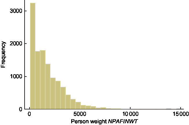
Fig. 1 Histogram of the person (sampling) weight variable NPAFINWT, n 12 153
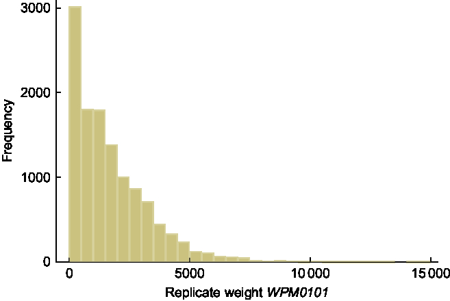
Fig. 2 Histogram of the first replicate weight variable WPM0101, n 12 153
Statistical analysis
Estimating descriptive statistics and their se for a mixture of variable types was conducted. For the purpose of demonstration, the following variables were selected: continuous variables Height (in cm), Weight (in kg) and BMI; categorical variables Overweight or Obese and Current Smoker. Coefficients for a logistic regression model for the binary variable of Overweight or Obese were also estimated. Three methods of statistical analyses were conducted.
(1) Unweighted: without sampling weights or replicate weights.
(2) Weighted: with sampling weights but without accounting for the complex design; equivalent to weighted analysis assuming simple random sampling.
(3) Complex design: with sampling weights and se estimated accounting for the complex design using a jack-knife procedure with the replicate weights.
Method (1) produces biased estimates of the mean (or percentage) and the associated se; Method (2) produces an unbiased estimate of the mean (or percentage) but a biased estimate of the associated se; whereas Method (3) provides unbiased estimates of the mean (or percentage) and the associated se (Reference Heeringa, West and Berglund5,Reference Wolter11) .
For the three continuous variables, Height (in cm), Weight (in kg) and BMI, the estimated mean and se were determined. A binary variable identifying adults (≥18 years) was first created from the continuous age variable (AGEC); then a binary variable identifying overweight or obese adults was created. For the categorical variable for smoking SMOKEQ1, the percentage of current smokers is estimated for the adult population. A logistic regression model for the status of overweight or obese adults is applied using the covariates: Sex, Age (in years), highest year of school completed (SchEd), total minutes undertaken physical activity in the last week (PhysActMin), remoteness of area category (ARIABC) and current smoker (SMOKEQ1). Reference category: for Sex is male; for SchEd is Year 12 or equivalent; for ARIABC is major city; and for Current Smoker is yes. The statistical software package Stata version 15 was used for all analyses, the commands for mean, proportion and logistic were used with the appropriate svy command settings for the three methods given in the appendices. The sixty jack-knife replicate weight variables are defined in Stata with the jkrweight option in the svyset command.
The formulas used for the three methods are shown here for the estimates of the population mean and its variance.
(1) Unweighted: the familiar sample mean of a single variable y, denoted by
 $$\bar y$$
, and its estimated variance assuming a simple random sample without replacement of size n from a target population of size N, and sample variance s
2, are calculated without the sampling weights or the replicate weights. If y
i
is the ith observation (
$i = 1, \ldots ,n$
) from the sample, then the sample mean and estimated variance are given by:$${\bar y} = {1 \over n}\sum\limits_{i = 1}^n {{y_i}} ,$$
and$$v(\bar y) = \left( {1 - {n \over N}} \right){{{s^2}} \over n}$$
and the se is calculated by$${s^2} = {1 \over {n - 1}}\sum\limits_{i = 1}^n {{{\left( {{y_i} - \bar y} \right)}^2}} ,$$
$\sqrt {v(\bar y)} $
.
$$\bar y$$
, and its estimated variance assuming a simple random sample without replacement of size n from a target population of size N, and sample variance s
2, are calculated without the sampling weights or the replicate weights. If y
i
is the ith observation (
$i = 1, \ldots ,n$
) from the sample, then the sample mean and estimated variance are given by:$${\bar y} = {1 \over n}\sum\limits_{i = 1}^n {{y_i}} ,$$
and$$v(\bar y) = \left( {1 - {n \over N}} \right){{{s^2}} \over n}$$
and the se is calculated by$${s^2} = {1 \over {n - 1}}\sum\limits_{i = 1}^n {{{\left( {{y_i} - \bar y} \right)}^2}} ,$$
$\sqrt {v(\bar y)} $
.(2) Weighted: If the sampling weight for an individual in the sample is denoted by w i (
$i = 1, \ldots ,n$
) and the weights are calibrated to sum to the population size N,
$\sum\nolimits_{i = 1}^n {{w_i} = N} ,$
the estimator of the population mean is the mean of the weighted observations; and the variance is the equivalent to weighted analysis assuming simple random sampling, such that:and$$\hat \theta = {{\sum\nolimits_{i = 1}^n {{w_i}{y_i}} } \over {\sum\nolimits_{i = 1}^n {{w_i}} }}$$
$$v\left( {\hat \theta } \right) = \left( {1 - {n \over N}} \right)\left( {{n \over {n - 1}}} \right){1 \over {{N^2}}}\sum\limits_{i = 1}^n {w_i^2{{\left( {{y_i} - \hat \theta } \right)}^2}} .$$
(3) Complex design: the sample weights are used to calculate the weighted mean as given in Method (2) above. The replicate weight variable for each replicate group is used to obtain the R replicate estimates of the mean, resulting in
${\hat \theta _1}, \ldots ,{\hat \theta _R}$
. The variance estimate of
$\hat \theta $
is then given by
${v^ * }\left( {\hat \theta } \right)\hskip-4pt:$
(1)where the jack-knife multiplier, m, is given by$${v^ * }\left( {\hat \theta } \right) = m\sum\limits_{r = 1}^R {{{\left( {{{\hat \theta }_r} - \hat \theta } \right)}^2}} ,$$
$m = {{\left( {R - 1} \right)} \mathord{\left/ {\vphantom {{\left( {R - 1} \right)} R}} \right.} R}.$
For the AHS data, a delete-a-group jack-knife method of replicate weighting is used producing R = 60 replicate weights, so m = 59/60(12).


The jack-knife variance estimator
 ${v^ * }\left( {\hat \theta } \right)$
is centred on the overall estimate obtained using the individual sampling weights for the whole sample (assuming they are provided). An alternative is to use the average of the replicate estimates, which has to be used if the individual weights are not available, allowing centring on the average of the estimates only. Wolter(Reference Wolter11) (p. 170) notes that for linear estimates these alternatives are identical and in general either approach can be used, with
${v^ * }\left( {\hat \theta } \right)$
is centred on the overall estimate obtained using the individual sampling weights for the whole sample (assuming they are provided). An alternative is to use the average of the replicate estimates, which has to be used if the individual weights are not available, allowing centring on the average of the estimates only. Wolter(Reference Wolter11) (p. 170) notes that for linear estimates these alternatives are identical and in general either approach can be used, with
 ${v^ * }\left( {\hat \theta } \right)$
giving larger variance estimates.
${v^ * }\left( {\hat \theta } \right)$
giving larger variance estimates.
For the coefficients in a logistic regression, the variance of the unweighted estimates was estimated using standard methods(Reference Heeringa, West and Berglund5). For weighted analysis, the variance ignoring the sample design was estimated using a linearization approach(Reference Binder18). The jack-knife approach uses
 ${v^ * }\left( {\hat \theta } \right)$
defined in equation (1), where
${v^ * }\left( {\hat \theta } \right)$
defined in equation (1), where
 ${\hat \theta _r}$
is the estimate of the coefficient obtained using the weights for replicate r.
${\hat \theta _r}$
is the estimate of the coefficient obtained using the weights for replicate r.
Estimates for subgroups
Often a researcher is interested in estimating a quantity such as a mean or proportion for a subgroup of the population (sometimes referred to as a domain or a sub-population); for example, the mean BMI by Sex may be of interest. In the present paper, we are focusing on how to carry out such analyses when the replicate weights have been supplied and the jack-knife replication method to variance estimation is to be applied. In this situation the data analyst has two options, both achieving the same results when a jack-knife approach is used:
(a) use a binary variable to identify the subgroup in the full sample; or
(b) use a conditional if statement to restrict the sample to the required subgroup or, equivalently, split the data set.
Valliant et al.(Reference Valliant, Dever and Kreuter1) (p. 421) note that the jack-knife correctly handles subgroup estimation without the need to explicitly give people not in the subgroup a zero response variable; that is, it is not necessary to create a binary variable to identify the subgroup in the full sample. However, as Valliant et al. (p. 410)(Reference Valliant, Dever and Kreuter1) explain, Option (a) may produce different results when a Taylor linearization approach (Approach (A)) is applied (i.e. when accounting for the sample design using the sample design variables). If the subgroup is not fixed by the design of the survey (i.e. not defined by a particular stratum, for example) then the sample size for the subgroup is random and should be incorporated into the variance estimates. In a Taylor linearization approach, this can be achieved by applying Option (a) rather than Option (b). Interested readers are referred to West et al.(Reference West, Berglund and Heeringa19) who explain the conceptual differences between these methods for the Taylor linearization approach.
As the data analyst using the replicate weights may choose between Options (a) and (b), it is recommended that the full data set be used for good practice (Option (a)), rather than restricting the data to the particular cases belonging to the subgroup or splitting the data set (Option (b)). The Stata manual for survey data(7) describes using command options subpop and over when estimating parameters for subgroups of the population rather than restricting the number of cases using conditional if or in qualifiers. The subpop option can be used to break down estimates into two groups using either a binary variable with zero/non-zero values such as 0/1 or using an if qualifier within the subpop command. The over option allows a breakdown by a categorical variable with two or more categories. For demonstration, the subgroup analyses for the mean Height (in cm), Weight (in kg) and BMI by Sex and the proportions of Overweight or Obese and Current Smoker by Sex are conducted using both Options (a) and (b), with Stata code shown in the appendices.
Results
The results for the descriptive statistics for the five chosen variables are listed in Table 2 for all adults and for the subgroups analysis by gender, using both Options (a) and (b) described above. As the same estimated se is produced for complex design estimates using both subgroup options, the results are only reported here once. The unweighted point estimates of the means and percentages (Method (1)) are biased and will therefore differ from the unbiased point estimates produced by the weighted (Method (2)) and complex design (Method (3)) methods. However, the point estimates calculated with Methods (2) and (3) are equal as expected, since they use the same formula incorporating the sampling weights. For Height the biased unweighted mean is lower but for the other variables, it is higher. The estimated se across the three methods are different, with Method (3) producing the only unbiased se. The se for Method (2) are larger than for Method (1), reflecting the higher variability between the observations when weighted. The differences between estimated se for Methods (2) and (3) are interesting as they highlight the change in the estimated se which occurs from properly taking account of the complex sample design used in the survey. For Height, Weight and BMI, se have all decreased, except for Weight for males. However, increases in se are evident for Overweight or Obese (such as 0·74–0·78 for all adults) and for Current Smoker (such as 0·80–0·84 for males) but not for females.
Table 2 Results for estimates of mean Height (in cm), Weight (in kg), BMI, percentage of Overweight or Obese adults (BMI ≥ 25 kg/m2) and percentage of Current Smokers for all adults, males (M) and females (F), and associated se, shown for three methods: (1) unweighted; (2) weighted; and (3) complex design using a jack-knife procedure with the replicate weights

* Different sample sizes reflect the number of responding adults for the variable listed. Total number of adults in the sample is 9435; 4329 are male (M) and 5106 are female (F).
The results for the logistic regression model of whether or not an adult is Overweight or Obese are provided in Table 3. The OR estimate, the estimated se, the t statistic, the related P value and the 95 % CI are reported for each of the three methods. The results for the unweighted analysis, Method (1), provide biased OR estimates and so differ from the unbiased estimates shown for Methods (2) and (3).
Table 3 Results for logistic regression (OR, se, t statistic, related P value and 95 % CI) for all adults (n 7874): whether or not an adult is Overweight or Obese given six explanatory variables is shown for three methods: (1) unweighted; (2) weighted; and (3) complex design using a jack-knife procedure with the replicate weights

Reference category: for Sex is male; for SchEd is Year 12 or equivalent; for ARIABC is major city; for Current Smoker is yes.
The estimated se for the corresponding covariates differ across the three methods as expected. Again, it is clear that for Method (2), the se are all higher than those for Method (1), but these are both biased se. All but one of the estimated se are higher for the complex design results by Method (3) than for the weighted results by Method (2); with the se for Current Smoker being the exception. The most notable difference is for the covariate Current Smoker. For Current Smoker, the unweighted method gives an OR = 1·20 which is statistically significantly higher than 1·0 (assuming a 5 % level) with t = 2·89, P = 0·004 and 95 % CI (1·061, 1·365). However, for the complex design which produces unbiased OR and se estimates, Method (3), the result is not statistically significant with t = 0·71, P = 0·480 and 95 % CI (0·894, 1·267), underlining that invalid inferences can be made if analysis does not take the complex design into account. Also noteworthy are the results for the variable for remoteness of area category (ARIABC). Method (1) reports, for the Other category, se = 0·081, t = 2·03 and P = 0·043, whereas the corresponding results for Method (3) give se = 0·146, t = 2·47 and P = 0·016. The results for Method (2) are similar to those for Method (3), with the unbiased estimated se slightly higher for Method (3).
To summarise the different se between methods for the same covariate, the ratio of the estimated se for Method (2) to the se for Method (1) found a minimum ratio of 1·12 (for Current Smoker – No), a maximum of 1·78 (for ARIABC – Other) and a median of 1·36 across the covariates. The ratio of the estimated se for Method (3) to the se for Method (2) found a minimum of 0·99 (for Current Smoker – No), a maximum of 1·19 (for SchEd – Year 10) and a median of 1·07.
Discussion
When reading the literature on secondary analyses of national health surveys, it can be unclear whether the reported estimates are the weighted estimates and whether the analysis accounted for the complex survey design, for example by using unbiased estimates of se. Bell et al.(Reference Bell, Onwuegbuzie and Ferron4) carried out a review of 1003 published papers reporting empirical research from 1995 to 2010 in three health surveys. They found that ‘60 % of articles reported accounting for design effects and 61 % reported using sample weights’. For an Australian example, Allman-Farinelli et al.(Reference Allman-Farinelli, Chey and Merom20) examined BMI and the prevalence of overweight and obesity by occupation using NHS 2004–2005 data collected by the Australian Bureau of Statistics. The person sampling weights were used in the analysis, but there is no mention of the method used to obtain the reported se that account for the complex sample design and how the restriction to adults aged 20–64 years was handled. The AHS data from 2011 to 2012 were used in a study on cardiovascular health by Peng et al.(Reference Peng, Wang and Dong21). Poisson and logistic regression analyses were conducted on a restricted subgroup of the core sample with analysis applying the biomedical sample weights and jack-knife method for variance estimation as recommended by the Australian Bureau of Statistics(22).
Saylor et al.(Reference Saylor, Friedmann and Lee8) demonstrate the importance of using the sampling weights and accounting for the survey’s complex sample design in any statistical analysis with particular reference to the NHANES 2007–2008. The sample design variables for NHANES, including the stratification and cluster variables, are supplied in the data files in addition to the sampling weight variable. The authors undertake analyses in the SPSS statistical software package, including descriptive statistics, linear and logistic regression, using three methods: unweighted, weighted and complex samples. They illustrate that the mean age obtained from an unweighted analysis is 51·15 (se = 0·348) years whereas a complex samples analysis obtains a mean age of 46·91 (se = 0·595) years; the difference in the mean is due mostly to the higher sampling rate in the ≥60 years age group and the difference in the estimated se is due to the complex sample design. Results are also provided for a mean estimate for diet (in kcal/d) of 2032·15 (se = 19·707) for unweighted analysis compared with 2150·45 (se = 37·109) for a complex samples analysis. They conclude that accurate parameter estimates are produced if using weights without the complex sample design information but that ‘weighting alone leads to inappropriate population estimates of variability’(Reference Saylor, Friedmann and Lee8) (p. 236).
Similarly, Kim et al.(Reference Kim, Park and Kim9) report that only 19·8 % of the 247 research articles using data from the Korean NHANES cited in PubMed from 2007 to 2012 correctly used survey analysis accounting for the design. Using SAS and SUDAAN statistical software packages, these researchers(Reference Kim, Park and Kim9) compare the estimates of levels of lead, cadmium and mercury in the blood and the associated se as well as OR (and 95 % CI) for hypertension and osteoporosis for particular subgroups, using both unweighted and a weighted analysis accounting for the complex design. The results highlight the differences in the parameter estimates if weighting is not applied and the tendency for se to be underestimated and the CI to be invalid.
The weighted simple random sampling se estimator, Method (2), treats the data as a simple random sample of weighted values. This estimator at least partially accounts for the use of weights but does not reflect the effect of stratification and clustering in the sample design or the use of post-stratification in the estimation. Ignoring the effect of stratification may mean that the estimator will tend to overestimate the true se, while ignoring the clustering and post-stratification will tend to underestimate the se. The net effect of these factors will depend on the particular design used, for example how the sampling rate varies between strata, the extent of the clustering in the design and the variable being considered (see Section 2.6.3 in Heeringa et al.(Reference Heeringa, West and Berglund5)). It is possible for the weighted simple random sampling se estimator, Method (2), to be larger or smaller than the se estimates obtained using the replicate weights, Method (3), which properly account for these effects. The clustering in the AHS is not high, with an average of less than 7 dwellings selected per PSU and so we would not expect a large increase in se due to the clustering in the sample, but some increase is evident in the complex variance analysis. If the sample design has a high degree of clustering, the effect on the se may be large(Reference Burden, Probst and Steel23). The sample size is a major determinant of the true se, with further effects due to the weighting and the complex design (see Chapter 1 in Wolter(Reference Wolter11)), which are accounted for in Method (3). Whether the estimated se is smaller or larger in Method (3) than the other methods, this method will provide an unbiased estimate of the se allowing the corresponding CI to be used to make valid inferences.
Conclusion
The present paper discusses the results of three approaches to secondary analysis of complex survey data which have replicate weight variables supplied rather than the sample design variables, such as the variables indicating the strata and cluster to which people belong. These are important considerations for nutrition-related analyses in surveys employing replicate weights.
The first question was: What happens if I don’t use the sampling weights or the design information in my analysis? If the sampling weights are not used in the analysis, biased point estimates (or estimated parameters) are produced, demonstrated by the differences in the estimates produced by the unweighted and weighted methods. In addition, if the complex design is not included, which corresponds to not using the replicate weights, the estimated se will also be biased. The use of these incorrect point estimates and se may result in incorrect inferences and conclusions. For valid inferences, the best estimates are those accounting for both the sampling weights and sample design information.
The second question was: How do I carry out analyses such as estimation of means, proportions and their se; and estimates of coefficients for a logistic regression model? The present paper demonstrates the use of replicate weights for analysing complex survey data using the AHS data which include sixty replicate weight variables. Other researchers of AHS data or other surveys with replicate weights may use this analysis as an example.
The third question was: How do I obtain estimates for subgroups when data is sampled using a complex survey design? Two options are available to the analyst when the replicate weights are supplied; thereby showing that Approach (B) using the replicate weights is robust and simplifies procedures for the analyst. However, for good practice, we suggest that the analyst becomes familiar with Option (a).
The last question was: How do I set up the code to incorporate the replicate weights in Stata? The Stata code provided in Appendices 1 and 2 may be used as an example for researchers performing similar analysis. The analyst is referred to the user’s guide for the particular survey to determine the type of replication method and the number of replicate weights to apply. For further examples, see Chapter 5 in Valliant and Dever(Reference Valliant and Dever3).
Acknowledgements
Acknowledgements: The authors would like to thank the Associate Editor and reviewer for their valuable comments. Financial support: This research received no specific grant from any funding agency in the public, commercial or not-for-profit sectors. Conflict of interest: None of the authors has any conflict of interest to declare. Authorship: C.L.B. and A.A. performed the research and analysis; C.L.B., D.G.S. and M.J.B. wrote the paper. Ethics of human subject participation: Not applicable.
Appendix 1
Stata code: estimates of means and proportions
The code in this appendix relates to the results in Table 2. In the AHS data, some variables have been given missing codes of 98, 99, 997, 998 and 999 which are defined in the microdata CURF data item list supplied with the data. These values were replaced with appropriate codes for missing observations in Stata such as .a, .b and .c. For convenience, the variable for weight (PHDKGWBC) was renamed to Weight_kg. Similarly, the variable for height (PHDCMHBC) was renamed to Height_cm. The code for the data preparation is given below.
A dummy variable to indicate adults was created:

A dummy variable to indicate the BMI category of overweight or obese was also created:
Method (1): Unweighted
Unweighted results are obtained using standard procedures without sampling weights or accounting for design features.
Alternatively, the same results may be obtained by applying the svy commands as provided in the following ‘Method (2): Weighted’ subsection below, but replacing the svyset commands to assume simple random sampling as follows:
Method (2): Weighted
Weighted results include the sampling weights but do not account for the complex sample design. NPAFINWT are the individual sampling weights supplied with the data.

Method (3): Complex design
Results for Method (3) are weighted and account for the complex design using the replicate weights: utilising the sampling weights,NPAFINWT, and the sixty replicate weights, WPM0101–WPM0160, supplied with the data. The results may be obtained by replacing the svyset commands in the above ‘Method (2): Weighted’ subsection with the following three lines. All other svy code remains the same as above:
Appendix 2
Stata code: logistic regression
The code in this appendix relates to the results in Table 3.
For convenience, the following variables were renamed: LVHNSQBC was renamed to NonSchEd; HYSCHCBC was renamed to SchEd; and EXLEVELN was renamed to PhysActMin.
Method (1): Unweighted
Method (2): Weighted
Method (3): Complex design


