


1 INTRODUCTION
Systematic studies of star clusters help us to understand the Galactic structure and star formation processes as well as stellar evolution. By utilising colour–magnitude diagrams of the stars observed in the optical/near-infrared (NIR) bands, it is possible to determine the underlying properties of the clusters such as age, metallicity and distance. Colour–magnitude diagrams of star clusters can be used as a good distance indicator. The distance to a star can be evaluated by trigonometric or photometric parallaxes. Trigonometric parallaxes are only available for nearby stars where Hipparcos (ESA 1997) is the main supplier for the data. For stars at large distances, the use of photometric parallaxes is unavoidable. In other words, the study of the Galactic structure is strictly tied to the precise determination of absolute magnitudes.
Different methods can be used for absolute magnitude determination, where most of them are devoted to dwarfs. The method used in the Strömgren’s uvby–β (Nissen & Schuster Reference Nissen and Schuster1991) and in the UBV (Laird, Carney, & Latham Reference Laird, Carney and Latham1988) photometry depends on the absolute magnitude offset from a standard main sequence. In recent years, the derivation of absolute magnitudes has been carried out by means of colour–absolute magnitude diagrams of some specific clusters whose metal abundances are generally adopted as the mean metal abundance of a Galactic population, such as thin, thick discs and halo. The studies of Phleps et al. (Reference Phleps, Meisenheimer, Fuchs and Wolf2000) and Chen et al. (Reference Chen2001) can be given as examples. A slightly different approach is that of Siegel et al. (Reference Siegel, Majewski, Reid and Thompson2002), where two relations, one for stars with solar-like abundances and another for metal-poor stars, were derived between MR and the colour index R−I, where MR is the absolute magnitude in the R filter of the Johnson system. For a star of given metallicity and colour, absolute magnitude can be estimated by linear interpolation of two ridgelines and by means of linear extrapolation beyond the metal-poor ridgeline.
The most recent procedure used for absolute magnitude determination consists of finding the most likely values of the stellar parameters, given the measured atmospheric ones, and the time spent by a star in each region of the H–R diagram. In practice, researchers select the subset of isochrones with [M/H]±Δ[M/H], where Δ[M/H] is the estimated error on the metallicity, for each set of derived T eff, log g and [M/H]. Then, a Gaussian weight is associated with each point of the selected isochrones, which depends on the measured atmospheric parameters and the errors considered. This criterion allows the algorithm to select only the points whose values are closed by the pipeline. For details of this procedure, we cite the works of Breddels et al. (Reference Breddels2010) and Zwitter et al. (Reference Zwitter2010). This procedure is based on many parameters. Hence, it provides absolute magnitudes with high accuracy. Also, it can be applied to both dwarf and giant stars simultaneously.
In Karaali et al. (Reference Karaali, Karataş, Bilir, Ak and Hamzaoğlu2003), we presented a procedure for the photometric parallax estimation of dwarf stars which depends on the absolute magnitude offset from the main sequence of the Hyades cluster. Bilir et al. (Reference Bilir, Karaali, Ak, Yaz, Cabrera-Lavers and Coşkunoğlu2008) obtained the absolute magnitude calibrations of the thin disc main-sequence stars in the optical MV and in the NIR MJ bands using the recent reduced Hipparcos astrometric data (van Leeuwen Reference van Leeuwen2007). Bilir et al. (Reference Bilir, Karaali, Ak, Coşkunoğlu, Yaz and Cabrera-Lavers2009) derived a new luminosity colour relation based on trigonometric parallaxes for the thin disc main-sequence stars with Sloan Digital Sky Survey (SDSS) photometry. Yaz et al. (Reference Yaz, Bilir, Karaali, Ak, Coşkunoğlu and Cabrera-Lavers2010) obtained transformation between optical and NIR bands for red giants. Bilir et al. (Reference Bilir, Karaali, Daǧtekin, Önal, Ak, Ak and Cabrera-Lavers2012) extended this study to mid-infrared bands by using Radial Velocity Experiment (RAVE) Third Data Release (DR3) data (Siebert et al. Reference Siebert2011). Both works provide absolute magnitudes for a given photometry from another one.
In Karaali, Bilir, & Yaz Gökçe (Reference Karaali, Bilir and Yaz Gökçe2012a, Reference Karaali, Bilir and Yaz Gökçe2012b; hereafter Paper I and Paper II, respectively), we used a procedure for the absolute magnitude estimation of red giants by using the V 0×(B−V)0 and g 0×(g−r)0 apparent magnitude–colour diagrams of Galactic clusters with different metallicities. Here, we extend our procedure to Two Micron All Sky Survey (2MASS; Skrutskie et al. Reference Skrutskie2006) photometry. We aim to estimate MJ and MK s absolute magnitudes for red giants with J 0×(V−J)0 and K s 0 × (V−K s 0 colour–magnitude diagrams. The outline of the paper is as follows. We present the data in Section 2. The procedure used for calibration is given in Section 3, and Section 4 is devoted to summary and discussion.
2 DATA
We calibrated two different absolute magnitudes, MJ and MK s, in terms of metallicity. Hence, we used two different sets of data. The calibration of MJ with J 0 and (V−J)0 is given in Section 2.1, whereas that for MK s with K s 0 and (V−K s)0 is presented in Section 2.2.
2.1 Data for Calibration with J 0 and (V−J)0
Five clusters with different metallicities, i.e. M92, M13, M71, M67, and NGC 6791, were selected for our program (Table 1). The V magnitudes and V−J colours for the clusters M92, M13, and M71 were taken from the tables in Brasseur et al. (Reference Brasseur, Stetson, VandenBerg, Casagrande, Bono and Dall’Ora2010), whereas the data for the clusters NGC 6791 and M67 could be provided by different procedures as explained in the following. We used Figure 1 of Brasseur et al. (Reference Brasseur, Stetson, VandenBerg, Casagrande, Bono and Dall’Ora2010) and obtained a set of 30 [MV , (V−J)0] couples for the red giant branch (RGB) of the cluster NGC 6791. Then, we transformed the MV absolute magnitudes to V apparent magnitudes by means of the apparent distance modulus of the cluster, i.e. μ=13.25 mag. Finally, we de-reddened the V magnitudes and combined them with the true colour indices (V−J)0 and obtained J 0 magnitudes. The J 0 magnitudes and (V−J)0 colours are not available for the cluster M67 in the literature. Hence, we transformed the V, B−V and V−I data in Montgomery, Marschall, & Janes (Reference Montgomery, Marschall and Janes1993) to obtain a set of (J 0, (V−J)0) data for the RGB of M67. It turned out that 21 of the stars in the bright stars catalogue in Montgomery et al. (Reference Montgomery, Marschall and Janes1993) were red giants. We de-reddened the V, B−V, and V−I data of these stars and transformed them to (V−J)0 colours by using the following equation of Yaz et al. (Reference Yaz, Bilir, Karaali, Ak, Coşkunoğlu and Cabrera-Lavers2010):
 \begin{eqnarray}
(V-J)_{0} & = & 1.080(B-V)_{0}+0.379(V-I)_{0}\nonumber \\
&&- \, 0.082[{\rm Fe/H}]+0.279.
\end{eqnarray}
\begin{eqnarray}
(V-J)_{0} & = & 1.080(B-V)_{0}+0.379(V-I)_{0}\nonumber \\
&&- \, 0.082[{\rm Fe/H}]+0.279.
\end{eqnarray}
Then, we combined them with the V 0 magnitudes and obtained the J 0 ones.
Table 1. Data for Five Clusters

Notes. We used the data in the first line for each cluster for absolute magnitude calibration, whereas those in the second and third lines are for comparison purposes. l and b are the Galactic longitude and latitude of the clusters; the symbol μ0 indicates the true distance modulus of the cluster. References: (1) Gratton et al. (Reference Gratton, Pecci, Carretta, Clementini, Corsi and Lattanzi1997); (2) Harris (Reference Harris2010); (3) Brasseur et al. (Reference Brasseur, Stetson, VandenBerg, Casagrande, Bono and Dall’Ora2010); (4) Hodder et al. (Reference Hodder, Nemec, Richer and Fahlman1992); (5) Sarajedini, Dotter, & Kirkpatrick (Reference Sarajedini, Dotter and Kirkpatrick2009); (6) Hog & Flynn (Reference Hog and Flynn1998); (7) Anthony-Twarog, Twarog, & Mayer (Reference Anthony-Twarog, Twarog and Mayer2007); (8) Sandage, Lubin, & VandenBerg (Reference Sandage, Lubin and VandenBerg2003).
We adopted R=AV /E(B−V)=3.1 to convert the colour excess to the extinction. Although different numerical values appeared in the literature for specific regions of our Galaxy, a single value is applicable everywhere. Then, we used the equations E(V−I)/E(B−V)=1.25 and E(V−J)/E(B−V)=2.25 of Fiorucci & Munari (Reference Fiorucci and Munari2003) and McCall (Reference McCall2004), respectively, to evaluate the colour excesses in V−I and V−J colours. The intrinsic colours were evaluated by the equations (V−I)0=(V−I)−E(V−I) and (B−V)0=(B−V)−E(B−V).

Figure 1. J 0×(V−J)0 colour–apparent magnitude diagrams for five Galactic clusters used for the absolute magnitude calibration.
We adopted different equations, i.e. R=AV /E(B−V)=4.0 (Turner Reference Turner2012) and E(V−J)/E(B−V)=2.30 (Smith Reference Smith1987), and evaluated the corresponding E(V−J) selective and AJ =1.70E(B−V) total absorptions for the clusters [we do not give the calculations here, only we remind to the reader that E(V−J) is equivalent to AV −AJ ]. The results are given in Table 2. The differences between the E(V−J) colour excesses estimated in our study and the ones in this paragraph are rather small. The same case holds for the AJ total absorptions except those for M71 and NGC 6791, i.e. ΔAJ ~0.2 and 0.1, respectively, whose E(B−V) colour excesses are slightly larger. We should add that the extinction equation of Turner (Reference Turner2012) was derived for low Galactic latitudes, i.e. the Carina region (b~0°). Whereas the Galactic latitudes of the clusters used in our study are (absolutely) greater than b=4°.5 (see Table 1). Hence, the extinction ratio and the colour excess ratios used in our study are preferable.
Table 2. Comparison of the Selective and Total Absorptions Evaluated by Using Different Extinction and Colour Excess Ratios

Notes. Description of columns: (1) the cluster; (2) adopted E(B−V) colour excess; (3) E(V−J) p , the colour excess evaluated by the equation E(V−J)/E(B−V)=2.25 and used in the paper; (4) E(V−J) c , the colour excess evaluated by the equation E(V−J)/E(B−V)=2.30 for comparison purposes; (5) ΔE(V−J), the difference between the colour excesses in columns (3) and (4); (6) (AJ ) p , the total absorption evaluated by the equation AJ /E(B−V)=0.87 and used in the paper; (7) (AJ ) c , the total absorption evaluated by the equation AJ /E(B−V)=1.70; and (8) ΔAJ , the difference between the total absorptions in columns (6) and (7).
The range of the metallicity of the clusters in iron abundance is −2.15≤[Fe/H]≤+0.37 dex. The μ0 true distance modulus, E(B−V) colour excess, and [Fe/H] iron abundance for M92, M13, M71, and M67 were taken from Paper I, whereas those for the cluster NGC 6791 are taken from Brasseur et al. (Reference Brasseur, Stetson, VandenBerg, Casagrande, Bono and Dall’Ora2010), except the metallicity which is adopted from Paper I. These data are given in Table 1, whereas the J 0 magnitudes and (V−J)0 colours are presented in Table 3. We then fitted the fiducial sequence of the red giants to a fourth-degree polynomial for all clusters. The calibration of J 0 is as follows:
 \begin{eqnarray}
J_{0}= \sum _{i=0}^{4}a_{i}(V-J)^{i}_0.
\end{eqnarray}
\begin{eqnarray}
J_{0}= \sum _{i=0}^{4}a_{i}(V-J)^{i}_0.
\end{eqnarray}
The numerical values of the coefficients ai (i=1, 2, 3, 4) are given in Table 4 and the corresponding diagrams are presented in Figure 1. The (V−J)0 interval in the second line of the table denotes the range of (V−J)0 available for each cluster.
Table 3. J 0 Magnitudes and (V−J)0 Colours for Five Clusters Used for the Absolute Magnitude Calibration

Note. The last two columns for the cluster M67 indicate the (V−I)0 colours and J 0 magnitudes of the bins used to draw the diagram of M67 in Figure 1.
Table 4. Numerical Values of the Coefficients ai (i=1, 2, 3, 4) in Equation (2)

2.2 Data for Calibration with K s 0 and (V−K s)0
We used the data of the same clusters as mentioned in Section 2.1, i.e. M92, M13, M71, M67, and NGC 6791, for calibration of the MK s absolute magnitudes. We adopted the same colour excesses, distance moduli, and metallicities as in Table 1. The K s 0 magnitudes and (V−K s)0 colours for the clusters M92, M13, and M71 were taken from the tables of Brasseur et al. (Reference Brasseur, Stetson, VandenBerg, Casagrande, Bono and Dall’Ora2010). However, we used two different procedures for evaluation of the K s and V−K s data for the clusters M67 and NGC 6791, as explained in the following. For the cluster M67, we transformed the V, B−V, and V−I data of Montgomery et al. (Reference Montgomery, Marschall and Janes1993) to (V−K s)0 by the following equation of Yaz et al. (Reference Yaz, Bilir, Karaali, Ak, Coşkunoğlu and Cabrera-Lavers2010), and then we evaluated the K s 0 magnitudes by the combination of V 0 magnitudes and (V−K s)0 colours:
 \begin{eqnarray}
(V-K_{\rm s})_{0} & = & 1.791(B-V)_{0}+0.294(V-I)_{0}\nonumber \\
&& -\, 0.129[{\rm Fe/H}]+0.279.
\end{eqnarray}
\begin{eqnarray}
(V-K_{\rm s})_{0} & = & 1.791(B-V)_{0}+0.294(V-I)_{0}\nonumber \\
&& -\, 0.129[{\rm Fe/H}]+0.279.
\end{eqnarray}
The available 2MASS photometric data in Brasseur et al. (Reference Brasseur, Stetson, VandenBerg, Casagrande, Bono and Dall’Ora2010) for the cluster NGC 6791 are the J−K s colours and K s magnitudes, but not the V−K s ones. Hence, we evaluated them by means of the V 0 and J 0 magnitudes for this cluster given in Table 3 in three steps. First, we plotted V 0 magnitudes versus J 0 magnitudes in a diagram (not given here) and obtained the following quadratic equation with a high correlation coefficient, R 2=0.9997:
 \begin{eqnarray}
V_{0}=0.0457J^{2}_{0}-0.3744J_{0}+12.9000.
\end{eqnarray}
\begin{eqnarray}
V_{0}=0.0457J^{2}_{0}-0.3744J_{0}+12.9000.
\end{eqnarray}
In the second step, we evaluated the J magnitudes by combining J−K s and K s, and finally we de-reddened the J magnitudes and transformed them to V 0 magnitudes by Equation (4). We used the equations AJ /E(B−V)=0.87 and AK s/E(B−V) = 0.38 of Savage & Mathis (Reference Savage and Mathis1979) for de-reddening of the magnitudes J and K s, respectively. As Equation (4) is defined for 9.94≤J 0≤15.06, we could not consider five bright J 0 magnitudes in Table 3. The (V−K s)0 and K s 0 data for the clusters are given in Table 5.
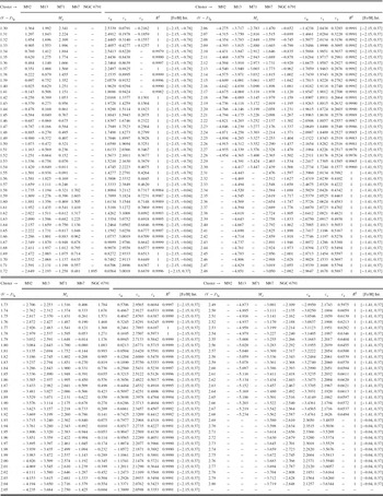
Table 5. K s 0 Magnitudes and (V−K s)0 Colours for Five Clusters Used for the Absolute Magnitude Calibration

Note. The last two columns for the cluster M67 indicate the (V−K s)0 colours and K s 0 magnitudes of the bins used to draw the diagram of M67 in Figure 2.
As in Section 2.1, we adopted different equations, i.e. R=AV /E(B−V)=4.0 (Turner Reference Turner2012), E(J−H)/E(B−V)=0.295, E(H−K s)/E(J−H)=0.49 (Turner Reference Turner2011), and evaluated the corresponding E(V−K s)=2.74E(B−V) selective and AK s=1.26E(B−V) total absorptions for the clusters. The results are given in Table 6. The differences in E(V−K s) and ΔAK s are almost the same as in Table 2. We prefer the extinction ratio and the colour excess ratios used in our study due to the reason explained in Section 2.1.
Table 6. Comparison of the Selective and Total Absorptions Evaluated by Using Different Extinction and Colour Excess Ratios

Notes. Description of columns: (1) the cluster; (2) adopted E(B−V) colour excess; (3) E(V−K s) p , the colour excess evaluated by the equation E(V−K s)/E(B−V)=2.72 used in the paper; (4) E(V−K s) c , the colour excess evaluated by the equation E(V−K s)/E(B−V)=2.74 for comparison purposes; (5) ΔE(V−K s), the difference between the colour excesses in columns (3) and (4); (6) (AK s) p , the total absorption evaluated by the equation AK s/E(B−V) = 0.38 used in the paper; (7) (AK s)c, the total absorption evaluated by the equation AK s/E(B−V)=1.26; and (8) ΔAK s, the difference between the total absorptions in columns (6) and (7).
We fitted the (V−K s)0 colours and K s 0 magnitudes to a fourth-degree polynomial for all clusters, except M67 for which a fifth-degree polynomial provided a higher correlation coefficient. The calibration of K s 0 is as follows:
 \begin{eqnarray}
K_{{{\rm s}}_0}=\sum _{i=0}^{5}b_{i}(V-K_{\rm s})^{i}_0.
\end{eqnarray}
\begin{eqnarray}
K_{{{\rm s}}_0}=\sum _{i=0}^{5}b_{i}(V-K_{\rm s})^{i}_0.
\end{eqnarray}
The numerical values of the coefficients bi (i=1, 2, 3, 4, 5) are given in Table 7 and the corresponding diagrams are presented in Figure 2. The (V−K s)0 interval in the second line of the table indicates the range of (V−K s)0 available for each cluster.
Table 7. Numerical Values of the Coefficients bi (i=1, 2, 3, 4, 5) in Equation (5)

*The (V−K s)0 domain of the cluster M71 is in fact [1.79, 4.63]. However, we restricted it with an upper limit of 3.10 mag due to some uncertainties claimed by the authors.
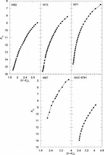
Figure 2. K s 0 × (V−K s)0 colour–apparent magnitude diagrams for five Galactic clusters used for the absolute magnitude calibration.
3 THE PROCEDURE
3.1 Absolute Magnitude as a Function of Metallicity
We adopted the procedure in Paper II, which consists of calibration of an absolute magnitude as a function of metallicity. We calibrated the MJ and MK s, absolute magnitudes in terms of metallicity for a given (V−J)0 and (V−K s)0 colour, respectively.
3.1.1 Calibration of MJ in Terms of Metallicity
We estimated the MJ absolute magnitudes for the (V−J)0 colours given in Table 8 for the clusters M92, M13, M71, M67, and NGC 6791 by combining the J 0 apparent magnitudes evaluated by using Equation (2) and the true distance modulus (μ0) of the cluster in question, i.e.
 \begin{eqnarray}
M_{J}=J_{0}-\mu _{0}.
\end{eqnarray}
\begin{eqnarray}
M_{J}=J_{0}-\mu _{0}.
\end{eqnarray}
Then, we plotted the absolute magnitudes versus (V−J)0 colours. Figure 3 shows that the absolute magnitude is metallicity dependent. It increases (algebraically) with increasing metallicity and decreasing colour.
Table 8. MJ Absolute Magnitudes Estimated for a Set of (V−J)0 Colours for Five Clusters Used in the Calibration


Figure 3. MJ ×(V−J)0 colour–absolute magnitude diagrams for five clusters used for the absolute magnitude calibration.
Now, we can fit the MJ absolute magnitudes to the corresponding [Fe/H] metallicity for a given (V−J)0 colour index and obtain the required calibration. This is carried out for the colour indices (V−J)0= 1.30, 1.60, 1.90, 2.10, 2.25, 2.50, and 2.65 mag just for exhibition of the procedure. The results are given in Table 9 and Figure 4. The absolute magnitudes in all colour indices could be fitted to quadratic polynomials with high (squared) correlation coefficients, i.e. R 2 ≥ 0.9982, including (V−J)0=1.90, 2.10, and 2.25 mag, which cover the largest metallicity range, −2.15≤[Fe/H]≤+0.37 dex. A high correlation coefficient plus (relatively) polynomial with small degree is a strong clue for accurate absolute magnitude estimation.
Table 9. MJ Absolute Magnitudes and [Fe/H] Metallicities for Seven (V−J)0 Intervals
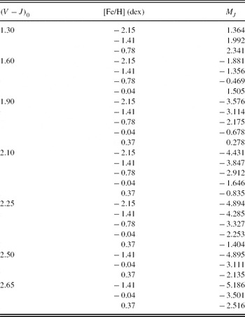
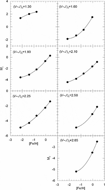
Figure 4. Calibration of the absolute magnitude MJ as a function of metallicity [Fe/H] for seven colour indices.
This procedure can be applied to any (V−J)0 colour interval for which the sample clusters are defined. The (V−J)0 domain of the clusters is different. Hence, we adopted this interval as 1.3≤(V−J)0≤2.8 mag, where at least two clusters are defined, and we evaluated MJ absolute magnitude for each colour. Here, 1.72≤(V−J)0≤2.28 mag is the interval where all the clusters are defined, whereas the range of the interval where only two clusters (M67 and NGC 6791) are defined is rather small, i.e. 2.69≤(V−J)0≤2.80 mag. However, this small interval can be used for estimation of the absolute magnitudes for red giants with metallicities −0.04≤[Fe/H]≤+0.37 dex. The general form of the equation for the calibration is as follows:
 \begin{eqnarray}
M_J=c_{0} + c_{1}X + c_{2}X^{2},
\end{eqnarray}
\begin{eqnarray}
M_J=c_{0} + c_{1}X + c_{2}X^{2},
\end{eqnarray}
where X=[Fe/H]. MJ could be fitted in terms of metallicity by a quadratic polynomial for all (V−J)0 colour intervals with a high correlation coefficient, R 2 ≥ 0.996, except two intervals with small ranges, i.e. a linear fitting was sufficient for the colour intervals 1.34≤(V−J)0≤1.41 and 2.69≤(V−J)0≤2.80 mag where only two clusters are defined. The absolute magnitudes estimated via Equation (7) for 151 (V−J)0 colour indices and the corresponding ci (i=0, 1, 2) coefficients are given in Table 10. However, the diagrams for the calibrations are not given in the paper because of space constraints.
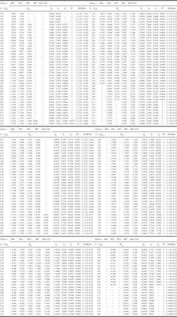
Table 10. MJ Absolute Magnitudes Estimated for Five Galactic Clusters and the Numerical Values of ci (i= 0, 1, 2) Coefficients in Equation (7)
Note. The 11th and 22nd columns give the range of the metallicity [Fe/H] (dex) for the star whose absolute magnitude would be estimated. R 2 is the square of the correlation coefficient.
3.1.2 Calibration of MK s in Terms of Metallicity
We estimated the MK s absolute magnitudes for the (V−K s)0 colours given in Table 11 for the clusters M92, M13, M71, M67, and NGC 6791 by combining the K s 0 apparent magnitudes evaluated by Equation (5) and the true distance modulus (μ0) of the cluster in question, i.e.
 \begin{eqnarray}
M_{{K}_{\rm s}}=K_{{{\rm s}}_0}-\mu _{0}.
\end{eqnarray}
\begin{eqnarray}
M_{{K}_{\rm s}}=K_{{{\rm s}}_0}-\mu _{0}.
\end{eqnarray}
Then, we plotted the absolute magnitudes versus (V−K s)0 colours. Figure 5 shows a similar trend of Figure 3, i.e. the absolute magnitude increases (algebraically) with increasing metallicity and decreasing colour.
Table 11. MK s Absolute Magnitudes Estimated for a Set of (V−K s)0 Colours for Five Clusters used in the Calibration
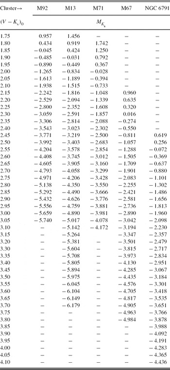
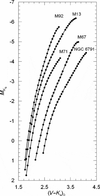
Figure 5. MK s × (V−K s)0 colour–absolute magnitude diagrams for five clusters used for the absolute magnitude calibration.
We fitted the MK s absolute magnitudes to the corresponding [Fe/H] metallicity for the colour indices (V−K s)0= 1.80, 2.00, 2.20, 2.40, 2.60, 3.00, and 3.30 mag just for the exhibition of the procedure. The results are given in Table 12 and Figure 6. We can extend this fitting to a larger (V−K s)0 interval for which the sample clusters are defined. The (V−K s)0 domains of the clusters are different. Hence, we adopted this interval as 1.75 ≤(V−K s)0≤ 3.80 mag where at least two clusters are defined. However, the range of the interval where only two clusters are defined is rather limited, i.e. 1.75≤(V−K s)0≤1.78 and 3.70≤(V−K s)0≤3.80 mag. The common domain of all the clusters is 2.45≤(V−K s)0≤3.04 mag. The general form of the equation for the calibration is as follows:
 \begin{eqnarray}
M_{K_{\rm s}}=d_{0} + d_{1}X + d_{2}X^{2} ,
\end{eqnarray}
\begin{eqnarray}
M_{K_{\rm s}}=d_{0} + d_{1}X + d_{2}X^{2} ,
\end{eqnarray}
where X=[Fe/H]. Note that MK s could be fitted in terms of metallicity by a quadratic polynomial for all (V−K s)0 colour intervals with a high correlation coefficient, R 2 ≥ 0.9972, except two intervals with small ranges, i.e. a linear fitting was sufficient for the colour intervals 1.75≤(V−K s)0≤1.78 and 3.70≤(V−K s)0≤3.80 mag where only two clusters are defined. The absolute magnitudes estimated via Equation (9) for 206 (V−K s)0 colour indices and the corresponding di (i=0, 1, 2) coefficients are given in Table 13. However, the diagrams for the calibrations are not given here because of space constraints.
Table 12. MK s Absolute Magnitudes and [Fe/H] Metallicities for Seven (V−K s)0 Intervals

Table 13. MK s Absolute Magnitudes Estimated for Five Galactic Clusters and the Numerical Values of di (i= 0, 1, 2) Coefficients in Equation (9)
Note. The 11th and 22nd columns give the range of the metallicity [Fe/H] (dex) for the star whose absolute magnitude would be estimated. R 2 is the square of the correlation coefficient.

Figure 6. Calibration of the absolute magnitude MK s as a function of metallicity [Fe/H] for seven colour indices.
The calibration of the absolute magnitude MK s (and MJ ) in terms of [Fe/H] is carried out in steps of 0.01 mag. A small step is necessary to isolate an observational error on the colour V−K s (and V−J) plus an error due to reddening. The origin of the errors mentioned is the trend of the RGB. Although they are not as steep as in BV and gr photometry, a small error in V−K s (and V−J) implies a large change in the absolute magnitude.
Iron abundance, [Fe/H], is not the only parameter that determines the chemistry of the star, but α enhancement, [α/Fe], is also equally important. However, as stated in Paper I, there is a correlation between the two sets of abundances. Hence, we do not expect any considerable change in the numerical values of the estimated absolute magnitudes in the case of addition of the α-enhancement term in Equations (7) and (9).
3.2 Application of the Method
3.2.1 Application of the MJ ×[Fe/H] Calibration
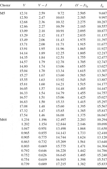
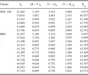
We applied the MJ ×[Fe/H] calibration to the clusters M5 and M68. The reason for choosing clusters instead of field giants is that clusters provide absolute magnitudes for comparison with the ones estimated by means of our method. The J magnitudes and V−J colours for the cluster M5 are taken from Brasseur et al. (Reference Brasseur, Stetson, VandenBerg, Casagrande, Bono and Dall’Ora2010). 2MASS photometric data are not available for the cluster M68. Hence, the J 0 magnitudes and (V−J)0 colours are provided by transformation of the V, B−V, and V−I data of Walker (Reference Walker1994) to J 0 magnitudes and (V−J)0 colours by Equation (1) and the procedure explained in Section 2.1. The data for the clusters are given in Table 14. Two references are given for the cluster M5. The colour excess E(B−V) and the true distance modulus μ0 refer to the first author, whereas the metallicity which was tested in Paper I is taken from the second author. The J 0 magnitudes and (V−J)0 colours as well as the original V, B−V, and V−I data are given in Table 15.
Table 14. Data for the Clusters Used for the Application of the Procedure
References: (1) Brasseur et al. (Reference Brasseur, Stetson, VandenBerg, Casagrande, Bono and Dall’Ora2010); (2) Sandquist et al. (Reference Sandquist, Bolte, Stetson and Hesser1996); (3) VandenBerg & Clem (Reference VandenBerg and Clem2003); (4) Stetson, McClure, & VandenBerg (Reference Stetson, McClure and VandenBerg2004); (5) Meibom et al. (Reference Meibom2009).
Table 15. J 0×(V−J)0 Fiducial Giant Sequences for the Clusters M5 and M68 Used in the Application of the Procedure
We evaluated the MJ absolute magnitude by Equation (7) for a set of (V−J)0 colour indices where the clusters are defined. The results are given in Table 16. The columns refer to (1) (V−J)0 colour index; (2) (MJ )cl, the absolute magnitude for a cluster estimated by its colour–magnitude diagram; (3) (MJ )ev, the absolute magnitude estimated by the procedure; (4) ΔMJ , absolute magnitude residuals. Also, the metallicity for each cluster is indicated near the name of the cluster. The differences between the absolute magnitudes estimated by the procedure presented in this study and those evaluated via colour–magnitude diagrams of the clusters (the residuals) lie in a (relatively) short interval, i.e. −0.08 and +0.34 mag, and the range of 94% of the absolute magnitude residuals is only 0<MJ ≤0.3 mag. The mean and the standard deviation of (all) residuals are 〈ΔMJ 〉=0.137 and σ M J =0.080 mag, respectively. The distribution of the residuals are given in Table 17 and Figure 7.
Table 16. (MJ )ev Absolute Magnitudes and ΔMJ Residuals Estimated by the Procedure Explained in Our Work. (MJ )cl Denotes the Absolute Magnitude Evaluated by Means of the Colour–Magnitude Diagram of the Cluster

Table 17. Distribution of the Residuals. N Denotes the Number of Stars
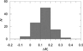
Figure 7. Histogram of the residuals for ΔMJ .
3.2.2 Application of the MK s × [Fe/H] Calibration
NGC 1851 is the last cluster in Brasseur et al. (Reference Brasseur, Stetson, VandenBerg, Casagrande, Bono and Dall’Ora2010) for which K s magnitudes and V−K s colours are available. However, the MK s × (V−K s)0 colour–magnitude diagram of this cluster shows that the uncertainties in the data of this cluster are (relatively) large. Actually, the absolute magnitudes are fainter than the corresponding ones of the cluster M71 for the colour interval (V−K s)0<2.5 mag but brighter for (V−K s)0>2.5 mag. This trend holds for distance modulus and colour excess in Brasseur et al. (Reference Brasseur, Stetson, VandenBerg, Casagrande, Bono and Dall’Ora2010), i.e. μ= 15.50 and E(B−V)=0.034 mag, as well as for alternative data such as E(B−V)=0.02 and μ0=15.50±0.20 mag of Saviane et al. (Reference Saviane, Piotto, Fagotto, Zaggia, Capaccioli and Aparicio1998). If we regard the metallicity claimed by Brasseur et al. (Reference Brasseur, Stetson, VandenBerg, Casagrande, Bono and Dall’Ora2010), [Fe/H]=−1.40 dex, the absolute magnitude colour diagram of the cluster NGC 1851 should coincide with that of M13 ([Fe/H]=−1.41 dex). The alternative metallicity of Rosenberg et al. (Reference Rosenberg, Saviane, Piotto and Aparicio1999), [Fe/H]=−1.03±0.06 dex, should replace the absolute magnitude colour diagram of NGC 1851 between the diagrams of M13 and M71, which is not the case. MK s × (V−K s)0 diagrams for three clusters mentioned in this paragraph are not plotted because of space constraints.
Then, we transformed the V, B−V, and V−I data of NGC 188 (Stetson et al. Reference Stetson, McClure and VandenBerg2004) and M68 (Walker Reference Walker1994) to the K s 0 magnitudes and (V−K s)0 colours by Equation (3) and the procedure explained in Section 2.2. Colour excess E(B−V), distance modulus μ0, and metallicity for the clusters are given in Table 14. The second reference for the cluster NGC 188 is given for the metallicity only, whereas the first reference refers to the colour excess and the distance modulus. The K s 0 magnitudes and (V−K s)0 colours as well as the original V, B−V, and V−I data are given in Table 18.
Table 18. K s×(V−K s)0 Fiducial Giant Sequences for the Clusters NGC 188 and M68 Used in the Application of the Procedure
We evaluated the MK s absolute magnitude by Equation (9) for a set of (V−K s)0 colour indices where the clusters are defined. The results are given in Table 19. The columns refer to (1) (V−K s)0 colour index; (2) (MK s)cl, the absolute magnitude for a cluster estimated by its colour–magnitude diagram; (3) (MK s)ev, the absolute magnitude estimated by the procedure; (4) ΔMK s, absolute magnitude residuals. Also, the metallicity for each cluster is indicated near the name of the cluster. The differences between the absolute magnitudes estimated by the procedure presented in this study and those evaluated via the colour–magnitude diagrams of the clusters (the residuals) lie in a short interval, i.e. −0.10 and +0.27 mag. The mean and the standard deviation of the residuals are 〈 Δ MK s〉 =0.109 and σ M K s=0.123 mag, respectively. The distribution of the residuals is given in Table 20 and Figure 8. The residuals for the cluster NGC 188 for the colour interval 2.15≤(V−K s)0≤2.44, where the metallicity of NGC 188 ([Fe/H]=−0.01 dex) fall off the metallicity interval corresponding to the cited colour interval, −2.15≤[Fe/H]≤−0.04 dex, are slightly larger than those for 2.45≤(V−K s)0≤2.60 where the metallicity interval, −2.15≤[Fe/H]≤+0.37 dex, covers the metallicity of NGC 188. Although the larger residuals are given in Table 19, they are not considered in the statistics.
Table 19. (MK s)ev Absolute Magnitudes and ΔMK s Residuals Estimated by the Procedure Explained in Our Work. (MK s)cl Denotes the Absolute Magnitude Evaluated by Means of the Colour–Magnitude Diagram of the Cluster
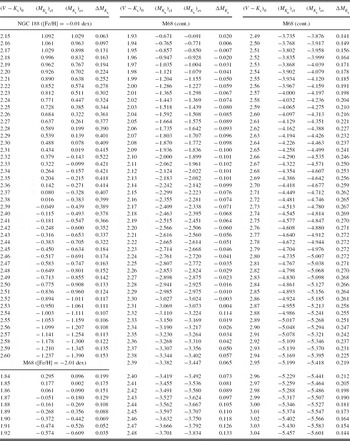
Table 20. Distribution of the Residuals. N Denotes the Number of Stars
Figure 8. Histogram of the residuals for ΔMK s.
4 SUMMARY AND DISCUSSION
We calibrated the absolute magnitudes MJ and MK s for red giants in terms of metallicity by means of the colour–magnitude diagrams of the clusters M92, M13, M71, M67, and NGC 6791 with different metallicities. The J×(V−J) and K s×(V−K s) sequences used for the calibration of MJ and MK s are provided from different sources and by different procedures, as explained in the following. The main source is the paper of Brasseur et al. (Reference Brasseur, Stetson, VandenBerg, Casagrande, Bono and Dall’Ora2010). The J×(V−J) and K s×(V−K s) sequences for the clusters M92, M13, and M71 are taken from the tables of Brasseur et al. (Reference Brasseur, Stetson, VandenBerg, Casagrande, Bono and Dall’Ora2010), whereas the J 0×(V−J)0 sequence for M67 and NGC 6791 is obtained by transformation of V, B−V, and V−I data from Montgomery et al. (Reference Montgomery, Marschall and Janes1993) and by means of the MV ×(V−J)0 diagram from Brasseur et al. (Reference Brasseur, Stetson, VandenBerg, Casagrande, Bono and Dall’Ora2010), respectively. Also, the K s×(V−K s) sequence for M67 is transformed from V, B−V, and V−I data in Montgomery et al. (Reference Montgomery, Marschall and Janes1993). The fiducial sequence for NGC 6791 is given in K s×(J−K s) in Brasseur et al. (Reference Brasseur, Stetson, VandenBerg, Casagrande, Bono and Dall’Ora2010). We transformed the J 0 magnitudes to the V 0 ones obtained from the MV ×(V−J)0 diagram and altered the K s×(J−K s) data to K s×(V−K s) ones. Thus, we obtained two sets of data for two absolute magnitude calibrations, i.e. J 0×(V−J)0 and K s 0 × (V−K s)0 for MJ and MK s, respectively. We combined each set of data for each cluster with their true distance modulus and evaluated two sets of absolute magnitudes for the (V−J)0 and (V−K s)0 ranges of each cluster. Then, we fitted MJ and MK s absolute magnitudes in terms of iron metallicity, [Fe/H], by quadratic polynomials, for a given (V−J)0 and (V−K s)0 colour index, respectively. The calibrations cover large ranges, i.e. 1.30≤(V−J)0≤2.80 and 1.75≤(V−K s)0≤3.80 mag for MJ and MK s, respectively.
We evaluated the MJ absolute magnitudes of the clusters M5 ([Fe/H]=−1.17 dex) and M68 ([Fe/H]=−2.01 dex) by the procedure presented in our study for a set of (V−J)0 colour index and compared them with those estimated via combination of the fiducial J 0×(V−J)0 sequence and the true distance modulus for each cluster. The total of the residuals lie between −0.08 and +0.34 mag, and the range of 94% of them is 0<ΔMJ ≤0.3 mag. The mean and the standard deviation of (all) the residuals are 〈ΔMJ 〉=0.137 and σ M J = 0.080 mag. For the evaluation of the MK s absolute magnitudes, we applied the corresponding procedure to the clusters NGC 188 ([Fe/H]=−0.01 dex) and M68 ([Fe/H]=−2.01 dex). Here again, the range of the residuals, their mean and standard deviation are small, i.e. −0.10ΔMK s ≤ +0.27 mag, 〈 ΔMK s〉 =0.109, and σ M K s=0.123 mag.
We compared the statistical results obtained in this study with those of Papers I and II. Table 21 shows that MV , Mg , MJ , and MK s absolute magnitudes can be estimated with an error less than 0.3 mag. However, one can notice an improvement on MJ and MK s with respect to MV and Mg . The main difference between the data of the clusters in three studies is the large domain of the clusters in (V−J)0 and (V−K s)0 which probably contributed to more accurate calibrations of the apparent J 0 and K s magnitudes in terms of the corresponding colours with respect to (B−V)0 and (g−r)0 ones. Accurate calibration in apparent magnitude provided accurate absolute magnitudes. The magnitudes and colours for the cluster M67 used in the calibration of MJ and MK s absolute magnitudes are not original, but they are transformed from the V, B−V, and V−I data by means of the equations of Yaz et al. (Reference Yaz, Bilir, Karaali, Ak, Coşkunoğlu and Cabrera-Lavers2010). The same case holds for the clusters NGC 188 and M68 which are used in the application of the procedure. Calibrations with high correlation coefficients and small residuals also confirm the equations of Yaz et al. (Reference Yaz, Bilir, Karaali, Ak, Coşkunoğlu and Cabrera-Lavers2010). As claimed in Papers I and II, there was an improvement in the results therein with respect to those of Hog & Flynn (Reference Hog and Flynn1998). Hence, the same improvement holds for this study. We also quote the work of Ljunggren & Oja (Reference Ljunggren and Oja1966).
Table 21. Comparison of the Results in Three Studies. The Word “all” Indicates all the Residuals. A Subset of the Residuals Is Denoted by a Percentage, Such as 91% or 94%

Although age plays an important role in the trend of the fiducial sequence of the RGB, we have not used it as a parameter in the calibration of absolute magnitude. A quadratic calibration in terms of (only) metallicity provides absolute magnitudes with high accuracy. Another problem may originate from the red clump (RC) stars. These stars lie very close to the RGB but they present a completely different group of stars. Tables 16 and 19 and Figures 7 and 8 summarise how reliable are our absolute magnitudes. If age and possibly the mix with RC stars would affect our results, this should up. In addition, we should add that the fiducial sequences used in our study were properly selected as RGB. However, the researchers should identify and exclude the RC stars when they apply our calibrations to the field stars.
The accuracy of the estimated absolute magnitudes depends mainly on the accuracy of metallicity. We altered the metallicity by [Fe/H]+Δ[Fe/H] in evaluation of the absolute magnitudes by the procedure presented in our study and we checked its effect on the absolute magnitude. We adopted [Fe/H]=−2.01, −1.117, −0.01 dex and Δ[Fe/H]=0.05, 0.10, 0.15, 0.20 dex and re-evaluated the absolute magnitudes for ten (V−J)0 and nine (V−K s) colour indices for this purpose. The differences between the absolute magnitudes evaluated in this way and the corresponding ones evaluated without Δ[Fe/H] increments are given in Table 22. The maximum absolute magnitude differences corresponding to Δ[Fe/H]=0.20 dex in MJ and MK s lie in the intervals 0.09 ≤ΔMJ ≤ 0.31 and 0.05 ≤ Δ MK s≤ 0.14, respectively, for the metallicities [Fe/H]=−1.117 and [Fe/H]=−2.01 dex. However, they are about 0.5 mag for the metallicity [Fe/H]=−0.01 dex. The mean error in metallicity for 42 globular and 33 open clusters in the catalogue of Santos & Piatti (Reference Santos and Piatti2004) is σ=0.19 dex. If we assume the same error for the field stars, the probable error in MJ and MK s would be less than 0.3 mag for relatively metal-poor stars. However, for the solar metallicity stars, the metallicity error should be σ[Fe/H]<0.15 dex in order to estimate accurate absolute magnitudes. That is, the solar metallicities should be determined more preciously.
Table 22. Absolute Magnitudes Estimated by Altering the Metallicity as [Fe/H]+Δ[Fe/H]

Notes. The numerical values of [Fe/H] are indicated in the last column. The absolute magnitudes in column (1) are the original ones taken from Tables 16 and 19, whereas those in columns (2)–(5) correspond to the increments 0.05, 0.10, 0.15, and 0.20 dex. The differences between the original absolute magnitudes and those evaluated by means of the increments are given in columns (6)–(9).
The absolute magnitudes can be calibrated as a function of ultraviolet excess instead of metallicity, in general. However, an ultraviolet band is not defined in 2MASS photometry. Hence, we calibrated the MJ and MK s absolute magnitudes in terms of metallicity which can be determined by means of atmospheric model parameters. Age is a secondary parameter for the old clusters and does not influence much the position of their RGB. The youngest cluster in our study is M67 with an age of 4 Gyr (Paper I). However, the field stars may be younger. Recall that the derived relations are applicable to stars older than 4 Gyr.
We conclude that the two absolute magnitudes, MJ and MK s, in 2MASS photometry can be estimated for the red giants in terms of metallicity with an accuracy of ΔM≤ 0.3 mag. Our target in the near future would be to adopt this procedure to RC stars.
ACKNOWLEDGMENTS
This research has made use of NASA’s Astrophysics Data System and the SIMBAD database, operated at CDS, Strasbourg, France


