


INTRODUCTION
Thick marine and terrestrial sediment sequences cover the Northern Caspian lowland in Southern Russia. These sequences provide an exceptional record of environmental change in this region and the sea-level history of the Caspian Sea, the world's largest inland water body currently unconnected to any ocean. The formation of the Caspian as a land-locked sea probably dates back to about 3 million years ago when it was separated from the Black Sea and Pannonian Sea (Varuschenko et al., Reference Varuschenko, Varuschenko and Klige1987) as a result of a complex combination of tectonic uplift and glacio-eustatic sea-level fluctuations (Krijgsman et al., Reference Krijgsman, Tesakov, Yanina, Lazarev, Danukalova, Van Baak and Agustí2019). Being independent from eustatic sea level, the level of the Caspian Sea is highly sensitive to climate variations that control parameters such as surface runoff, precipitation, evaporation, and outflow (Mangerud et al., Reference Mangerud, Jakobsson, Alexanderson, Astakov, Clarke, Henriksen and Hjort2004; Soulet et al., Reference Soulet, Ménot, Bayon, Rostek, Ponzevera, Toucanne, Lericolais and Bard2013; Ollivier et al., Reference Ollivier, Fontugne, Lyonnet and Chataigner2015; Panin and Matlakhova, Reference Panin and Matlakhova2015; Tudryn et al., Reference Tudryn, Leroy, Toucanne, Gibert-Brunet, Tucholka, Lavrushin, Dufaure, Miska and Bayon2016; Yanina et al., Reference Yanina, Svitoch, Kurbanov, Murray, Tkach and Sychev2017). The changing sea level of the Caspian, particularly in the late Quaternary, has been a major research focus (e.g., Mamedov, Reference Mamedov1997; Dolukhanov et al., Reference Dolukhanov, Chepalyga, Shkatova and Lavrentiev2009; Yanina, Reference Yanina2012). Quaternary sediments of the Caspian Sea region show stark alternation of changing facies and depositional environments resulting from the area's complex geological history of transgressive and regressive sea-level phases. This geology can be observed in the area of the Northern Caspian lowland and Lower Volga (Fig. 1), where continental material transported by wind and/or the Volga River is interbedded with marine sediments deposited by the Caspian Sea. The alternation of continental and marine material is unique to the Lower Volga region.
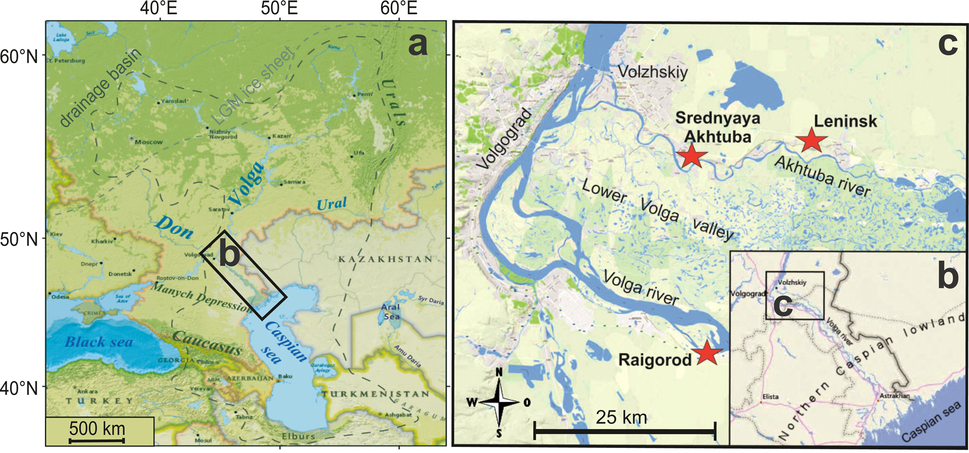
Figure 1. (color online) Map of the Caspian Sea region and surrounding areas with the study area located in the south of the Russian Plain (based on National Geographic World Map, Esri), the last glacial maximum ice sheet extent is depicted after Arkhipov et al. (Reference Arkhipov, Ehlers, Johnson and Wright1995) (a), in the Lower Volga region of the Northern Caspian lowland (b). The three study sites Srednyaya Akhtuba, Leninsk and Raigorod are marked with stars (c) (from Kurbanov et al., Reference Kurbanov, Murray, Yanina, Svistunov, Taratunina and Thompson2020).
The fluctuations of the Caspian Sea level and their driving factors are still to be resolved and understood. The extent to which these sea-level changes are related to Northern Hemisphere glacials/interglacials or regional climate changes is not yet well established, although many authors suggest a connection to glacial cycles (Chepalyga, Reference Chepalyga, Velichko, Wright and Baronsky1984; Varuschenko et al., Reference Varuschenko, Varuschenko and Klige1987; Velichko et al., Reference Velichko, Klimanov and Belyaev1987; Karpychev, Reference Karpychev1993). Many studies have focused on correlating transgressive and regressive oscillations with glaciation-deglaciation events occurring further north on the Russian Plain as well as the Siberian Plain (Milanovskiy, Reference Milanovskiy1932; Mirchink, Reference Mirchink1936; Nikolaev, Reference Nikolaev1953; Fedorov, Reference Fedorov1957, Reference Fedorov1978; Vasiliev, Reference Vasiliev1961, Reference Vasiliev, Alekseev and Tseitlin1982; Moskvitin, Reference Moskvitin1962; Markov et al., Reference Markov, Lazukov and Nikolaev1965; Kozhevnikov, Reference Kozhevnikov1971; Zubakov, Reference Zubakov1986; Rychagov, Reference Rychagov1997). One currently unexplained paradox is the occurrence of transgressions during phases of cold climate and glacial epochs when it is broadly agreed that conditions were drier in much of the region. Large transgressions are generally related to rapid water input due to deglaciation. In this context, the Volga River plays a significant role in understanding this relationship and several hypotheses try to explain this proposed link. A shift in the drainage systems of the Russian and Siberian plains is often considered as a potential factor, particularly via forced drainage of proglacial Russian Plain water into the Volga and similar events for rivers east of the Urals from the Siberian Plain, the latter case via the Aral Sea and Uzboy passage further to the east of the Caspian (Kvasov, Reference Kvasov1979; Grosswald, Reference Grosswald, Benito, Baker and Gregory1998; Mangerud et al., Reference Mangerud, Astakhov, Jacobsson and Svendsen2001) (Fig. 1a). In addition to the decaying Fennoscandian ice sheet as a potential water source (Kvasov, Reference Kvasov1979), increased precipitation in the Russian Plain (Volga catchment) causing more water runoff particularly during snow melt season, as well as the possibility of additional decreased evapotranspiration over the catchment area, are proposed as causes of transgressions (Sidorchuk et al., Reference Sidorchuk, Panin and Borisova2009). Local factors such as a decrease of evaporation over the Caspian Sea itself, or changes in the outflow from the Caspian, are also suggested (Yanko-Hombach and Kislov, Reference Yanko-Hombach and Kislov2018). Kislov et al. (Reference Kislov, Panin, Toropov and Yank-Hombach2014) hypothesized that the discharge of the Volga (followed by other rivers) as well as the precipitation-evaporation balance on the Russian Plain and in the local Caspian Sea region are the most important factors for the sea-level fluctuations. Although the actual source(s) of water are still unclear, most existing ideas lead to the conclusion that the main source of the additional water supply to the Caspian during cold transgressive phases lies on the Russian Plain, causing changes in Volga discharge (Yanko-Hombach and Kislov, Reference Yanko-Hombach and Kislov2018). Due to the relative proximity of the Caspian to the Black Sea, there is also a likely interaction between the two during some transgression stages via the Manych depression (e.g., Mangerud et al., Reference Mangerud, Astakhov, Jacobsson and Svendsen2001; Leonov et al., Reference Leonov, Lavrushin, Antipov, Spiridonova, Kuz'min, Jull, Burr, Jelinowska and Chalié2002), further complicating understanding the implications of sea-level history (Fig. 1a).
One obstacle towards understanding Caspian sea-level changes and its driving factors in the Quaternary is the interpretation of the origin and depositional environment of both marine and continental sediments. Records of environmental change from the Caspian region during the Caspian Sea fluctuations are needed to constrain the influence of local climate on the sea level cycles. Notably, there is a lack of paleoclimate information during regressive phases, when much of the Caspian region was sub-aerially exposed. In addition to the well-studied marine sediments that represent Caspian transgressive phases, considerable thicknesses of terrestrial deposits also comprise the Lower Volga sequences (e.g., Lebedeva et al., Reference Lebedeva, Makeev, Rusakov, Romanis, Yanina, Kurbanov, Kust and Varlamov2018). Periods of continental sedimentation under regressive phases are represented by fluvial sands as well as more silty, apparently sub-aerial deposits in the Lower Volga region. The origin and transport of these silty sediments, as well as their post-depositional modification, are controversial. While apparently displaying many characteristics of loess (in the general sense of accumulation of wind-blown terrestrial silts, sensu Muhs, Reference Muhs2013) (Lebedeva et al., Reference Lebedeva, Makeev, Rusakov, Romanis, Yanina, Kurbanov, Kust and Varlamov2018), the term “loess-like material” is used in many studies (Kolomiytsev, Reference Kolomiytsev1985; Shakhovets, Reference Shakhovets1987; Svitoch and Yanina, Reference Svitoch and Yanina1997; Lavrushin et al., Reference Lavrushin, Spiridonova, Tudryn, Chalie, Antipov, Kuralenko, Kurina and Tucholka2014). This careful way of addressing the material might derive from the common support for an in-situ loess formation theory by Russian scientists, one of the main paradigms of Russian loess research (e.g., Smalley et al., Reference Smalley, Marković, O'Hara-Dhand and Wynn2010, Reference Smalley, Marković and Svirčev2011). However, some authors are increasingly referring to these sediments as true wind-blown loess (Tudryn, Reference Tudryn, Chalié, Lavrushin, Antipov, Spiridonova, Lavrushin, Tucholka and Leroy2013; Lebedeva et al., Reference Lebedeva, Makeev, Rusakov, Romanis, Yanina, Kurbanov, Kust and Varlamov2018), although others still argue for an alternative genesis not involving aeolian dust transport, namely in situ silt particle formation from underlying sediments. In addition, Lavrushin et al. (Reference Lavrushin, Spiridonova, Tudryn, Chalie, Antipov, Kuralenko, Kurina and Tucholka2014) suggest re-working processes of slope sediments while instead Goretskiy (Reference Goretskiy1958) favours the idea of cryogenesis for the origin of this silt.
If the silt deposits of the Lower Volga sequences can be shown to be true aeolian loess, this material has great potential to contribute to a better understanding of past climate conditions and their evolution in the region. Loess is an excellent paleoclimate archive, containing a terrestrial record of past environmental change and near-source aeolian mineral dust (Muhs, Reference Muhs2013). In the Caspian basin, loess deposits can only be found along the Iranian coast (Khormali and Kehl., Reference Khormali and Kehl2011; Ghafarpour et al., Reference Ghafarpour, Khormali, Balsam, Karimi and Ayoubi2016) as well as, arguably, along the Lower Volga region where the combination of dry climate and low tectonic activity during the Quaternary made it possible for them to be preserved. Despite this, data from the Lower Volga region loess (or loess-like sediments) are scant in previous considerations of the paleoenvironmental evolution of the Caspian Sea region. Sediments from transgressive stages are described primarily in Russian literature, where past climate conditions are reconstructed based on marine fauna and sedimentological analyses (Fedorov, Reference Fedorov1978; Svitoch and Yanina, Reference Svitoch and Yanina1997). However, recent pedological investigations have begun to shed light on the environmental conditions during stages of continental sedimentation in the Lower Volga region, suggesting a cool and arid climate (Lebedeva et al., Reference Lebedeva, Makeev, Rusakov, Romanis, Yanina, Kurbanov, Kust and Varlamov2018). This investigation also points to local sources for the loess deposits, notably from marine sediments exposed during regression (Lebedeva et al., Reference Lebedeva, Makeev, Rusakov, Romanis, Yanina, Kurbanov, Kust and Varlamov2018). Presuming this silt material is indeed true loess then it will allow testing of some of the hypotheses of the Caspian sea-level fluctuations noted above, especially the importance of local versus regional climate factors.
Environmental magnetism is an effective way of deciphering continental climate records, particularly with regard to understanding the influence of local climate factors which are not often discussed in previous considerations of Caspian sea-level changes. Environmental magnetism can be used to constrain magnetic particle size, amount, type, and character, which allows understanding of syn- and post-depositional processes such as weathering, soil formation, and source change (Maher, Reference Maher2011).
In this paper, the first detailed mineral magnetic analysis of sediments in the Lower Volga region is presented and used to infer environmental changes and Caspian sea-level history at the time of loess or loess-like material deposition. The new magnetic data help constrain the nature and formation of this loess material, and thereby further inform the debate over the conflicting ideas of its genesis.
STUDY AREA
The Lower Volga and Russian Caspian Sea region
The level of the present day Caspian Sea water surface is 27 m below sea level and a major part of the exposed northern Caspian Sea coast lies in the southeastern extension of the Russian Plain (Fig. 1a). This area contains the estuary of the Volga River, which drains into the Caspian Sea forming a large delta (Fig. 1b).
South of the city of Volgograd, the Volga River changes from a narrow river to a wide braided fluvial system forming a large wetland area. This area extends around the main branch of the Volga and its major side branch, the Akhtuba River, often called the Volga-Akhtuba floodplain (Fig. 1c). The region is surrounded by a large lowland plain generally known as the Northern Caspian lowland, also referred to as the Lower Volga region. The characteristic environment is dominated at present by grass steppe vegetation with an average annual precipitation of 300–400 mm in its upper part (Sirotenko and Abashina, Reference Sirotenko and Abashina1992). Thus, a dry and continental climate currently controls the area. Regional-scale as well as local-scale wind systems can be important for the transport and dispersion of wind-blown dust in such areas dependent on whether distal or proximal dust deposits are formed (Pye, Reference Pye1995).
Quaternary geological setting and regional stratigraphy
In the late Pleistocene, the Caspian Sea experienced several transgression and regression phases (Fig. 2). These sea-level oscillations led to tens of meters differences in water level (e.g., Dolukhanov et al., Reference Dolukhanov, Chepalyga, Shkatova and Lavrentiev2009; Kislov et al., Reference Kislov, Panin, Toropov and Yank-Hombach2014) and the effect of these fluctuations can be clearly seen in the landscape of the flat northern coastline of the Caspian Sea in the present day Lower Volga region. Here, marine terraces dominate the geomorphology, representing alternating deposits of different marine facies intercalating with terrestrial sediments that were deposited during regressive stages (Yanina, Reference Yanina2014).
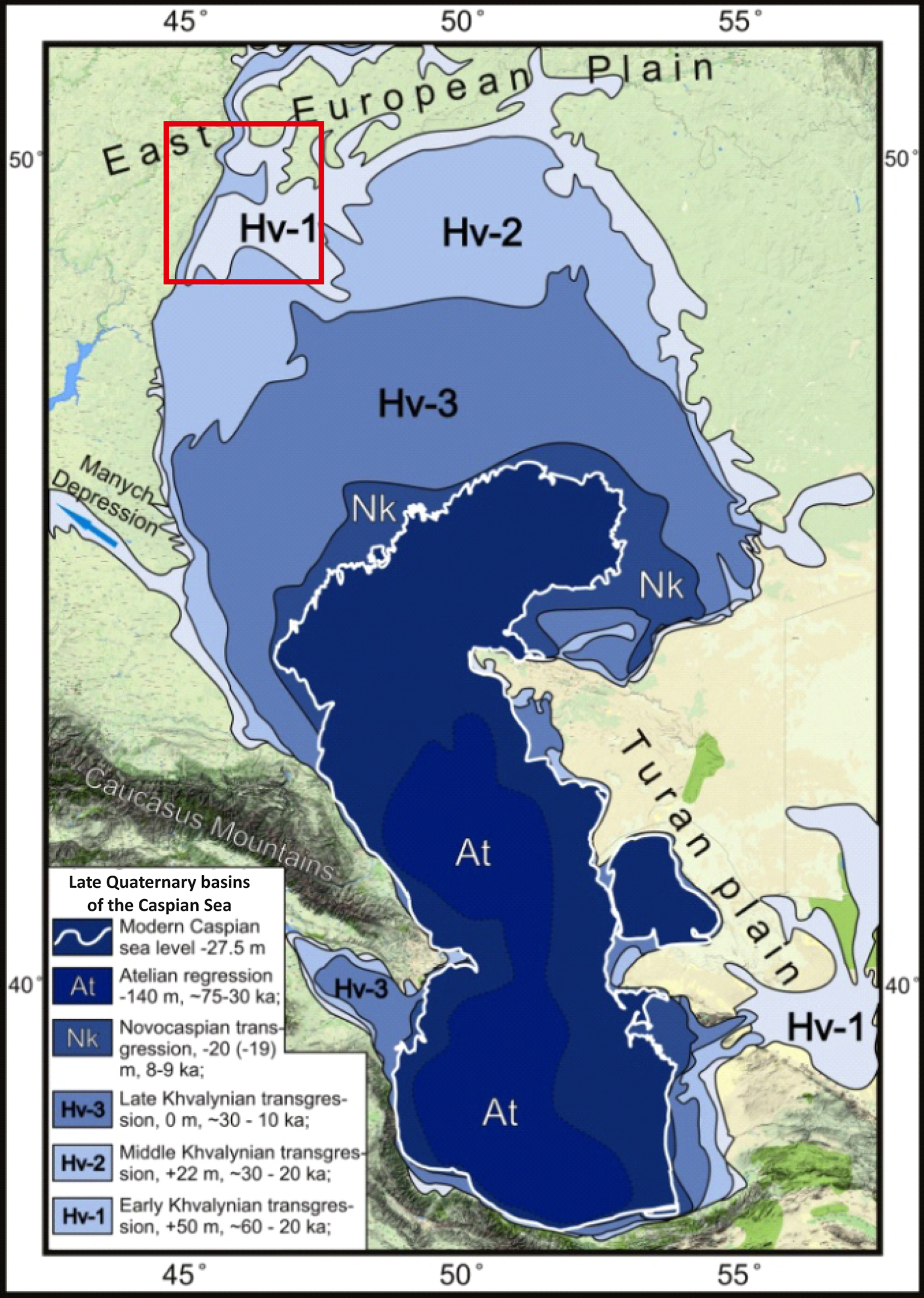
Figure 2. Caspian Sea level stands with elevations relative to modern global sea level during phases of transgression and regression in the Late Quaternary and in modern times (modified after Dolukhanov et al., Reference Dolukhanov, Chepalyga, Shkatova and Lavrentiev2009). The study area is marked by the red rectangle. Hv: Khvalynian; Nk: Novocaspian; At: Atelian. (For interpretation of the references to color in this figure legend, the reader is referred to the web version of this article.)
During the late Pleistocene, two major transgressions took place: the Khazarian and the Khvalynian. These are separated by the Atelian phase of regression (e.g., Krijgsman et al., Reference Krijgsman, Tesakov, Yanina, Lazarev, Danukalova, Van Baak and Agustí2019). Recently the possibility of a third transgressive stage, the Hyrcanian, has been elaborated on (Yanina et al., Reference Yanina, Svitoch, Kurbanov, Murray, Tkach and Sychev2017). Even though several different phases of sea level high and low stands in the late Quaternary Caspian Sea evolution can be identified and distinguished stratigraphically (Svitoch, Reference Svitoch and Svitoch1991; Rychagov, Reference Rychagov1997; Yanina, Reference Yanina2012), the age of certain events remains in question, as do the forcing mechanisms behind them (Table 1).
Table 1. Caspian Sea level evolution during the Late Pleistocene. (MIS = Marine Isotope Stage; m asl = meters above sea level)

The Khazarian Transgression
The Late Khazarian transgression is estimated to have reached sea-level stands from -10 to -5 m asl. (Varuschenko et al., Reference Varuschenko, Varuschenko and Klige1987), and the aerial extent of its surface area is estimated to have been slightly larger than the present Caspian Sea (Yanina, Reference Yanina2014). Its age, even though differing according to different authors and dating techniques, is broadly accepted to correlate with marine isotope stage (MIS) 5 (Tudryn et al., Reference Tudryn, Chalié, Lavrushin, Antipov, Spiridonova, Lavrushin, Tucholka and Leroy2013; Shkatova, Reference Shkatova2010). Late Khazarian deposits found in the region of the Lower Volga are typically represented by coastal sands with abundant marine fauna (Table 1). Marine biostratigraphy points towards stable and warm water conditions with low salinity in the upper Lower Volga region during MIS 5e (Shkatova, Reference Shkatova2010)
The Atelian Regression
Terrestrial deposits of the Atelian regression mark the end of the Khazarian in the Caspian Sea region (Svitoch, Reference Svitoch and Svitoch1991; Svitoch and Yanina, Reference Svitoch and Yanina1997). During the Atelian, the water level of the Caspian fell to -120 to -140 m asl, exposing large areas of the Caspian shelf. The base of the Atelian deposits, as described for the Lower Volga region, is represented by the Akhtuba sands. At many sites, cracks and wedges attributed to cryogenesis mark the lower boundary of the Akhtuba deposits (Goretskiy, Reference Goretskiy1958) and wedges can often be observed to penetrate into the underlying sediments, indicating periglacial conditions during their deposition (Goretskiy, Reference Goretskiy1958). The Atelian sediments overlying the Akhtuba sands are generally described as sandy loam and loam material up to 20 m thick, which stand as vertical walls (Moskvitin, Reference Moskvitin1962; Goretskiy, Reference Goretskiy1966; Sedaykin, Reference Sedaykin1988). In the Lower Volga sequences the material is referred to as loess-like (Table 1).
The occurrence of some stunted freshwater and continental mollusks as well as remains of mammals of the Upper Paleolithic fauna from about 35,000 to 10,000 years ago are reported from some sites in the Northern Caspian lowland (Yanina, Reference Yanina2014). This faunal assemblage is associated with cold and dry climate, so that the Atelian is correlated overall with MIS 4 and 3, representing a regional cold and arid time interval in the Caspian Sea region. In addition, up to four paleosol horizons are described within the Atelian deposits, while pollen records from the upper part of the Atelian deposits reflect a shift towards warmer climate (Yanina, Reference Yanina2014) (Table 1).
The Khvalynian Transgression
The Great Khvalynian represents the most extensive phase of transgression in the late Pleistocene. Sea level reached up to 50 m asl (Yanina, Reference Yanina2014), which means that the estuary of the Volga River into the Caspian Sea was located considerably further north than where the city of Volgograd is located today (Fig. 2). As the Kuma-Manych depression lies at an altitude of 27 m asl, interaction between the Caspian Sea and the Black Sea would have occurred, with drainage of the Caspian via the Black Sea to the global ocean (Mangerud et al., Reference Mangerud, Astakhov, Jacobsson and Svendsen2001; Leonov et al., Reference Leonov, Lavrushin, Antipov, Spiridonova, Kuz'min, Jull, Burr, Jelinowska and Chalié2002). Relict shoreline features of both the Early and Late Khvalynian phases can be found along all Caspian shorelines (Yanina, Reference Yanina2014). The Early Khvalynian transgressive stage is typically associated with the appearance of dark colored illite-rich sediments of fine grain size (Tudryn et al., Reference Tudryn, Leroy, Toucanne, Gibert-Brunet, Tucholka, Lavrushin, Dufaure, Miska and Bayon2016), commonly referred to as Chocolate clays (Makshaev and Svitoch, Reference Makshaev and Svitoch2016) (Table 1). Theories about the origin of the material suggest the clays represent either deep water facies formed during sea-level high stands (Svitoch and Makshaev, Reference Svitoch and Makshaev2015), material of ice sheet erosion from the Russian Plain (Makshaev and Svitoch, Reference Makshaev and Svitoch2016; Tudryn et al., Reference Tudryn, Leroy, Toucanne, Gibert-Brunet, Tucholka, Lavrushin, Dufaure, Miska and Bayon2016), or material from mudflows related to permafrost thawing (Moskvitin, Reference Moskvitin1962; Goretskiy, Reference Goretskiy1966). Badyukova (Reference Badyukova2007) in addition suggests that the Chocolate clays represent lagoon deposits. Khvalynian Chocolate clays on the river terraces in the Lower Volga region are found to be interbedded with thin layers of sand or silt (Tudryn at al., Reference Tudryn, Leroy, Toucanne, Gibert-Brunet, Tucholka, Lavrushin, Dufaure, Miska and Bayon2016). These sandy layers contain Khvalynian fauna (e.g., Makshaev and Svitoch, Reference Makshaev and Svitoch2016) (Table 1).
The timing of the Khvalynian transgression has not yet been fully agreed on. Nevertheless, it is broadly accepted that the Khvalynian can be subdivided into two major phases of transgression, potentially separated by a short regression named Enotaevka (e.g., Fedorov, Reference Fedorov1957, Reference Fedorov1978; Rychagov, Reference Rychagov1997). This subdivision is based on geomorphological features and corresponding sediments along the coastline (Dolukhanov et al., Reference Dolukhanov, Chepalyga, Shkatova and Lavrentiev2009) as well as biostratigraphic markers (Yanina, Reference Yanina2012). Absolute age estimates have also been obtained using a variety of methods (e.g., 14C, 230Th/234U). However, these are rather inconsistent, ranging from 70–10 ka, although many researchers favor a younger age for the Khvalynian (Svitoch et al., Reference Svitoch, Parunin and Yanina1994, Reference Svitoch, Selivanov and Yanina1998; Svitoch and Yanina, Reference Svitoch and Yanina1997, Arslanov et al., Reference Arslanov, Yanina, Chepalyga, Svitoch, Makshaev, Maksimov, Chernov, Tertychniy and Starikova2016) and the beginning of its first transgressive phase is widely believed to have occurred around 35 ka (Yanina, Reference Yanina2012) (Table 1). Thus, the Early Khvalynian transgression is generally agreed to have taken place during a cold glacial stage (Mamedov, Reference Mamedov1997). However, this timing contradicts the commonly accepted idea that transgressions in ice sheet water-fed water bodies are associated with melting of ice sheets, while regressions are believed to correspond to glaciation and ice advances. A key conclusion from this review is, therefore, that sea-level responses to wider climate/ice sheet forcing appear to be different for the Caspian during different time periods, potentially reflecting a range of causes for changes in sea level.
Sites and sampling
Information from three key sections from the upper Lower Volga region are presented in this study. The sites lie along the Lower Volga River braided fluvial system within the Volga-Akhtuba province (Fig. 1c). Srednyaya Akhtuba (SA) is located 30 km east of Volgograd on the east bank side of the Akhtuba River (48°42′1.44″N, 44°53′37.32″E). Just 30 km further east, Leninsk (LN) represents a natural outcrop in a dry gully towards the Akhtuba River (48°43′16.68″N, 45°9′33.12″E). Raigorod (RG) section lies on the west bank of the Volga River's main branch, 30 km south of SA, on the opposite bank of the upper Lower Volga River floodplain (48°25′52.68″N, 44°57′59.4″E). All sections were cleaned and made accessible before sampling in spring, 2017. Bulk samples were taken continuously at high resolution intervals of two centimeters throughout the whole section and for every stratigraphic unit. For the SA (18 m) and RG (21 m) sections, only samples from the outcrop's upper 14 m, comprising the Atelian loess-like deposits, were considered for environmental magnetic analyses. For LN (14 m, section 1) only samples from the loess-like part (6.7–14 m depth) of the sequence were used (Fig. 3).

Figure 3. (color online) Lithostratigraphic charts for the upper 14 m of Srednyaya Akhtuba, Raigorod and Leninsk sites. The ages for Srednyaya Akhtuba represent first OSL ages from Yanina et al. (Reference Yanina, Svitoch, Kurbanov, Murray, Tkach and Sychev2017) as well as unpublished data (Højsager, Reference Højsager2019). The boundaries of the Atelian deposits and between MIS 4 and MIS 3 for Raigorod and Leninsk are based on unpublished OSL dates.
METHODOLOGY
Mass dependent bulk magnetic susceptibility (χ, given in m3 kg−1) was calculated from the volume specific bulk magnetic susceptibility (κ, given in SI) measured by a MFK1-FA Kappabridge (AGICO; Pokorný et al., Reference Pokorný, Suza, Pokorný, Chlupáčová and Hrouda2006) at Uppsala University and the Schmidt Institute of Earth Physics RAS, Moscow. Measurements were carried out at a field amplitude of 200 A/m at room temperature using frequencies of 976 Hz and 15616 Hz, corresponding to low frequency (χlf) and high frequency (χhf) respectively, for samples taken every four cm at the studied profiles. Each sample was measured five times in a row before moving on to the next sample and the sample values presented here represent the mean of these data (Supplementary Table 1). Measurements at the two different frequencies allow calculation of frequency dependence of magnetic susceptibility (χfd, given in m3 kg−1 and χfd% given in %), an indicator for the presence of ultrafine superparamagnetic (SP) particles (Forster et al., Reference Forster, Evans and Heller1994). Due to its sensitivity to SP particles, χfd is often used to identify ultrafine-grained iron oxide formation due to pedogenesis, e.g., magnetite, maghemite, and hematite (Liu et al., Reference Liu, Deng, Torrent and Zhu2007; Maher, Reference Maher2011). Since SP grains fully contribute to χ at low frequency, the differences between the χlf of sediments and χlf of weathered horizons are often used as a proxy for soil formation (Liu et al., Reference Liu, Deng, Torrent and Zhu2007, Balsam et al., Reference Balsam, Ellwood, Ji, Williams, Long and El Hassani2011). However, the enhancement of χlf can be caused by increasing abundance of not only SP particles, but under certain conditions also by stable single domain (SSD), pseudo single domain (PSD), and multi domain (MD) grains. At the same time, paramagnetic minerals can contribute significantly to the χlf signal under certain conditions (Liu et al., Reference Liu, Deng, Torrent and Zhu2007; Nie et al., Reference Nie, King and Fang2007; Yang et al., Reference Yang, Hyodo, Zhang, Maeda, Yang, Wu and Li2013; Su et al., Reference Su, Nie, Luo, Li, Heermance and Garzione2019). This leads to two different models being proposed for controlling the χlf signal in loess, arising from two different sources. The most commonly known pedogenic enhancement model, which applies to Chinese loess (Heller and Evans, Reference Heller and Evans1995), describes the enhancement of χ due to pedogenic formation of SP grains during warm and moist climate periods (Liu et al., Reference Liu, Jackson, Banerjee, Maher, Deng, Pan and Zhu2004). The wind-vigour model instead suggests that a higher χ signal in deposits from colder periods is caused by stronger winds transporting coarser and denser iron oxide particles during these times (Evans, Reference Evans2001). Higher χ in loess than in paleosols can be observed for Alaskan and Siberian loess sites (Begét and Hawkins, Reference Begét and Hawkins1989; Chlachula et al., Reference Chlachula, Evans and Rutter1998). In Siberian loess, for example, increases in χ are shown to be primarily driven by wind dynamics leading to a coarsening of particles and increased detrital MD magnetite input (Evans and Heller, Reference Evans and Heller2003). Another explanation for χ in paleosols being lower than in the parent material is the chemical degradation of magnetite due to long-standing water-logged conditions. This model seems applicable for many paleosols in Russia, Poland and the west Ukraine (Babanin et al., Reference Babanin, Trukhin, Karpachevskiy, Ivanov and Morosov1995; Nawrocki et al., Reference Nawrocki, Wojcik and Bogucki1996).
Absolute χfd and its relative parameter χfd% are calculated using:


For very low χ values the range in accuracy of measurements might be bigger than the actual differences in susceptibility values at different frequencies (Pokorný et al., Reference Pokorný, Suza, Pokorný, Chlupáčová and Hrouda2006) so that the instrument's uncertainty makes the calculation of χfd meaningless. Where this appears to be the case (i.e., physically implausible negative frequency dependence), χfd is not presented.
While χfd is one possible method of checking the presence of SP grains and in particular is useful for indicating the ratio of ferromagnetic contributors with grain sizes close to the SP/SD boundary to the total assemblage, different magnetic parameters are needed to fully determine the domain state (and inferred grain size) of magnetic particles. Hysteresis measurements may provide such parameters (e.g., Tauxe et al. Reference Tauxe, Herbert, Shackleton and Kok1996; Tauxe, Reference Tauxe2010) helpful to gain further understanding of the nature of magnetic enhancement during pedogenesis, and to determine potential mixture of magnetic minerals (Forster and Heller, Reference Forster and Heller1997).
Magnetic hysteresis loops on pilot samples were recorded by measuring the samples with a Lake Shore Vibrating Sample Magnetometer (VSM; Ångström Laboratory, Uppsala University) at ambient temperature. Samples were prepared by compacting bulk sample material of known weight into gel caps, which were mounted between the poles of the electromagnet. Hysteresis measurements were made in fields up to 1 T, yielding parameters of saturation magnetization (Ms), saturation remanent magnetization (Mrs) and coercivity (Bc, also Hc). These parameters relevant to the ferromagnetic content are obtained by subtracting the paramagnetic contribution. Ms, Mrs and Bc values for each sample are listed in Supplementary Table 2. The squareness-coercive field plot (Tauxe et al., Reference Tauxe, Bertram and Seberino2002) allows the theoretical prediction of grain size and domain state of randomly oriented magnetic particles based on their squareness (Sq) as defined by the Mrs to Ms ratio and their Bc as defined by Stoner and Wohlfarth (Reference Stoner and Wohlfarth1948).
Anhysteretic remanent magnetization (ARM) was measured for pilot samples from each section. Oriented samples from LN were used for ARM analyses, while the loose sample material from SA and RG was compacted into plastic cubes of known volume and weight for ARM measurements. Measurements were performed with a 2 G Enterprises DC SQUID magnetometer (Uppsala University). Samples were placed in an alternating field (AF) of 100 mT with a superimposed direct current (DC) field of 0.05 mT. ARM was normalized to the DC bias field to obtain the magnetic susceptibility of ARM (κARM). Based on the κARM/κ ratios of natural and synthetic magnetites of different shapes and sizes, a simple model for magnetic granulometry to detect magnetic mineral grain size variations (King et al., Reference King, Banerjee and Marvin1983) was applied.
Along with the study of magnetic grain size, temperature dependent magnetic susceptibility (κT) was measured for a representative set of bulk samples to reveal the magnetic contributors in each lithology exposed at the sections. Measurements were done at a field strength of 200 A/m and a frequency of 976 Hz. The low temperature measurements were made by initially cooling down the sample to -192°C using liquid N and continuously measuring the susceptibility during warming to near 0°C. High temperature susceptibility measurements were made in an inert argon gas environment while warming from room temperature to 700°C. High temperature cooling curves represent measurements while temperature decreased back to room temperature.
To provide an initial quantitative estimate of past environments at the section, paleorainfall estimates were made based on χfd and χ following the model of Maher et al. (Reference Maher, Thompson and Zhou1994), with χB being the peak magnetic susceptibility in paleosols divided by the minimum magnetic susceptibility in loess, and χC the magnetic background susceptibility of loess:

As an alternative model, Maher et al. (Reference Maher, Alekseev and Alekseeva2002) uses χARM normalized by Mrs plotted against χlf and this is also presented here to test the applicability of Maher et al.'s (Reference Maher, Thompson and Zhou1994) model, which is limited to cases in which χfd and χlf are correlated.
RESULTS
Stratigraphy
All three sections represent similar stratigraphic sequences (Fig. 3) showing continental deposits such as sands and overlying loess-like sediments, covered by marine deposits. The upper 14 m of the three sections that are discussed here display the continental sand–loess-like sequence only for RG, although the same stratigraphic sequence is also present in SA and LN at a greater depth in the profile (SA: 17.6 m, LN: 16 m, section 2). Prominent cracks of 25–30 cm length infilled with the overlying material and penetrating into the underlying unit can be observed for the continentally derived sands of SA and RG sections (SA: ~8.5 m, RG: ~10 m; Fig. 3). SA differs from RG and LN by showing a clear erosional surface at the base of the continental sands and another thick loess sequence with paleosol horizons below, where by contrast dark clayey material can be found at other sites. Three weathered horizons apparently affected by pedogenesis can be identified visually within the upper continental deposits in SA and RG sections, as well as two in LN, even though they occur at very different depths. The visual characteristics are darker color, higher content of clay, and increased organic material. The pedogenetic horizons at SA are located at 4–5 m, 6.5–6.7 m and 7.4–7.7 m depth. RG shows signs of pedogenesis at 2–2.7 m, 3.3–4.2 m and 10–10.3 m. The pedogenic influenced horizons in LN are at 7.1–7.4 m and 13.4–14 m depth. Due to their mostly weak pedogenic development, these weathered layers are referred to as pedogenic horizons and not paleosols as commonly described in loess profiles. The pedogenic horizons are numbered in order from the top in each section without implying a stratigraphic correlation between horizons of the same name and number in the different profiles, as this has not been demonstrated. The uppermost of these three pedogenic levels is developed in loess-like material in all three sites, and so is the second at LN and RG. SA in contrast shows pedogenic level 2 developed in the sands. Level 3 also occurs in the sands at both, SA and also at RG.
The thickness of the loessic sequence (including pedogenic levels) overlying the sands is 8 meters for RG and LN and 2 m for SA. The boundary to the overlying marine sediments is clearly defined by an erosional surface in all three sections. The unconformity is partly very irregular, mostly dominated by sand on top of loess. The sand is horizontally bedded and is intensively interbedded with thin layers of dark brown Chocolate clay. The Chocolate clay layers become thicker higher up in the stratigraphic column until they are only interrupted by very thin sand layers showing cross-stratification. The sand layers contain distinct marine malacofauna and dark Mn-spots. On top of the marine sand-clay sequence modern soils, which are developed in a parent substrate of bioturbated marine clay and loess-like silt, complete the sections at all three sites (Lebedeva et al., Reference Lebedeva, Makeev, Rusakov, Romanis, Yanina, Kurbanov, Kust and Varlamov2018; Kurbanov et al., Reference Kurbanov, Murray, Yanina, Svistunov, Taratunina and Thompsonforthcoming).
The loess-like material of all three sections (SA: ~4.5–5.5 m and 8.5–12 m, RG: ~2–10 m, LN: ~7–14 m; Fig. 3) shows the same characteristics, being dominated by silt to very fine sand. The material is quite uniform in color and appearance; yellowish-brown, metastable, massive and open-structured. Initial grain size analyses show that the percentage of silt is approximately 70% and of sand approximately 20%. All continental deposits contain parts with signs of cryogenic processes and/or desiccation, showing clearly developed wedges and cracks. Other features observed in the continental sediments are carbonate and charcoal flecks, gypsum crystals, worm casts/root traces, and krotovina, which vary in their appearance at different stratigraphic levels in the sections (Fig. 3). Carbonate content ranges between 5 and 10% for calcite and less than 1% for dolomite on average.
Mineral magnetic analyses
The field observations and sedimentary analyses are complemented by the results from the different mineral magnetic analyses, which focus on the continental Atelian deposits of the sections.
χlf and χhf data show the same trend with depth in the profiles, with χhf values slightly offset to lower values. The deepest part of SA represents an exception, where χhf exceeds χlf (Fig. 4). The sands of the continental deposits have the lowest χ throughout the sections. The χ for the loess-like material of all three sections shows quite uniform and overall very low values, comparable to unaltered loess (6.72 x 10⁻⁸–2.02 x 10⁻⁷ m3 kg−1). Pedogenic horizons, intercalated in the loess-like units, are not clearly reflected in the χlf/χhf data (Fig. 4). The pedogenic levels that developed in the continental sands, however, show χ values (~1.3 x 10⁻⁷ m3 kg−1) higher than their parent material (~1–4 x 10⁻⁸ m3 kg−1) (Fig. 4). Compared to the clay and loess-like sediment however, these values are still low. The χfd curves show no strong correlation to stratigraphic variation with depth. For RG, a small enhancement in χfd can be observed for the two layers with pedogenesis at 2 m and 4 m. In the deepest part of the SA section, the overall very low values of χlf and χhf and limitations in measurement accuracy mentioned above limit the calculation and use of χfd in detecting ultrafine superparamagnetic minerals, and thus this is not presented (Fig. 4). The modern soils show the highest χ (χlf and χhf respectively) (up to 5 x 10⁻⁷ m3 kg−1) of all material and the boundary to the underlying marine sediments (SA: ~4 m, RG: ~2 m, LN: ~6.8 m) is clearly reflected in a shift towards lower χ values (~1.8 x 10⁻⁷ m3 kg−1) (Fig. 4).

Figure 4. Mass dependent and frequency dependent susceptibility curves for SA (a), RG (b), LN (c). The black points in the charts (for legend see Fig. 3) show the sample location of pilot samples for magnetic grain size and temperature dependent magnetic susceptibility analyses. (For interpretation of the references to color in this figure legend, the reader is referred to the web version of this article.)
Figure 5a shows χfd plotted against χlf for all loess-like and pedogenic units formed in these sediments for all three sites. A trend can be observed for samples from RG and to a minor extent also for SA. In the plots of Figure 5b–5d), loess-like and samples from pedogenic horizons for each section are presented separately. To allow a direct comparison between altered and unaltered material, only pedogenic horizons developed in loess-like parent material are displayed together with the data points from loess-like sequences.

Figure 5. (color online) χfd versus χlf plot for the loess-like-paleosol sequences of all three sites (a), as well as for Srednyaya Akhtuba (b), Raigorod (c) and Leninsk (d) respectively. Only pedogenic horizons with loess-like parent material are displayed.
Figure 6 shows the results of thermomagnetic experiments (κT) conducted on samples of loess-like material and pedogenic horizon material from the three sections. Heating curves show a gradual decrease in κT at low temperature for all samples. The normalized κT values reach zero with temperatures warming to 0°C. Sample LN-9-7 shows slightly different behavior and κT does not entirely drop to zero at 0°C. Samples LN-10-14, LN-11-7 and RG-177 show a sharp increase in κT at -150°C. During the high temperature experiments, all samples show decreasing susceptibility from around 520°C, with a sharp drop at 580°C. The κT of all samples decreases to nearly zero at 700°C. Another common feature is the small increase in κT between 280 and 400°C, clearly observable for all SA samples except SA-A-45 and most LN samples apart from LN-8-1 and LN-13-12, and for RG-193 and RG-255.

Figure 6. (color online) κT curves of the loess-like and pedogenic material pilot samples for SA (a), RG (b) and LN (c). The continuous lines represent heating curves, dashed lines show the cooling path of the heated samples. κT is presented as normalized by the highest value. The sample location in the sections is shown in Figure 4.
The determination of a material's magnetic grain size can be diagnostic for its formation conditions (Forster and Heller, Reference Forster and Heller1997). The squareness-coercivity field plot of Tauxe et al. (Reference Tauxe, Bertram and Seberino2002) indicates that the majority of samples fall into the defined area for MD grains (Fig. 7a). A few samples plot in the field for cubic single domain and superparamagnetic (CSD + SP) grains (Fig. 7a).

Figure 7. (color online) Magnetic domain state and inferred grain size determination after the models of Tauxe et al. (Reference Tauxe, Bertram and Seberino2002) (USD: uniaxial single domain (grains that can be magnetized in only one of two directions, thus showing uniaxial anisotropy); SP: super paramagnetic; MD: multi domain; L: length; W: width) (a); and King et al. (Reference King, Banerjee and Marvin1983) (b).
In the King plot (King et al., Reference King, Banerjee and Marvin1983) for relative grain size determination (Fig. 7b), all loess-like samples from RG are located in the plot region indicating magnetic mineral grain size between 0.2 and 1 μm. Most loess-like samples originating from LN as well as the sample from a pedogenic horizon fall close to the lines indicating grain sizes of 0.1 and 0.2 μm. The one LN loess-like sample showing lower κARM appears to contain coarser grains (Fig. 7b). The sample from a pedogenic horizon from SA indicates magnetic grain size slightly larger than 0.2 μm. The SA loess-like sample, however, shows significantly higher κARM and does not plot in the area of theoretical grain size determination. All samples with the exception of the RG sand sample and the SA loess-like sample suggest a similar magnetic grain size distribution (amount of magnetic mineral content) as indicated by their similar κARM/κ ratios.
Paleorainfall reconstruction
Paleoprecipitation calculations were performed to compare the Pleistocene Lower Volga region rainfall with the present regime and to put the data into context with other loess regions. Table 2 shows the paleorainfall reconstruction after Maher et al. (Reference Maher, Thompson and Zhou1994) from loess-like and pedogenic levels of the Lower Volga sections based on the equation of the linear trends from the plots of Figure 5. The results shown are calculated based on Equation 3 for each level. In the model for paleorainfall reconstruction of Maher et al. (Reference Maher, Alekseev and Alekseeva2002) all data points from the loess-like material plot in an area indicating very low annual precipitation (< 300mm) (Fig. 8).
Table 2. Estimated paleorainfall (mm a−1) for loess-like and pedogenic levels 1 to 3 (P1, P2, P3) for Srednyaya Akhtuba, Raigorod and Leninsk using the Maher et al. (Reference Maher, Thompson and Zhou1994) method, which does not outline uncertainties.


Figure 8. (color online) χARM/SIRM (given in meter per ampere) of loess-like samples from the Lower Volga sections plotted against χlf. Annual rainfall ranges and modern Russian steppe soils (Caspian Sea region and Caucasus) according to Maher et al. (Reference Maher, Alekseev and Alekseeva2002) are shown. The sample depth of the steppe soil samples from Maher et al. (Reference Maher, Alekseev and Alekseeva2002) is indicated (pm = parent material; described as well-mixed loess).
DISCUSSION
Chronostratigraphic subdivision of the profiles
The three Lower Volga sections show characteristic deposits from transgression and regression phases as well as a stratigraphic sequence similar to the typical regional stratigraphy of the Northern Caspian lowland (Fig. 3). This is particularly well displayed in the RG section, where classic Akhtuba deposits (correlated on the basis of diagnostic features such as the prominent cracks) underlie the loess-like material signaling a shift towards a drier depositional environment in the early Atelian (Fig. 3). Whereas LN comprises a similar sedimentary sequence to RG, SA differs more from the classic regional stratigraphic scheme. As described in the "Results” section, the key differences in the visual stratigraphy of SA can be found in the succession of the sand–loess-like sequence and connected to that, the presence of an additional erosional surface. A first introduction to the general stratigraphy of SA and a detailed soil stratigraphy is presented in Lebedeva et al. (Reference Lebedeva, Makeev, Rusakov, Romanis, Yanina, Kurbanov, Kust and Varlamov2018). Initial optically stimulated luminescence (OSL) dating results for SA suggest that the loess-like material corresponds in age to 62.1 ± 3.4 to 54.7 ± 3.2 ka between 12 and 8.5 m depth (Højsager, Reference Højsager2019). Kurbanov et al. (Reference Kurbanov, Murray, Yanina, Svistunov, Yarovaya, Taratunina, Butuzova, Semikolennykh, Thompson, Kurbanov, Yanina, Khavanskaya and Solodvnikov2018) dated the top of the loess-like sequence from SA below the erosional surface (8.5 m depth) to 48.7 ± 3.1 ka by OSL and this age is also supported by OSL dates published in Yanina et al. (Reference Yanina, Svitoch, Kurbanov, Murray, Tkach and Sychev2017). Considering these recent dating results, the occurrence of the continental sands in SA correlates with the beginning of the MIS 3 of the Atelian, contrasting with the regional stratigraphy and also with unpublished ages from RG and LN, where the same unit is dated to the beginning of MIS 4 and the onset of the Atelian regression. This suggests that the standard sedimentary sequence of the Atelian does not strictly apply over all the Northern Caspian lowland and that at SA, site-specific influences such as local river migration might be reflected. Initial OSL ages from the chocolate clays are 13.4 ± 0.7 to 16.1 ± 1.4 ka, depending on their stratigraphic depth and have been obtained from all three sections (Kurbanov et al., Reference Kurbanov, Murray, Yanina, Svistunov, Taratunina and Thompson2020). These dates overlap with a single radiocarbon age of 14.0 ± 2.0 ka from SA (Kurbanov et al., Reference Kurbanov, Murray, Yanina, Svistunov, Taratunina and Thompson2020). Existing OSL data of the continental deposits at RG and LN are currently unpublished, and the boundaries of the Atelian formation and MIS 3 and 4 are based on the established, yet unpublished, chronostratigraphy of the sections (Fig. 3).
Magnetic properties of the Atelian sediments
The loess-like material of all three sections shows very similar magnetic character in all magnetic experiments. The values for χlf, χhf and χfd% are within the same comparable range of 1.63 to 1.74 x 10⁻⁷ m3 kg−1 and 3–6% on average, indicating the significance of paramagnetic contributors to the bulk χ, similar to unaltered (aeolian) loess, observed in many loess sites (referenced in Table 3). The low temperature heating curves of the thermomagnetic experiments also display classic paramagnetic shapes (Fig 6). In contrast, paramagnetic behavior is not shown by the high temperature warming curves (Thompson and Oldfield, Reference Thompson and Oldfield1986).
Table 3. Comparison of published magnetic properties from classic loess regions from all over the world against measured values (average values ± standard deviation) from the Lower Volga sites.

Samples of rocks and soils showing purely paramagnetic behavior rarely show χlf values exceeding 1.0 x 10⁻⁷ m3 kg−1 or 5 x 10⁻⁴ SI for κT (Dearing, Reference Dearing1999). The χlf for the Lower Volga samples from all three sections and throughout the different lithological sequences ranges just above that value (Table 3). Considering that χlf values higher than 1.0 x 10⁻⁷ m3 kg−1 indicate the dominating influence of ferromagnetic contribution on the magnetic susceptibility signal and also that the thermomagnetic experiments (discussed later) clearly show the presence of ferromagnetic minerals, this suggests a mixed contribution of ferromagnetic and paramagnetic material to the bulk signal.
Compared to the loess-like units, the modern soil horizons in SA and RG contain more magnetic minerals than the other units and show the highest χ in each section (Fig. 4). This is likely to be driven by the neoformation of magnetic minerals by biochemical processes in the modern soil (Le Borgne, Reference Le Borgne1955; Mullins, Reference Mullins1977; Longworth et al., Reference Longworth, Becker, Thompson, Oldfield, Dearing and Rummery1979; Maher, Reference Maher1986, Reference Maher1998; Taylor et al., Reference Taylor, Maher and Self1987; Maher and Taylor, Reference Maher and Taylor1988). Sand samples showing lower χlf values than the other material indicate a smaller amount of magnetic minerals for the same volume of material and/or reflect a difference in composition (likely more diamagnetic particles) (Fig. 4). Generally, the main lithological units and boundaries between the different sediment deposits are well reflected by the mass dependent bulk magnetic susceptibility.
The magnetic behavior and domain state of magnetic minerals vary with temperature. By showing the variation of κ over a range of temperatures, specific minerals can be identified. The Curie temperature (TC) is diagnostic for each ferromagnetic mineral. It is typically characterized by a distinct decrease of κ during heating, which marks the transition to paramagnetic properties (Dunlop and Özdemir, Reference Dunlop and Özdemir1997; Evans and Heller, Reference Evans and Heller2003; Hrouda, Reference Hrouda2003; Tauxe, Reference Tauxe2010). The equivalent critical point temperature for antiferromagnetic minerals is the Néel temperature (TN) (Dearing, Reference Dearing1999). In the specific case of magnetite, a change in crystal structure results in a peak κ at -150°C, which indicates a crystallographic and electrical conductivity transition known as the Verwey transition (Verwey, Reference Verwey1939; Verwey and Haayman, Reference Verwey and Hayman1941).
The change of magnetic susceptibility values during thermal experiments indicates the following magnetic contributors in the analyzed samples: the most characteristic magnetic minerals in the loess-like samples are magnetite, titanomagnetite and maghemite. A sudden drop in κT, observed in all samples at 580°C, corresponds with the TC of magnetite (580°C). The Verwey transition of magnetite is clearly visible for a few samples from RG and LN, but not discernible for all of the specimens. However, the gradual decay of κT (starting around 500°C) observed in all curves before the drop at the TC of magnetite also indicates the presence of chemically inhomogeneous titanomagnetite (Lattard et al., Reference Lattard, Engelmann, Kontny and Sauerzapf2006) (Fig. 6). A higher Ti content in (titano-)magnetites will lower the TC (Evans and Heller, Reference Evans and Heller2003). Lagroix and Banerjee (Reference Lagroix and Banerjee2002) argue for a detrital origin of magnetite that hosts titanium, which does not appear due to pedogenic or weathering processes. The trend of κT enhancement between 280 and 400°C is likely to represent the reduction of maghemite to magnetite (Liu et al., Reference Liu, Shaw, Jiang, Bloemendal, Hesse, Rolph and Mao2010). This trend is present for several loess-like, clay, and sand samples observed in all sections. The trend observed for the modern soils of RG showing a decrease of κT between 300 and 400°C can be indicative for the decomposition of unstable maghemite due to its oxidation to hematite (Liu et al. Reference Liu, Deng, Yu, Torrent, Jackson, Banerjee and Zhu2005) (Fig. 6 and Supplementary Fig. A). However, even though possible, the formation of hematite in the inert argon atmosphere used in the experiment is unlikely. A TC of around 600°C shown by one RG clay sample may indicate stable maghemite (Liu et al., Reference Liu, Shaw, Jiang, Bloemendal, Hesse, Rolph and Mao2010) (Suppl. Fig. A). All marine clay samples indicate the presence of hematite due to their κT values remaining slightly positive after the decrease at the TC of magnetite (Supplementary Fig. A). However, the TN of hematite, visible in a decrease in κT at around 675°C (Dunlop and Özdemir, Reference Dunlop and Özdemir1997), cannot be clearly observed for any of the samples. Possibly this is related to the termination of heating at that temperature in the experiment but this is unlikely. Another reason could be the very common occurrence of impure hematite in natural environments causing a reduction of the TN due to Al substitution so that it possibly overlaps with the TC of magnetite (Cornell and Schwertmann, Reference Cornell and Schwertmann2003). A few loess-like samples from LN as well as most sand, clay, and modern soil samples from RG show signs of SD magnetite, as indicated by a gradual increase of κT from room temperature up to 280°C together with the TC of magnetite (Liu et al., Reference Liu, Deng, Yu, Torrent, Jackson, Banerjee and Zhu2005) (Fig. 6b and Supplementary Fig. A). In many samples, the susceptibility during cooling is much higher than the original κ, which is likely related to the neoformation of magnetite from clay minerals during heating (Ao et al., Reference Ao, Dekkers, Deng and Zhu2009). In sum, the temperature dependent susceptibility measurements show that besides others, magnetite is the main ferromagnetic mineral present in the samples, which strengthens the applicability of magnetic mineral grain size inference techniques, mostly theoretically developed for magnetite.
Frequency dependent magnetic susceptibility data (Fig. 5) can point towards the presence of SP and stable SD ferrimagnetic grains, in addition to MD contributions. The low χfd% in combination with the χlf values indicate a mixture of SP and coarser non-SP grains or SP grains < 0.005 μm (Dearing, Reference Dearing1999). The analyzed samples show χfd% between 3 and 6%, χfd of almost 0 and low χlf (Supplementary Table 1). A model introduced by Dearing et al. (Reference Dearing, Dann, Hay, Lees, Loveland, Maher and O'Grady1996) suggests that MD-dominated samples show relatively high χlf but zero χfd. χfd% <5% is inferred to be typical for samples containing stable SD grains or a very fine SP fraction (<0.005 μm). Samples dominated by SP grains show χfd% of 10% and more. In this context, the χfd and χfd% values of Lower Volga samples point towards the presence of MD and stable SD grains while the low χlf conflicts with Dearing et al.'s (Reference Dearing, Dann, Hay, Lees, Loveland, Maher and O'Grady1996) model. However, Dearing et al.'s (Reference Dearing, Dann, Hay, Lees, Loveland, Maher and O'Grady1996) conclusions result from measurements with an instrument other than the one used by us, limiting a direct comparison between values if not normalized.
A similar result can be inferred from the plots of χfd against χlf (Fig. 5), where the positive linear correlation between χlf and χfd for at least RG (strong positive correlation; R2=0.86) may indicate the presence of ultrafine SP grains produced by pedogenesis as it shows that the bulk susceptibility is increasing with increasing grade of magnetizability controlled by the contribution of the ultrafine superparamagnetic fraction represented by χfd (Forster et al., Reference Forster, Evans and Heller1994). By contrast, very weak correlation (R2=0.3), as can be observed for LN and SA, suggests very weak pedogenesis. Overall, despite the indication of a slight trend for certain horizons, no clear pedogenic enhancement can be inferred from the χlf-χfd correlation plots, which might signalize that fine-grained SD grains or a very fine SP fraction carry the χ signal in addition to MD grains. Terhorst et al. (Reference Terhorst, Appel and Werner2001) observe for loess in southwest Germany that fine-grained SD and PSD grains contribute significantly more to the χlf signal than generally assumed based on data from Chinese loess, reinforcing the range of models that may apply to loess from different regions.
The magnetic grain size determination by means of the squareness-coercivity field plot (Fig. 7a) (Tauxe et al., Reference Tauxe, Bertram and Seberino2002) shows that the domain state of the magnetic minerals present in the investigated loess-like and pedogenic samples are predominantly MD particles, trending towards uniaxial SD and SP grains. The presence of MD magnetite is also indicated by the trend of the thermomagnetic curves pointing towards an impurity with Ti content. Thus the combination of frequency dependent magnetic susceptibility and low field data (Figs 5 and 7) indicate MD contributors dominate over the additional presence of some SP and stable SD ferrimagnetic grains.
An even more specific magnetic mineral grain size estimation can be obtained using the ARM data (King et al., Reference King, Banerjee and Marvin1983). The dominant magnetic grain size determined by the King model ranges from 0.1 to 0.2 μm for most LN material and from 0.2 to 1 μm for most samples from SA and RG (Fig. 7b). At present, the reasons for this difference are unknown but might reflect a natural range of magnetic grain size variation for the loess-like sites at the Lower Volga. The overall linear correlation between κARM and κ for each site as observed in the King plot (Fig. 7b) indicates a constant grain size distribution for the magnetic contributors to the κARM and κ signal.
Loess-like sample SA-A-56 shows an anomalously high κARM value, which implies variation in the grain size of the magnetic minerals it contains. The sample plots in the MD field of the squareness coercivity field plot close to the boundary to the field of USD and SP grains, another hint that SA-A-56 contains more than just one magnetic grain size (Fig. 7a). For the other samples that plot in this same area, ARM data is unavailable and their grain size variation by means of their κARM value has not been estimated. Furthermore, the loess-like sample LN-32b (equals LN-8_1) shows a comparably high κ/κARM ratio, which suggests that its magnetic particles are coarser grained than other LN loess-like samples.
The origin of the Atelian silts
The debate on whether the silty loess-like continental material overlying the Akhtuba sands in the Lower Volga deposits is true loess (Muhs, Reference Muhs2013), carried by wind in its final stage of transport, or has rather formed in situ, has prevented the sites here from being fully utilized as climate records. Characterized by its appearance in the field, the material shows many properties associated with loess, such as its light yellowish-brown color, porosity, and massive structure. According to field and particle size observations, the material is dominated by silt particles with minor coarser or finer fractions. Another typical property is the homogenous appearance of the deposits without showing any bedding or stratification. Just as known for many classic loess areas (e.g., Li et al., Reference Li, Klik, Wu, Li, Poesen and Valentin2004), the Lower Volga sections also show a typical gulley morphology due to erosion by surface water. The steep walls of the outcrops, stable under dry conditions, are also characteristic for loess deposits (Rogers et al., Reference Rogers, Dijkstra and Smalley1994).
The similarities to loess would imply similarities in magnetic parameters as well, especially but not limited to magnetic grain size characteristics. Although the magnetic mineral concentration of loess (i.e., low field magnetic susceptibility) depends on the magnetic mineral composition of the source area of the dust, the effects of dust transport (e.g., dilution and mixing of the aerosol components during transport) means that the general χlf (κlf) of typical loess seems very similar over the European loess belt (ELB), the Central Asian loess region, and the Chinese loess plateau (CLP) (Table 3). Most of the loess units of various profiles from Eurasia show relatively low χlf (i.e., < 5 x 10⁻⁷ m3 kg−1) (Table 3). Unaltered loess from Siberian sites (referenced in Table 3) exceeds these values with a maximum of approximately 20 x 10−7 m3 kg−1 in some cases (discussed, for example, in Matasova et al., Reference Matasova, Petrovsky, Jordanova, Zykina and Kapicka2001). Generally, the χlf of loess is significantly lower than the χlf of paleosols due to magnetic enhancement by pedogenic processes (e.g., Evans, Reference Evans2001). There are some exceptions from Siberia (Kravchinsky et al., Reference Kravchinsky, Zykina and Zykin2008) and also from Alaskan loess (Lagroix and Banerjee, Reference Lagroix and Banerjee2004), for which the paleosol horizons show lower susceptibility values than the loess, which is related to the increasing detrital magnetic mineral input during glacial periods (wind-vigour enhancement model) and/or the specific characteristics of pedogenesis under cold, waterlogged, or permafrost conditions (Evans, Reference Evans2001).
The loess-like units at the study sites are characterized by low χfd% (3–4.7%) values that are within the range of unaltered loess and similar to the examples from the ELB, Central Asia, and the CLP (Table 3), even though as discussed above, a pedogenic model for magnetic enhancement may not be applicable for the Lower Volga material. It should be kept in mind that χfd% depends on several different factors and processes, so variations between sections and regions can be expected. However, true loess as a well-mixed sediment from various source rocks should never exceed a certain percentage of χfd% and cannot show similar high values as certain soils, which are dominated by primary or secondary ferromagnetic minerals (e.g., Maher, Reference Maher1986, Reference Maher1998). Maximum values for soils in England and Wales, for instance, are 12–14% (Dearing, Reference Dearing1999). The considerably lower χfd% values of the Lower Volga loess-like material are therefore similar to unaltered primary dust material comprising loess.
Coercivity and magnetization parameters obtained by hysteresis measurements can also serve as means for comparison with materials from various loess regions to test whether the studied units show characteristics in line with typical loess (Forster and Heller, Reference Forster and Heller1997). Based on the magnetic enhancement model of Forster and Heller (Reference Forster and Heller1997), which describes a material's enhanced mixture of magnetic minerals to show significantly higher susceptibility and lower Bc than the original mineral assemblage, loess from Paks (ELB), Karamaidan (Central Asia), and Luochuan (CLP) is characterized by higher Bc (Hc) values (~10–25 mT) compared to paleosol horizons (<10 mT). The samples from the Lower Volga successions show relatively low Bc (6.3–13.6 mT) in comparison to the examples provided by the model of Forster and Heller (Reference Forster and Heller1997). Despite their low value, the Lower Volga loess-like material is not a unique case (Table 3). Not all loess fits this model easily, as it implies a considerable proportion of high coercivity minerals in general for loess (e.g., hematite), which has not been identified in the Lower Volga or many other loess samples. The missing significant proportion of high coercivity minerals explains the lower Bc and the Lower Volga loess-like material indeed fits into the range of Bc values from many classic loess regions (Table 3). Loess units from these loess regions, including the ELB, Central Asia, and the CLP, are characterized by very similar values (Table 3) with the exception of the Nussloch loess (ELB), where relatively high Bc (30–50 mT) was measured (Taylor et al. Reference Taylor, Lagroix, Rousseau and Antoine2014). Finally, the Mrs/Ms ratio in the squareness-coercivity field plot (Fig. 7a) may be used to infer magnetic grain size via the domain state, with increasing Mrs/Ms ratio suggesting an increasing SD component (Dunlop, Reference Dunlop2002). Mrs/Ms of the Lower Volga loess-like deposits also falls into the range of Mrs/Ms values measured in other loess profiles from various loess regions (Table 3).
The overlap of Volga loess-like sediments with other classical loess sediments based on multiple magnetic parameters, combined with the field observations and initial sedimentological data, strongly suggests that the Volga material can be considered as true loess (sensu Muhs, Reference Muhs2013). This is supported by further observations from micromorphology and clay mineralogy at SA by Lebedeva et al. (Reference Lebedeva, Makeev, Rusakov, Romanis, Yanina, Kurbanov, Kust and Varlamov2018). Its formation due to direct airfall will therefore be assumed for the further discussion and the material termed as loess-like in this paper to this point will now be referred to as loess.
Late Pleistocene paleoenvironment in the Northern Caspian lowland
Paleoenvironmental indicators
Overall, the weak magnetic susceptibility of the Lower Volga loess points towards quite stable conditions of cool and dry climate restricting the in situ formation of magnetic minerals known from warm and moist environments (e.g., Maher, Reference Maher1986, Reference Maher1998; Maher and Taylor, Reference Maher and Taylor1988), particularly during MIS 4 (80–60 ka; Yanina et al., Reference Yanina, Svitoch, Kurbanov, Murray, Tkach and Sychev2017). To characterize some climatic components during the loess forming period in more detail, paleorainfall reconstructions were applied following Maher et al. (Reference Maher, Thompson and Zhou1994) (Table 2) and Maher et al. (Reference Maher, Alekseev and Alekseeva2002) (Fig. 8). The magnetic susceptibility based model of Maher et al. (Reference Maher, Thompson and Zhou1994) works well only for cases with strong correlation between χlf and χfd, which is not the case for the Volga loess (Fig. 5). This assumption becomes clear from the resulting estimates not showing conclusive differences between the loess and pedogenic material for the Lower Volga sections. Despite its inapplicability for climate inferences and the lack of specific indication for moister (drier) climate during times of soil formation (loess accumulation), the paleorainfall reconstruction after Maher et al. (Reference Maher, Thompson and Zhou1994) shows overall low annual precipitation suggesting dry environmental conditions during the Atelian. The model suggests that soil formation in the loess parent material at the Lower Volga sites did not affect the magnetic parameters driving the Maher et al. (Reference Maher, Thompson and Zhou1994) reconstructed paleorainfall signal since it does not yield clear differences for the amount of rainfall during the formation of loess and pedogenic material. This applies not only for SA and LN with their weak correlations between χlf and χfd (R2=0.3194; Figs 5b and 5d), but also for RG with its strong positive correlation of R2=0.8552 (Fig. 5c). The relatively low degree of pedogenic influence on the material of the Lower Volga sections and the apparent lack of applicability of the pedogenic mode of magnetic susceptibility signal acquisition, suggest that the paleorainfall estimates derived from the Maher et al. (Reference Maher, Thompson and Zhou1994) model might not be suitable to reconstruct the differences between rainfall during parent material accumulation and soil formation. These results are therefore complemented by the paleorainfall reconstruction based on the model of Maher et al. (Reference Maher, Alekseev and Alekseeva2002). This model is more generally applicable irrespective of mode of signal acquisition, and also suitable for unaltered material. Furthermore, it uses two different measured parameters where instead Maher et al. (Reference Maher, Thompson and Zhou1994) base their reconstruction on only one measured parameter as well as a derived value calculated from that. The results from the Maher et al. (Reference Maher, Alekseev and Alekseeva2002) method also indicate low annual precipitation of less than 300 mm a−1 for the loess from all of the three sections, similar to the Russian steppe loess parent material as described in the original study (Fig. 8). This also overlaps strongly with the amount of rainfall reconstructed applying the Maher et al. (Reference Maher, Thompson and Zhou1994) model. Similarly low paleoprecipitation was reconstructed during the deposition of loess (~MIS 4–10) from the ELB (220–340 mm/year, Panaiotu et al., Reference Panaiotu, Panaiotu, Grama and Necula2001; 340–400 mm/year, Bradák et al., Reference Bradák, Thamó-Bozsó, Kovács, Márton, Csillag and Horváth2011). Compared to this dry, possibly continental environment, the higher annual paleoprecipitation, recorded in the CLP (~MIS 2–15) (Liu et al., Reference Liu, Wei, Wang, Jin and Liu2016) indicates wetter glacial conditions in this monsoon region (590–800 mm/year for paleosols; 330–570 mm/year for loess).
Some variation in χfd% and some of the associated features (Fig. 4, and discussed in the “Results” section) appear distinct enough to imply a change of the magnetic characteristics within the loess sequence of the Lower Volga deposits, likely caused by a change of environmental conditions as the formation of iron oxides depends on climate (Maher et al., Reference Maher, Alekseev and Alekseeva2002). Both the type and grain size of iron oxides formed are controlled by different factors such as pH, oxidation rate, and Fe concentrations (Taylor et al., Reference Taylor, Maher and Self1987). χfd% variations can be found mostly in the loess deposits from MIS 3 (~40–25 ka; Yanina et al., Reference Yanina, Svitoch, Kurbanov, Murray, Tkach and Sychev2017) roughly corresponding to the sequences from 4–8.5 m in SA, 2–6.8 m in RG and 6.8–10 m in LN (Fig. 3) but also occur in the MIS 4 loess. For LN one such feature is given by the peak percentages of χfd% at 12.5 m depth. This increased χfd%, however, does not correlate with signs of pedogenesis in the section, instead some kind of reworking can be observed in the field for this part (e.g., cracks). The dissolution of fine-grained ferrimagnetic minerals by hydromorphic processes is reported from several areas in cool climates (Babanin et al., Reference Babanin, Trukhin, Karpachevskiy, Ivanov and Morosov1995; Nawrocki et al., Reference Nawrocki, Wojcik and Bogucki1996). Potentially, freeze-thaw processes of an active surface layer lead to vertical water flow rendering the downward transport of SP minerals possible. The peak χfd% at 12.5 m depth in LN could indicate the top of a preexisting permafrost layer, the impermeability of which prevented further vertical water flow. As such, SP minerals could possibly have accumulated at this level and lead to a higher χfd% signal than in the overlying horizon, where even a drop in χfd% can be observed, further supporting this idea. The occurrence of cryogenesis in MIS 4 deposits of the Northern Caspian lowland is well reported (Goretskiy, Reference Goretskiy1958) and evidence is also observed in the Lower Volga sections here (see Results section).
Also for RG, positive peaks in the χfd% curve can be observed. The most distinct one appears at around 4 m depth correlating to pedogenic level 2. Thermomagnetic analysis of samples from this layer indicate the presence of unstable maghemite, apparent in the κT enhancement between 280 and 400°C (e.g., Fig. 6b sample RG-147, RG-177 and RG-193). The occurrence of unstable maghemite in response to pedogenesis is well known for many loess areas, the Chinese Loess Plateau (Heller and Liu, Reference Heller and Liu1984; Liu et al., Reference Liu, Hesse and Rolph1999a; Maher, Reference Maher1998; Liu et al. Reference Liu, Deng, Yu, Torrent, Jackson, Banerjee and Zhu2005; Maher, Reference Maher2016), and also for Alaskan loess (Liu et al., Reference Liu, Hesse, Rolph and Begét1999b) and Siberian loess (Matasova et al., Reference Matasova, Petrovsky, Jordanova, Zykina and Kapicka2001; Zhu et al., Reference Zhu, Matasova, Kazansky, Zykina and Sun2003). Considering this established connection between pedogenesis and unstable maghemite appearance in loess, the maghemite in the relatively pristine loess of the Lower Volga is therefore likely derived from weak pedogenic processes. While coarse-grained maghemite of detrital sedimentary origin has been shown to be thermally very stable (Liu et al., Reference Liu, Banerjee, Jackson, Chen, Pan and Zhu2003), the inversion of maghemite to hematite at relatively low temperatures between 280 and 400°C in the Lower Volga samples (Fig. 6) supports its fine-grained character (Liu et al., Reference Liu, Deng, Yu, Torrent, Jackson, Banerjee and Zhu2005) and suggests its in-situ pedogenic formation. Ultrafine maghemite may form due to both the oxidation of ultrafine pedogenic magnetite (Chen et al., Reference Chen, Xie, Xu, Chen, Ji, Lu and Balsam2010) and/or as oxidized coatings on coarser lithogenic magnetite (Heller and Liu, Reference Heller and Liu1984). Fine-grained maghemite is also reported to form due to pedogenic weathering of Fe-bearing paramagnetic silicates and as such, to occur as inclusions in coarse-grained silicate minerals (Yang et al., Reference Yang, Hyodo, Zhang, Maeda, Yang, Wu and Li2013). This suggests that some weak pedogenic processes affected the loess in the Lower Volga region for some horizons, but was generally not sufficiently strong to cause neoformation of SP magnetite particles.
The plots of χfd against χlf suggest that magnetic susceptibility enhancement correlates with pedogenesis only for RG (Fig. 5). However, despite not being well developed due to the scatter of the loess samples, the plot for SA also shows that samples from the pedogenic horizons have higher χfd and χlf (Fig. 5b). Therefore, the appearance of weak pedogenesis in certain horizons of SA loess based on the field observations is also somewhat supported by the mineral magnetic data. Despite the apparent correlation between χlf and χfd for the pedogenic horizons of SA (Fig. 5b), the χfd% curve in the depth profile does not allow a distinct correlation between χfd% trends and pedogenic horizons (Fig. 4). Nevertheless, a slight enhancement of χfd% compared to their over- and underlying adjacent horizons is observed for some pedogenic levels in SA. Pedogenic level 1 shows a minor increase, pedogenic level 2 does not indicate enhancement of χfd% compared to the over- and underlying layer, while pedogenic level 3 reveals a more distinct enhancement in χfd%. In contrast, the χlf curve fully reflects the pedogenic levels (Fig. 4). This particularly applies for the pedogenic horizons developed in the sands (pedogenic levels 2 and 3). Compared to its sandy parent material, these two pedogenic levels clearly show higher χlf values. One reason why pedogenic horizons might show an increase in χlf without showing any increase in χfd% could be the influence of hydromorphic conditions on the magnetic minerals or soil truncation. Waterlogging can lead to the preferential dissolution of SD and small PSD particles before affecting MD grains (Taylor et al., Reference Taylor, Lagroix, Rousseau and Antoine2014). In fact, the available magnetic grain size analyses indicate the dominance of MD grains (Fig. 7) and only a few loess samples from LN indicate presence of SD magnetite (Fig. 6). However, the χfd%/χlf /χhf depth curves and the χfd versus χlf diagram indicate the presence of some SP grains for pedogenic levels at SA to some degree (Figs. 4a and 5b). For the sand-paleosol sequence of SA (ca. 5.5–8.5 m) no magnetic grain size and thermomagnetic data is available but in situ formed maghemite was detected in pilot samples from MIS 3 pedogenic layers developed in the loess of RG and LN, also indicating mineral alteration induced by weak pedogenesis during a phase of less arid climate. Increased abundance of pedogenic maghemite with increased rainfall has also been shown by Gao et al. (Reference Gao, Hao, Old, Bloemendal and Deng2019) for the monsoon-affected CLP.
It should be considered that the loess was covered by a marine transgression for several ka (~10 ka, Kurbanov et al., Reference Kurbanov, Murray, Yanina, Svistunov, Taratunina and Thompson2020), as the marine sand and clay overlying the loess deposits clearly reveal. A comparable setting is not known from any other loess site and appears to be unique for the Lower Volga profiles. The influence of shallow marine water cover on the magnetic properties of continental material and coincident diagenetic effects are therefore not discussed in the literature. Nevertheless, magnetic properties of marine material, also in respect to paleoclimate, are well studied (e.g., Arai et al., Reference Arai, Sakai and Konishi1997; Kissel et al., Reference Kissel, Laj, Labeyrie, Dokken, Voelker and Blamart1999; Oldfield et al., Reference Oldfield, Asioli, Accorsi, Mercuri, Juggins, Langone and Rolph2003; Kumar et al., Reference Kumar, Purnachandra, Patil, Kessarkar and Thamban2005). Very low concentrations of fine-grained ferrimagnetic minerals or even no χfd signal at all can be observed when fine-grained ferrimagnetic iron oxides are subject to reduction, leading to their dissolution. This is caused by oxygen depletion as a result of the decomposition of organic matter (e.g., Grimley and Arruda, Reference Grimley and Arruda2007). Despite the χfd signal of pedogenic horizons being very low in the Lower Volga profiles, no marine sediments characteristic of strongly reducing conditions, which could have affected the underlying continental material, seem to have deposited during the marine transgression. This can also be inferred from the thermomagnetic data, which does not show any signs of ferrimagnetic greigite, which typically forms under reducing conditions (Mann et al., Reference Mann, Sparks, Frankel, Bazylinski and Jannasch1990; Horng, Reference Horng2018; Rudmin et al., Reference Rudmin, Roberts, Horng, Mazurov, Savinova, Ruban, Kashapov and Veklich2018) (Fig. 6). We therefore infer that the water depth of a few tens of meters was too shallow and the water column too well mixed throughout to cause significant degradation of organic matter and a reducing environment. In addition, the presence of sea water would most likely have affected only the uppermost meter(s) of the continental deposits by infiltrating and saturating the substrate so any effect on and diagenesis of magnetic minerals would probably only be visible for pedogenic horizon 1 in each profile. These soils do not display any χfd trends significantly different to the other pedogenic horizons but show rather low χfd without clear enhancement. Different from some hydromorphic conditions that have been proposed to possibly wash out ultra-fine-grained SP particles from the substrate (e.g., Taylor et al., Reference Taylor, Lagroix, Rousseau and Antoine2014), a marine environment does not imply vertical water movement in the covered sediment, so that a leach-out of fine magnetic material does not seem very plausible. To a certain extent pore water movement would occur since loess is a rather porous and permeable material. This could lead to the solution of carbonates. After the marine regression and desiccation of the deposits, carbonate-enriched solutions might have been retained in the pores of the loess leading to the formation of carbonate concretions (Haldar and Tišljar, Reference Haldar and Tišljar2014). Indeed, carbonate flecks as well as gypsum crystals appear in the uppermost loess and pedogenic horizons below the erosional surface, potentially indicating products of marine infiltration and subsequent evaporation (Fig. 3). However, the overall carbonate content of the profiles does not indicate significant leaching in connection with the marine transgression. Thus, there is no clear evidence that marine transgression would have significantly altered the magnetic properties of the buried loess material, although this topic is relatively new in magnetic research due to the unique situation of the Lower Volga loess.
Paleoenvironmental history
Field observations strengthen the inferences from the mineral magnetic data of general cold aridity in the Northern Caspian lowland over the time period of Atelian loess deposition. The sections comprise loess, which accumulated approximately four meter thick deposits over 20 ka (Højsager, Reference Højsager2019). The weak pedogenic levels are developed mainly in the upper continental deposits (MIS 3) of the sites. This supports the observations from loess sections in the Azov Sea region that pedogenesis occurs during MIS 3 (Liang et al., Reference Liang, Yang, Velichko, Zeng, Shi, Wang, He, Chen and Chen2016). Neither pollen nor continental gastropods are found in the loess sequences, also potentially suggesting dry and cool conditions probably unfavorable for significant growth of vegetation and the propagation of gastropods. Charcoal flecks are present to a minor extent and lead to the interpretation that the late Quaternary landscape of the Lower Volga was comprised of dry steppe vegetation occasionally affected by fire, as is the case today. The paleorainfall reconstructions for the Atelian support this idea of a semi-arid, continental steppe environment comparable to the one of the modern Lower Volga region, showing annual precipitation of < 300 mm. Similar suggestions come from Velichko et al. (Reference Velichko, Catto, Yu Kononov, Morozova, Novenko, Panin, Ryskov and Semenov2009) and others, and the low χfd of modern soils in the Northern Caspian lowland (Maher et al., Reference Maher, Alekseev and Alekseeva2002) are comparable to the Atelian paleosols in the Lower Volga sections. However, there is no active loess formation in the Lower Volga region today (Maher et al., Reference Maher, Alekseev and Alekseeva2002), indicating greater dustiness during the Atelian. Cooler climate conditions during the Atelian than today can also be inferred from the signs of cryogenesis found in the Lower Volga sequences (Fig 3).
The accumulation and diagenesis of loess in the region correlates with related episodes of cool and dry climate and loess deposition in many regions in the world (e.g. Muhs, Reference Muhs2013). The period of cold aridity in the Lower Volga represented by the loess sequences can be clearly identified and distinguished from the overlying marine deposits by field observation and magnetic susceptibility data (Fig. 4), implying a sea-level rise of the Caspian following the cool and arid regressive stage. The first OSL dating results from SA (Yanina et al., Reference Yanina, Svitoch, Kurbanov, Murray, Tkach and Sychev2017, and unpublished data) verify that the loess and clays were deposited from the time period of the Atelian regression (~27–80 ka, MIS 4–3) and Khvalynian transgression, respectively (~23–13 ka, MIS 2).
The χfd data from loess representing MIS 4 deposits (below the erosional surface at ~8.5 m in SA, lower loess parts in RG and LN; Fig. 3) show more stable environmental conditions than during the MIS 3 of the Atelian (~4–8.5 m in SA, upper loess parts in RG and LN, Fig. 3) (Fig. 4). Paleoclimate reconstructions from paleosol-loess records in the neighboring Azov Sea region suggest MIS 4 to be the coldest phase of the last glaciation in the region (Liang et al., Reference Liang, Yang, Velichko, Zeng, Shi, Wang, He, Chen and Chen2016) with stronger wind intensities than during the other stages (Novothny et al., Reference Novothny, Frechen, Horváth, Wacha and Rolf2011).
Overall, the chronostratigraphic and mineral magnetics data show that pedogenesis took place in the Lower Volga loess deposits during the late stage of the generally cool and dry regressive phase of the Atelian, corresponding to MIS 3. We describe up to three pedogenic levels for the MIS 3 Atelian loess part of RG and LN and the loess/sand sequence of SA. While not immediately apparent in the bulk magnetic susceptibility data, all of them show specific magnetic properties related to weak soil formation, which signals shifts towards less arid and/or warmer climate during the times when the pedogenic horizons developed. The conditions during these climate excursions might still have been rather cool but with likely increased and possibly seasonal rainfall. This is indicated by the presence of magnetite and maghemite and absence of hematite and goethite in samples from these horizons, the latter of which forms preferably under warm and dry conditions (Taylor et al., Reference Taylor, Maher and Self1987; Schwertmann, Reference Schwertmann, Stucki, Goodman and Schwertmann1988). The generation of magnetite instead is favored by intermittent wetting and drying of the ground (Maher et al., Reference Maher, Alekseev and Alekseeva2002). Possibly this increase in humidity came along with a certain increase in temperature. Magnetic proxies are potentially affected by both precipitation and temperature, which can make it difficult to estimate the crucial environmental driver (Nie et al., Reference Nie, Stevens, Song, King, Zhang, Ji, Gong and Cares2014). For regions in which a coupled increase/decrease of temperature and precipitation applies at certain intervals, magnetic proxies may be relatively straightforward to interpret but become less accurate whenever a potentially different trend of the two environmental factors has to be considered (Nie et al., Reference Nie, Stevens, Song, King, Zhang, Ji, Gong and Cares2014). For the cold and dry environment in the Lower Volga region during the Atelian it is hard to say whether it was temperature or precipitation or both that affected the magnetic proxies. Even though magnetic minerals indicative for warm and moist climate are not distinctly apparent and pedogenesis is developed more weakly than would be expected under the influence of warm temperatures and humidity, a small rise in both cannot be excluded. Indeed, supporting this is field evidence that the MIS 3 soils, in contrast to the MIS 4 deposits, are not affected by cryogenesis. The most humid and/or warmest period might have taken place during the formation of RG pedogenic level 2, where χfd% data shows the most distinct signs for ultrafine SP grains in the RG section. As far as the pedogenic levels can be put in relation with absolute ages at this point, this period might have occurred around 30 ka.
As shown in the discussion above, the data presented in this work indicate that the Atelian regression in the Northern Caspian lowland coincided with generally cold and arid climatic conditions punctuated by slightly increased humidity and/or temperatures during its later phase. This could imply a certain local-regional climatic influence on the low water level of the Caspian Sea during that period and on its rise during MIS 3. Especially when considering the enhanced soil formation during MIS 3 compared to MIS 4 as sign for a change to wetter climate and potentially higher precipitation in the region, the shift from a regressive to a transgressive regime as forced by local climate appears plausible. This would imply that the Caspian sea level might therefore not only be controlled by changes in precipitation or water run-off due to ice melting in relevant river catchment areas on the Russian and Siberian Plains, but could also be a function of local climate change. However, the reconstructions presented here show generally cooler climate during the Atelian than today, but with potentially similar precipitation amounts. Lower evaporation rates under a cooler climate would imply that with the same amount of precipitation sea level ought to have risen over this period. Since the Atelian is characterized by low sea-level stands, this mismatch implies that external factors must have been the dominant control on the Caspian water level over that interval. While overestimates of precipitation from our reconstructions are possible, the scale of the regression and the likely lowering of temperature in the region as witnessed from cryogenic features still demand an alternative explanation for the sea-level drop. It is therefore very likely that river discharge of the Volga and other rivers is mainly responsible for Caspian sea-level change during the cold climate phases of the Pleistocene, and that reductions in discharge of these rivers during the earlier part of the last glaciation drove the Atelian Caspian sea-level fall. However, sea-level rise during MIS 3 did most likely coincide with increased temperature and humidity in the region. Increased local precipitation during this late stage of the Atelian might therefore have had an additional effect on the onset of the Khvalynian transgression, even if this was ultimately mainly forced by ice sheet melting and Volga discharge.
CONCLUSION
This first detailed magnetic study for sections in the Lower Volga region shows that χlf distinguishes well between layers of different sedimentary material in the sections. The material characteristics obtained from the magnetic investigations support those from field observations, showing that the loess-like material can be defined as true aeolian loess, in the sense of a primary air fall terrestrial dust deposit. This further is supported by the comparison of Lower Volga loess and typical loess regions in Europe, Central Asia, and China, all showing similar magnetic characteristics.
The χfd% data shows that the loess of the Lower Volga sections mostly forms a homogeneous unit, implying stable cool and arid conditions particularly during the MIS 4 of the Atelian regression. However, together with the applied rock and environmental magnetic methods (magnetic grain size determination and κT), small shifts in the paleoenvironment particularly in the upper part of the loess (MIS 3) are evident. A combination of the χfd, hysteresis, ARM, and κT data indicates the occurrence of weak pedogenesis in the loess during potentially more humid and warmer periods. At least three shifts towards more moist/warm environmental conditions can be determined from the Lower Volga loess deposits. The most humid/warm climate might have occurred during the formation of pedogenic level 2 in the RG section around 30 ka.
Paleorainfall reconstructions indicate low precipitation of approximately < 300 mm a−1 during the depositional period, including during the periods when pedogenesis took place. This suggests a semi-arid environment with dry steppe vegetation similar to today's Lower Volga region. This combined with the locally cold periglacial climate ought to have forced higher sea levels of the Caspian during the Atelian relative to today, if local-regional climate were the dominant control on sea level. As such, the data here rather support the idea that changes in river discharge due to decreased precipitation or increased glaciation on the Russian and Siberian Plains is the main reason for the Caspian Sea low stand during the cold Atelian regression, with reduced river discharge into the Caspian. Nevertheless, the signs for potentially increased humidity during MIS 3 suggest local-regional climate changes to be a potential additional driver of later sea-level oscillations to some extent.
ACKNOWLEDGMENTS
We are grateful to Tamara Yanina for her help in organizing the field work in the Lower Volga region. Thanks go also to Elena Degtyareva and Vladimir Pavlov from the Schmidt Institute of Earth Physics RAS for providing their lab facilities and support with instrument application. Acknowledgement goes also to Steffen Wiers for his Uppsala University in-house written software “Fika” to operate the SQUID magnetometer and ready technical support. The Swedish Research Council is gratefully acknowledged for funding to Thomas Stevens for part of this project (2017-03888). The work of Redzhep Kurbanov was supported by the Russian Science Foundation (grant 19-77-10077). Sofya Yarovaya was supported by the Russian Foundation for Basic Research (grant 18-00-00470). Balázs Bradák acknowledges the financial support of project BU235P18 (Junta de Castilla y Leon, Spain) and the European Regional Development Fund.
SUPPLEMENTARY MATERIAL
The supplementary material for this article can be found at https://doi.org/10.1017/qua.2020.73
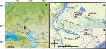


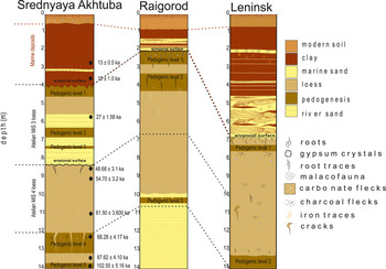
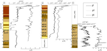
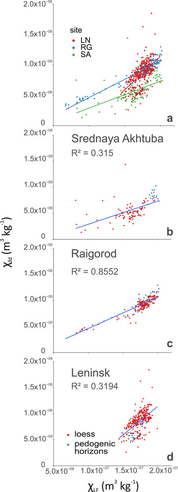
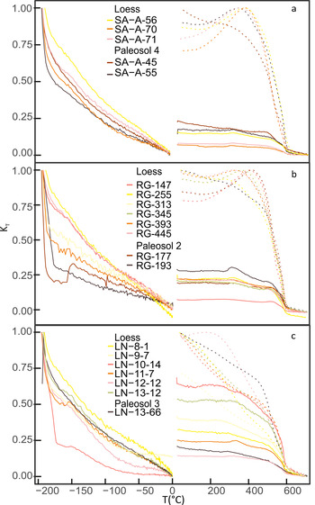
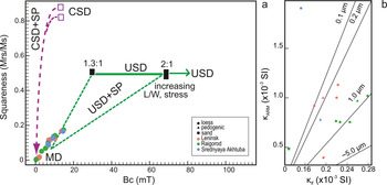


 Open access