


1. Introduction
In a robot control system, an accurate dynamic model of the robot is fundamentally important for accurate and stable control [Reference Gaz, Cognetti, Oliva, Giordano and De Luca1]. This is true for all kinds of robots, such as industrial robots, humanoid robots, medical robots, soft robots, and exoskeletons. However, accurate dynamic models only exist in theory but not in practice, since various uncertainties can be residing in the dynamic model inevitably. Examples of such uncertainties are joint friction, inaccurate center of mass location and link weight, extra payload, and robot-environment interaction [Reference Gaz, Cognetti, Oliva, Giordano and De Luca1]. Therefore, it is a fundamental topic for estimating and compensating for uncertainties in the field of robot control.
Many methods have been developed for estimating dynamic uncertainties thus eliminating their effects on robot dynamics. Disturbance observer is a main solution that can observe the dynamic uncertainties in an online manner, thus making compensation accordingly when necessary. Besides the observers, many learning techniques have been also applied for disturbance estimation and compensation, such as using feedforward neural network (NN) [Reference Panwar and Sukavanam2–Reference Liu, Wang and Wang4], and nonlinear autoregressive network with exogenous inputs (NARX) [Reference Sharifi, Mehr, Mushahwar and Tavakoli5]. Since the learning-based methods for disturbance estimation are beyond the scope of this paper, they will not be introduced here.
A variety of observers have been developed [Reference Radke and Gao6, Reference Chen, Yang, Guo and Li7], but not all of them can be implemented into a robotic system. The typical observers selected in this paper are identified according to the following procedures. First, a list of observers is collected based on three recent review papers [Reference Haddadin, De Luca and Albu-Schäffer8–Reference Chien, Wang and Cheng10] and one research paper [Reference Hu and Xiong11]. Then, the following two rules are applied: (a) the observer is applicable in practice in a physical robotic system and (b) the observer is independent of the controllers, that is, not relying on a specific controller. Finally, five typical observers are identified, including generalized momentum observer (GMO) [Reference Haddadin, De Luca and Albu-Schäffer8], joint velocity observer (JVOB) [Reference Haddadin, De Luca and Albu-Schäffer8], extended state observer (ESO) [Reference Sebastian, Li, Crocher, Kremers, Tan and Oetomo12], nonlinear disturbance observer (NDOB) [Reference Mohammadi, Tavakoli, Marquez and Hashemzadeh13], and disturbance Kalman filter (DKF) method [Reference Liu, Wang and Wang4, Reference Hu and Xiong11]. In this paper, we will focus on surveying these five typical types of disturbance observers, that is, GMO, JVOB, ESO, NDOB, and DKF. For the ESO, three of its variants are presented, including the original ESO (ESO.orig), a modified ESO (ESO.modi), and an improved ESO (ESO.impr).
Generalized momentum observer (GMO), also known as classic first-order momentum observer, is originally proposed for actuator fault detection and isolation, aiming to avoid joint acceleration measurements and inverse of the robot inertia matrix in the control system [Reference De Luca and Mattone14, Reference De Luca and Mattone15]. Note that in practice, measuring accelerations is usually avoided due to their high price or installation size restrictions. Furthermore, obtaining accelerations via numerical differentiation of velocity or position is not preferred since it will introduce noise into the system and thus may affect the system’s stability [Reference Haddadin, De Luca and Albu-Schäffer8]. The inverse of the robot inertia matrix can increase the computational load on the system. Besides not requiring the accelerations and inverse of inertia matrix, the GMO also has the advantage of being simple, compact, and easy to implement [Reference Zhang and Liang16], all of which make it one of the most commonly used observers. It is usually used as a benchmark for comparison when designing new observers [Reference Liu, Wang and Wang4, Reference Hu and Xiong11, Reference Garofalo, Mansfeld, Jankowski and Ott17].
Joint velocity observer (JVOB) is a similar observer to the GMO in terms of the procedures of derivation and the final expression, but the inversion of the robot inertia matrix is needed [Reference Haddadin, De Luca and Albu-Schäffer8]. The JVOB is derived based on the acceleration expressed by the robot dynamics, then the integration of the acceleration is taken as an estimate of the velocity where the true velocity is assumed to be known. Therefore, the JVOB is a reduced (first-order) observer with a reduced state of dimension
 $n$
, where
$n$
, where
 $n$
is the number of the generalized coordinates of the robot.
$n$
is the number of the generalized coordinates of the robot.
Extended state observer (ESO) was originally proposed by Han in the 1990s, and it is considered as the critical part of active disturbance rejection control (ADRC) which is developed to estimate the lumped uncertainties including both unknown dynamic uncertainties and external disturbances [Reference Han18, Reference Han19]. For a specific survey on ADRC and ESO, please refer to ref. [Reference Huang and Xue20]. In another historical survey on observers in 2006 [Reference Radke and Gao6], ESO has been viewed as an indicator of an initial shift of design methodology from modern estimators (e.g., Kalman Filter) to disturbance estimators (e.g., ESO). The ESO employs a simple canonical form which is considered as a practical design; thus, it receives many applications in different fields, such as power converters, web tension, and bio-mechanics [Reference Radke and Gao6]. In the field of robot control, various variations of ESO have been developed in different application scenarios such as collision detection [Reference Ren, Dong, Wu and Chen21] and time-varying interaction force estimation [Reference Sebastian, Li, Crocher, Kremers, Tan and Oetomo12].
Nonlinear disturbance observer (NDOB) is originally proposed by Chen, which is considered to overcome the shortcomings of linear disturbance observer that is designed or analyzed by linear system techniques [Reference Chen, Ballance, Gawthrop and O’Reilly22]. Although this version of NDOB was developed for constant disturbances in theory, it also revealed satisfactory performance on estimating time-varying disturbances like friction. However, it is merely used for planar robots with revolute joints. To solve this problem, Mohammadi et al. [Reference Mohammadi, Tavakoli, Marquez and Hashemzadeh13] proposed a general framework for NDOB by unifying linear and nonlinear disturbance observers which released the restrictions on the number of degree-of-freedom (DOF), the types of joints (revolute or prismatic), or the robot configuration.
Kalman filter (KF) is an early approach to be used for disturbance estimation, which is also one of the first estimators that involve the formulation of disturbances [Reference Radke and Gao6]. Based on the original KF, disturbance Kalman filter (DKF) is developed to estimate the dynamic uncertainties in a robot control system [Reference Liu, Wang and Wang4, Reference Hu and Xiong11]. The DKF reveals optimal disturbance tracking performance, but the implementation complexity could be a limitation for its wide use [Reference Radke and Gao6].
All the five types of observers introduced above estimate a lumped uncertainty term. While the lumped uncertainties include various components (e.g., model error, joint friction, external payload, human-exerted force, and beyond), it is not possible to separate a specific component out of the lumped uncertainties term. Especially in human-robot interaction scenarios, an operating observer will take the human-exerted force as a part of uncertainties and thus reject it [Reference Li, Badre, Taghirad and Tavakoli23].
These five types of observers are well-developed techniques that have been implemented and evaluated in various experimental scenarios. Therefore, in this survey paper, we focus on observer implementation rather than theoretical analysis, and exploration of the observer behaviors in simulations rather than physical experiments. One of the best advantages of simulations is that every component of the lumped uncertainties can be precisely manipulated, thus the disturbance tracking performance of each observer can be clearly revealed.
The main goals of this survey are (1) to present the basic expressions of the five typical observers with which the observers can be quickly implemented into a robotic system, (2) and to help readers to get an intuitive sense on the behaviors of different observers by presenting them in the same specific simulated scenarios. Experiments are also conducted to demonstrate the effectiveness of the observers in a real application scenario.
The rest of this paper is organized as follows: Section 2 describes impedance control, the basic expressions, and derivations of each type of observer. Section 3 presents simulations and corresponding results of each observer on disturbance tracking performance in two simulated scenarios. Section 4 presents experimental results when observers are implemented in the same scenario. Section 5 provides some summary and discussions on the features and behaviors of the observers.
2. Methods
2.1. Robot dynamics and impedance control
A general dynamic model for an
 $n$
-degree-of-freedom (DOF) rigid robot [Reference Fong, Rouhani and Tavakoli24] can be given by
$n$
-degree-of-freedom (DOF) rigid robot [Reference Fong, Rouhani and Tavakoli24] can be given by
 \begin{equation} { \underbrace{{M(q)}}_{\hat{M}+\Delta M} \ddot{q} + \underbrace{{S(q,\dot{q})}}_{\hat{S}+\Delta S} \dot{q} + \underbrace{{g(q)}}_{\hat{g}+\Delta g} +{\tau }_{\text{fric}}(q,\dot{q}) ={\tau } + } \underbrace{{{\tau }_{\text{ext}}}}_{J^T F_{\text{ext}}} \end{equation}
where
 ${M} \in {\mathbb{R}}^{n \times n}$
denotes the inherent inertia matrix,
${M} \in {\mathbb{R}}^{n \times n}$
denotes the inherent inertia matrix,
 ${S}\in {\mathbb{R}}^{n \times n}$
denotes a matrix of the Coriolis and centrifugal forces,
${S}\in {\mathbb{R}}^{n \times n}$
denotes a matrix of the Coriolis and centrifugal forces,
 ${g}\in {\mathbb{R}}^{n}$
represents the gravity vector.
${g}\in {\mathbb{R}}^{n}$
represents the gravity vector.
 ${\hat{M}, \hat{S}, \hat{g}}$
represent users’ model estimates, while
${\hat{M}, \hat{S}, \hat{g}}$
represent users’ model estimates, while
 ${\Delta M, \Delta S, \Delta g}$
are the corresponding estimate errors.
${\Delta M, \Delta S, \Delta g}$
are the corresponding estimate errors.
 ${{\tau }_{\text{fric}}} \in \mathbb{R}^{n}$
is joint friction,
${{\tau }_{\text{fric}}} \in \mathbb{R}^{n}$
is joint friction,
 ${{\tau }} \in \mathbb{R}^{n}$
is the commanded joint torque vector,
${{\tau }} \in \mathbb{R}^{n}$
is the commanded joint torque vector,
 ${{\tau }_{\text{ext}}} \in \mathbb{R}^{n}$
is the torque caused by external force,
${{\tau }_{\text{ext}}} \in \mathbb{R}^{n}$
is the torque caused by external force,
 ${F_{ext}} \in \mathbb{R}^{6}$
is the external force in Cartesian space, and
${F_{ext}} \in \mathbb{R}^{6}$
is the external force in Cartesian space, and
 ${J} \in {\mathbb{R}}^{6 \times n}$
is the Jacobian matrix.
${J} \in {\mathbb{R}}^{6 \times n}$
is the Jacobian matrix.
A desired impedance model [Reference Li, Badre, Taghirad and Tavakoli23, Reference Bruno, Lorenzo, Luigi and Giuseppe25, Reference Song, Yu and Zhang26] for robot-environment interaction can be expressed as
 \begin{equation} \begin{aligned}{F_{\text{imp}}} &={M_{m}(\ddot{x}-\ddot{x}_d)} + (S_x + D_m) (\dot{x}-\dot{x}_d) + K_m (x-x_{d}) \\ \end{aligned} \end{equation}
where
 ${M_m, D_m, K_m}$
are user-designed matrices for inertia, damping, and stiffness, respectively. Note that
${M_m, D_m, K_m}$
are user-designed matrices for inertia, damping, and stiffness, respectively. Note that
 ${x_d, \dot{x}_d, \ddot{x}_d}$
are the desired position, velocity, and acceleration, respectively, in Cartesian space, while
${x_d, \dot{x}_d, \ddot{x}_d}$
are the desired position, velocity, and acceleration, respectively, in Cartesian space, while
 ${x, \dot{x}, \ddot{x}}$
are the actual ones.
${x, \dot{x}, \ddot{x}}$
are the actual ones.
 ${S_x}$
is the Coriolis and centrifugal matrix of the robot in Cartesian space and
${S_x}$
is the Coriolis and centrifugal matrix of the robot in Cartesian space and
 ${S_x = J^{-T} S J^{-1} - M_x \dot{J} J^{-1}}$
, where
${S_x = J^{-T} S J^{-1} - M_x \dot{J} J^{-1}}$
, where
 ${M_x = J^{-T} M J^{-1}}$
is the inherent inertia of the robot in Cartesian space [Reference Torabi, Khadem, Zareinia, Sutherland and Tavakoli27].
${M_x = J^{-T} M J^{-1}}$
is the inherent inertia of the robot in Cartesian space [Reference Torabi, Khadem, Zareinia, Sutherland and Tavakoli27].
To avoid the measurement of external forces, the designed inertia matrix can be set as the inherent inertia matrix of the robot, that is,
 ${M_{m} = M_x}$
. Then, to reach (2) as the closed-loop dynamics governing the robot-environment interaction in an ideal scenario of no model errors and no joint friction, the impedance control law [Reference Li, Badre, Taghirad and Tavakoli23] can be given by
${M_{m} = M_x}$
. Then, to reach (2) as the closed-loop dynamics governing the robot-environment interaction in an ideal scenario of no model errors and no joint friction, the impedance control law [Reference Li, Badre, Taghirad and Tavakoli23] can be given by
 \begin{equation} \begin{aligned}{{\tau }} &= M J^{-1} (\ddot{x}_d - \dot{J} J^{-1} \dot{x}_d ) + S J^{-1} \dot{x}_d + g + J^T [D_m (\dot{x}_d - \dot{x}) + K_m (x_d-x)] \\ \end{aligned} \end{equation}
where
 $J^{-1}$
will be replaced with the pseudo-inverse of the Jacobian
$J^{-1}$
will be replaced with the pseudo-inverse of the Jacobian
 $J^{\#} = J^T (JJ^T)^{-1}$
when
$J^{\#} = J^T (JJ^T)^{-1}$
when
 $J$
is not a square matrix. In this work, singularity problem is not considered; thus,
$J$
is not a square matrix. In this work, singularity problem is not considered; thus,
 $J$
is invertible. For dealing with the singularity problem, please refer to ref. [Reference Bruno, Lorenzo, Luigi and Giuseppe25]. Note that when implementing the impedance controller (3) in practice, the estimates
$J$
is invertible. For dealing with the singularity problem, please refer to ref. [Reference Bruno, Lorenzo, Luigi and Giuseppe25]. Note that when implementing the impedance controller (3) in practice, the estimates
 ${\hat{M}, \hat{S}, \hat{g}}$
will be used for the calculation since an accurate model of a physical robot is usually not available.
${\hat{M}, \hat{S}, \hat{g}}$
will be used for the calculation since an accurate model of a physical robot is usually not available.
For robot end-effector (EE) moving to a fix point, that is, set-point regulation, we have
 ${\ddot{x}_d=0}$
,
${\ddot{x}_d=0}$
,
 ${\dot{x}_d=0}$
. Then, the impedance control law (3) can be simplified to (4), which is also known as task-space proportional-derivative (PD) controller with gravity compensation.
${\dot{x}_d=0}$
. Then, the impedance control law (3) can be simplified to (4), which is also known as task-space proportional-derivative (PD) controller with gravity compensation.
 \begin{equation} {{\tau } = J^T [K_{m}(x_{d}-x) - D_{m} \dot{x}] + g} \end{equation}
2.2. Disturbance and disturbance observer
By collecting all the disturbances together, the dynamic model (1) of a robot can be re-written as
 \begin{equation} { \hat{M} \ddot{q} +\hat{S} \dot{q} +\hat{g} ={\tau } + } \underbrace{{{\tau }_{\text{ext}}- [{\tau }_{\text{fric}}+(\Delta M \ddot{q}+\Delta S \dot{q}+\Delta g)]}}_{{\tau }_{\text{dist}}} \end{equation}
where
 ${{\tau }_{\text{dist}}}$
denotes the lumped uncertainties that usually include three main aspects, that is, the model error
${{\tau }_{\text{dist}}}$
denotes the lumped uncertainties that usually include three main aspects, that is, the model error
 ${(\Delta M \ddot{q}+\Delta S \dot{q}+\Delta g)}$
, the joint friction
${(\Delta M \ddot{q}+\Delta S \dot{q}+\Delta g)}$
, the joint friction
 ${{\tau }_{\text{fric}}}$
, and the external disturbances
${{\tau }_{\text{fric}}}$
, and the external disturbances
 ${{\tau }_{\text{ext}}}$
, where the last aspect may involve constant disturbance and/or time-varying disturbance. The constant disturbance may be a constant payload attached to the robot end-effector (EE) or body, while time-varying disturbance may be robot-environment interaction forces such as human-applied forces during human-robot interaction. A disturbance observer usually estimates the lumped uncertainties
${{\tau }_{\text{ext}}}$
, where the last aspect may involve constant disturbance and/or time-varying disturbance. The constant disturbance may be a constant payload attached to the robot end-effector (EE) or body, while time-varying disturbance may be robot-environment interaction forces such as human-applied forces during human-robot interaction. A disturbance observer usually estimates the lumped uncertainties
 ${{\tau }_{\text{dist}}}$
[Reference Mohammadi, Tavakoli, Marquez and Hashemzadeh13], but cannot discriminate any single component when more than one component exists. In this paper, we denote the disturbance observer output as
${{\tau }_{\text{dist}}}$
[Reference Mohammadi, Tavakoli, Marquez and Hashemzadeh13], but cannot discriminate any single component when more than one component exists. In this paper, we denote the disturbance observer output as
 ${\hat{{\tau }}_{\text{dist}}}$
since it is an estimate of the true disturbance
${\hat{{\tau }}_{\text{dist}}}$
since it is an estimate of the true disturbance
 ${{\tau }_{\text{dist}}}$
. Note that measurement noise of position and velocity and any other unknown uncertainties (if there have any) will also be included in the lumped term
${{\tau }_{\text{dist}}}$
. Note that measurement noise of position and velocity and any other unknown uncertainties (if there have any) will also be included in the lumped term
 ${{\tau }_{\text{dist}}}$
.
${{\tau }_{\text{dist}}}$
.
In this paper, we will focus on simulations thus each component of the lumped uncertainties can be precisely controlled. For the simulations, here we assume that (1) no model errors, that is,
 ${\hat{M}}={M}$
,
${\hat{M}}={M}$
,
 ${\hat{S}}={S}$
,
${\hat{S}}={S}$
,
 ${\hat{g}}={g}$
; thus,
${\hat{g}}={g}$
; thus,
 ${\Delta M}={0}$
,
${\Delta M}={0}$
,
 ${\Delta S}={0}$
,
${\Delta S}={0}$
,
 ${\Delta g}={0}$
; (2) no joint friction, that is,
${\Delta g}={0}$
; (2) no joint friction, that is,
 ${{\tau }_{\text{fric}}}={0}$
; (3) joint velocities are available. By applying these assumptions, the dynamic model (5) will become (6). Therefore, under these assumptions, the lumped uncertainties will purely come from the external disturbances
${{\tau }_{\text{fric}}}={0}$
; (3) joint velocities are available. By applying these assumptions, the dynamic model (5) will become (6). Therefore, under these assumptions, the lumped uncertainties will purely come from the external disturbances
 ${{\tau }_{\text{ext}}}$
.
${{\tau }_{\text{ext}}}$
.
 \begin{equation} {{M} \ddot{q} +{S} \dot{q} +{g} ={\tau } + } \underbrace{{{\tau }_{\text{ext}}}}_{{\tau }_{\text{dist}}} \end{equation}
In the remaining of this section, the basic expressions and derivations of the five typical types of disturbance observers, that is, NDOB, GMO, JVOB, DKF, and ESO with three variants (ESO.orig, ESO.modi, ESO.impr), will be introduced, respectively. It should be noted that some variable names may be re-used with different meanings by different observers since observers are independent of each other.
2.3. Observer 1: NDOB
A nonlinear disturbance observer (NDOB) can be used to estimate all dynamic uncertainties as a lumped term [Reference Mohammadi, Tavakoli, Marquez and Hashemzadeh13]. It has the advantage of estimating the nonlinearities in the dynamics. An adapted NDOB design based on ref. [Reference Mohammadi, Tavakoli, Marquez and Hashemzadeh13] can be expressed as
 \begin{equation} \begin{cases}{L = Y{M}^{-1}} \\{p = Y \dot{q}} \\{\dot{z} = -L z + L ({S} \dot{q} +{g} -{\tau } - p)} \\{\hat{{\tau }}_{\text{dist}} = z + p} \\ \end{cases} \end{equation}
where
 ${L} \in \mathbb{R}^{n \times n}$
is the observer gain matrix,
${L} \in \mathbb{R}^{n \times n}$
is the observer gain matrix,
 ${Y} \in \mathbb{R}^{n \times n}$
is a constant invertible matrix that needs to be designed,
${Y} \in \mathbb{R}^{n \times n}$
is a constant invertible matrix that needs to be designed,
 ${z}$
is an auxiliary variable,
${z}$
is an auxiliary variable,
 ${p}$
is an auxiliary vector determined from
${p}$
is an auxiliary vector determined from
 ${Y}$
,
${Y}$
,
 ${\hat{{\tau }}_{\text{dist}}}$
is the estimated lumped uncertainties from the NDOB observer. For the full designing procedures of this NDOB and complete theoretical analysis please refer to ref. [Reference Mohammadi, Tavakoli, Marquez and Hashemzadeh13].
${\hat{{\tau }}_{\text{dist}}}$
is the estimated lumped uncertainties from the NDOB observer. For the full designing procedures of this NDOB and complete theoretical analysis please refer to ref. [Reference Mohammadi, Tavakoli, Marquez and Hashemzadeh13].
Remarks: The advantages of the NDOB [Reference Mohammadi, Tavakoli, Marquez and Hashemzadeh13] are the following:
-
(1) This is a generalized disturbance observer without restrictions on the number of DOF, the types of joints, and the manipulator configuration;
-
(2) The disturbance tracking error can converge exponentially to zero in the case of slow-varying disturbances, while the tracking error is globally uniformly ultimately bounded for fast-varying disturbances.
2.4. Observer 2: GMO
Generalized momentum observer (GMO) is one of the most widely used observers with the advantages of simple, no need to use the inverse of the robot inertia matrix (
 ${M^{-1}}$
), and no need of joint accelerations. It is usually used as a reference when developing new observers. Here below are the derivations of the GMO.
${M^{-1}}$
), and no need of joint accelerations. It is usually used as a reference when developing new observers. Here below are the derivations of the GMO.
In robot dynamics, a basic property is the skew-symmetry of matrix
 ${ \dot{M} - 2S }$
, which can be expressed as
${ \dot{M} - 2S }$
, which can be expressed as
 \begin{equation} \begin{aligned}{\dot{M}=S+S^T} \end{aligned} \end{equation}
The generalized momentum
 ${p}$
of the robot is given by
${p}$
of the robot is given by
 \begin{equation} \begin{aligned}{p} &={ M \dot{q} }\\ \end{aligned} \end{equation}
where
 ${M} \in \mathbb{R}^{n \times n}$
denotes the robot inertia matrix.
${M} \in \mathbb{R}^{n \times n}$
denotes the robot inertia matrix.
From (9), the time evolution of
 ${p}$
can be written as
${p}$
can be written as
 \begin{equation} \begin{aligned}{\dot{p} = \dot{M} \dot{q} + M \ddot{q}} \end{aligned} \end{equation}
Combining (6), (8), and (10) yields
 \begin{equation} \begin{aligned}{\dot{p} = S^T \dot{q} - g +{\tau } +{\tau }_{\text{dist}}} \end{aligned} \end{equation}
Correspondingly, the dynamics of the estimated generalized momentum can be given by
 \begin{equation} \begin{aligned}{\dot{\hat{p}} = S^T \dot{q} - g +{\tau } + r} \end{aligned} \end{equation}
where
 ${r}$
is the residual vector.
${r}$
is the residual vector.
Then, the disturbance force associated with joint torque can be observed by using
 \begin{equation} \begin{aligned}{ r } ={ K_O e_p } ={ K_O (p-\hat{p}) } ={ K_O ( p - \int _{0}^{t} (S^T \dot{q} - g +{\tau } + r) d\tau ) } \\ \end{aligned} \end{equation}
where
 ${K_O}$
is a positive diagonal gain matrix of the observer,
${K_O}$
is a positive diagonal gain matrix of the observer,
 ${e_p}$
is the estimation error of the generalized momentum
${e_p}$
is the estimation error of the generalized momentum
 ${p}$
. The dynamic evolution of
${p}$
. The dynamic evolution of
 ${r}$
has a stable structure which can be given by
${r}$
has a stable structure which can be given by
 \begin{equation} \begin{aligned}{ \dot{r} = K_O ({\tau }_{\text{dist}} - r ) } \end{aligned} \end{equation}
When the gain matrix
 ${K_O}$
is large enough, we will have
${K_O}$
is large enough, we will have
 \begin{equation} \begin{aligned}{{\tau }_{\text{dist}} \approx r } \end{aligned} \end{equation}
which means that
 ${r}$
can be taken as the estimated lumped uncertainties given by
${r}$
can be taken as the estimated lumped uncertainties given by
 \begin{equation} \begin{aligned}{\hat{{\tau }}_{\text{dist}}} ={r} ={ K_O ( M \dot{q} - \int _{0}^{t} (S^T \dot{q} - g +{\tau } + r) d\tau ) } \\ \end{aligned} \end{equation}
As a further step, we can project the estimated lumped disturbances into Cartesian space by
 \begin{equation} \begin{aligned}{ \hat{F}_{\text{dist}} = J^{-T} r } \end{aligned} \end{equation}
where
 ${\hat{F}_{\text{dist}}}$
is the estimated lumped uncertainties
${\hat{F}_{\text{dist}}}$
is the estimated lumped uncertainties
 ${\hat{{\tau }}_{\text{dist}}}$
expressed in Cartesian space. Note that, under ideal conditions, that is,
${\hat{{\tau }}_{\text{dist}}}$
expressed in Cartesian space. Note that, under ideal conditions, that is,
 ${{\tau }_{\text{fric}} = 0 }$
,
${{\tau }_{\text{fric}} = 0 }$
,
 ${ \hat{M} = M }$
,
${ \hat{M} = M }$
,
 ${ \hat{S} = S }$
,
${ \hat{S} = S }$
,
 ${ \hat{g} = g }$
, the estimation from the observer is the external force (
${ \hat{g} = g }$
, the estimation from the observer is the external force (
 ${ \hat{F}_{\text{dist}} = \hat{F}_{\text{ext}} }$
).
${ \hat{F}_{\text{dist}} = \hat{F}_{\text{ext}} }$
).
Remarks: The advantages of the GMO [Reference Haddadin, De Luca and Albu-Schäffer8, Reference Ding, Xing, Gao, Torabi, Li and Tavakoli28] are the following:
-
(1) No need for the inversion of the inertia matrix (
 ${M^{-1}}$
).
${M^{-1}}$
). -
(2) No need for the measurement of joint acceleration.

2.5. Observer 3: JVOB
Joint velocity observer (JVOB) is a first-order system. It is a similar observer to the GMO, while the main difference is that in the JVOB observer, acceleration is involved in the derivation instead of the generalized momentum. In what follows, the derivations of the JVOB are given.
From the dynamic model (6), the joint acceleration is
 \begin{equation} \begin{aligned}{\ddot{q} = M^{-1} ({\tau } - S \dot{q} - g +{\tau }_{\text{dist}})} \end{aligned} \end{equation}
The observer dynamics is
 \begin{equation} \begin{cases}{\hat{\ddot{q}} = M^{-1} ({\tau } - S \dot{q} - g + r)} \\{ \dot{r} = K_O ( \ddot{q} - \hat{\ddot{q}})} \\ \end{cases} \end{equation}
The monitored residual vector
 ${r}$
by the observer is
${r}$
by the observer is
 \begin{equation} \begin{aligned}{ r = K_O ( \dot{q} - \int _{0}^{t} M^{-1} ({\tau }- S \dot{q}-g+r) d\tau ) } \end{aligned} \end{equation}
Then, the observer dynamics will be
 \begin{equation} { \dot{r} = K_O M^{-1} ({\tau }_{\text{dist}} - r )} \\ \end{equation}
Again, when the gain matrix
 ${K_O}$
is sufficiently large, it will have
${K_O}$
is sufficiently large, it will have
 \begin{equation} \begin{aligned}{{\tau }_{\text{dist}} \approx r } \end{aligned} \end{equation}
which means that
 ${r}$
can be taken as the estimated lumped uncertainties, that is,
${r}$
can be taken as the estimated lumped uncertainties, that is,
 ${\hat{{\tau }}_{\text{dist}}}={r}$
.
${\hat{{\tau }}_{\text{dist}}}={r}$
.
Remarks: The features of the JVOB [Reference Haddadin, De Luca and Albu-Schäffer8] are the following:
-
(1) The inversion of the inertia matrix (
${M^{-1}}$
) is needed. -
(2) No need for the measurement of joint acceleration.

2.6. Observer 4: DKF
Various versions of Kalman filter have been developed to estimate forces, while some need acceleration sensor, some based on linear system model thus not applicable to nonlinear system like multilink robot, some need system’s Jacobian which may bring numerical problem, and some need inverse of inertia matrix [Reference Hu and Xiong11, Reference Roveda and Piga29, Reference Roveda, Riva, Bucca and Piga30]. The following presented disturbance Kalman filter (DKF) overcame these disadvantages [Reference Hu and Xiong11]. Note that the DKF is an unconstrained Kalman filter, while an example of a constrained Kalman filter implemented in a vehicle control system for real-time road bank estimation can refer to ref. [Reference Hashemi, Khajepour, Moshchuk and Chen31].
The DKF method [Reference Liu, Wang and Wang4, Reference Hu and Xiong11] uses a disturbance model and a state space representation of the robot system to estimate the disturbances as a lumped term. The detailed methods are introduced below.
First of all, a dynamic model of the disturbance needs to be constructed via an exogenous system which can be given by
 \begin{equation} \begin{cases}{^i{\dot{\omega }}} ={^i{S}} \cdot{^i{\omega }} \\{^i{\tau }_{\text{dist}}} ={^i{H}} \cdot{^i{\omega }} \\ \end{cases} \end{equation}
where the left superscript
 $i$
is the
$i$
is the
 $i$
th joint,
$i$
th joint,
 ${^i{\omega }} \in \mathbb{R}^{l \times 1}$
is the disturbance dynamics variables,
${^i{\omega }} \in \mathbb{R}^{l \times 1}$
is the disturbance dynamics variables,
 ${^i{S}} \in \mathbb{R}^{l \times l}$
and
${^i{S}} \in \mathbb{R}^{l \times l}$
and
 $^i{H} \in \mathbb{R}^{1 \times l}$
are system matrices of the disturbance.
$^i{H} \in \mathbb{R}^{1 \times l}$
are system matrices of the disturbance.
For a constant or piecewise constant disturbance, it will have
 \begin{equation} \begin{cases}{^i{S}} = 0 \\{^i{H}} = 1 \\ \end{cases} \end{equation}
Correspondingly, for a 3-DOF robot, simply it will be
 \begin{equation} \begin{cases}{\bar{S}} = \text{diag}\{[{^1{S}},{^2{S}},{^3{S}} ]\} = \text{diag}\{[0,0,0]\} \\{\bar{H}} = \text{diag}\{[{^1{H}},{^2{H}},{^3{H}} ]\} = \text{diag}\{[1,1,1]\} \\ \end{cases} \end{equation}
For a high-order disturbance with
 $(r-1)$
th order polynomial, there will have
$(r-1)$
th order polynomial, there will have
 \begin{equation} \begin{aligned} \begin{cases}{^i{S}} = \left [\begin{array}{r@{\quad}r}{0}_{(r-1)\times 1},&{I}_{{r-1}} \\ 0,&{0}_{1\times (r-1)} \\ \end{array}\right ] \\[12pt] {^i{H}} = \left [\begin{array}{r@{\quad}r} 1,&{0}_{1\times (r-1)} \\ \end{array}\right ] \\ \end{cases} \end{aligned} \end{equation}
where
 $r$
is the size of a vector for representing a polynomial.
$r$
is the size of a vector for representing a polynomial.
Note that when
 $r=1$
, the polynomial disturbance will be reduced as the constant (0-order polynomial) disturbance scenario (24).
$r=1$
, the polynomial disturbance will be reduced as the constant (0-order polynomial) disturbance scenario (24).
For a first-order polynomial (
 $r=2$
) disturbance (
$r=2$
) disturbance (
 $[{^i\omega }^1,{^i\omega }^0]^T$
), it will have
$[{^i\omega }^1,{^i\omega }^0]^T$
), it will have
 \begin{equation} \begin{aligned} \begin{cases}{^i{S}} = \left [\begin{array}{r@{\quad}r} 0,&1 \\ 0,&0 \\ \end{array}\right ] \\[12pt] {^i{H}} = \left [\begin{array}{r@{\quad}r} 1,&0 \\ \end{array}\right ] \\ \end{cases} \end{aligned} \end{equation}
Correspondingly, for a 3-DOF robot with a first-order polynomial (
 $r=2$
) disturbance (
$r=2$
) disturbance (
 $[{^i\omega }^1,{^i\omega }^0]^T$
), it will have
$[{^i\omega }^1,{^i\omega }^0]^T$
), it will have
 \begin{equation} \begin{aligned} \begin{cases} \bar{{S}} = \left [\begin{array}{r@{\quad}r@{\quad}r@{\quad}r@{\quad}r@{\quad}r} 0, &1, &0, &0, &0, &0\\ 0, &0, &0, &0, &0, &0\\ 0, &0, &0, &1, &0, &0\\ 0, &0, &0, &0, &0, &0\\ 0, &0, &0, &0, &0, &1\\ 0, &0, &0, &0, &0, &0\\ \end{array}\right ] \\[12pt] \bar{{H}} = \left [\begin{array}{r@{\quad}r@{\quad}r@{\quad}r@{\quad}r@{\quad}r} 1, &0, &0, &0, &0, &0\\ 0, &0, &1, &0, &0, &0\\ 0, &0, &0, &0, &1, &0\\ \end{array}\right ] \\ \end{cases} \end{aligned} \end{equation}
For a harmonic disturbance with a frequency of
 $f$
(rad/s), it will have
$f$
(rad/s), it will have
 \begin{equation} \begin{aligned} \begin{cases}{^i{S}} = \left [\begin{array}{r@{\quad}r} 0,&f \\ -f,&0 \\ \end{array}\right ] \\[12pt] {^i{H}} = \left [\begin{array}{r@{\quad}r} 1,&0 \\ \end{array}\right ] \\ \end{cases} \end{aligned} \end{equation}
Note that for a relatively low-frequency harmonic disturbance (e.g., in the specific case of this paper, the sinusoidal disturbance
 $[0.5, 0.2, 0.5]$
Hz, the harmonic disturbance
$[0.5, 0.2, 0.5]$
Hz, the harmonic disturbance
 $[0.1, 0.1, 0.1]$
Hz), the disturbance model can be constructed as a polynomial type (26) instead of a harmonic type (29).
$[0.1, 0.1, 0.1]$
Hz), the disturbance model can be constructed as a polynomial type (26) instead of a harmonic type (29).
A composite robot system model in state space form can be expressed by
 \begin{equation} \begin{cases}{ \dot{x} = Ax + Bu + \xi }_{\text{pro}} \\{ y = Cx + \xi }_m \\ \end{cases} \end{equation}
where
 ${y=p}$
is the momentum assumed to be measurable with measurement noise
${y=p}$
is the momentum assumed to be measurable with measurement noise
 $\xi _m$
, the system state is
$\xi _m$
, the system state is
 ${x=[p,\omega ]^T }$
, where
${x=[p,\omega ]^T }$
, where
 ${p=M \dot{q} }$
,
${p=M \dot{q} }$
,
 ${\omega }=[{^1{\omega }},{^2{\omega }},\ldots,{^n{\omega }}]=[{^1{\omega }^{r-1}}, \ldots,{^1{\omega }^{0}},{^2{\omega }^{r-1}},\ldots,{^2{\omega }^{0}}, \ldots, {^n{\omega }^{r-1}}, \ldots,{^n{\omega }^{0}}]$
,
${\omega }=[{^1{\omega }},{^2{\omega }},\ldots,{^n{\omega }}]=[{^1{\omega }^{r-1}}, \ldots,{^1{\omega }^{0}},{^2{\omega }^{r-1}},\ldots,{^2{\omega }^{0}}, \ldots, {^n{\omega }^{r-1}}, \ldots,{^n{\omega }^{0}}]$
,
 ${\xi }_{\text{pro}} \sim N({0,\sum _{\text{pro}}})$
is the process noise of the system with covariance matrix
${\xi }_{\text{pro}} \sim N({0,\sum _{\text{pro}}})$
is the process noise of the system with covariance matrix
 ${\sum _{\text{pro}}}=\text{diag}\{{[\sum _{p},\sum _{\text{dist}}]}\}$
, and
${\sum _{\text{pro}}}=\text{diag}\{{[\sum _{p},\sum _{\text{dist}}]}\}$
, and
 ${\xi }_m \sim N({0,\sum _{m}})$
is the measurement noise with covariance matrix
${\xi }_m \sim N({0,\sum _{m}})$
is the measurement noise with covariance matrix
 ${\sum _{m}}$
.
${\sum _{m}}$
.
 \begin{equation} \begin{aligned} \begin{cases}{ A } = \left [\begin{array}{r@{\quad}r}{0}_{n\times n},&{\bar{H}} \\{0}_{l_{\text{sum}} \times n},&{\bar{S}} \\ \end{array}\right ] \\[12pt] { B } = \left [\begin{array}{r@{\quad}r}{I}_{n} \\{0}_{l_{\text{sum}} \times n} \\ \end{array}\right ] \\[12pt] { C } = \left [\begin{array}{r@{\quad}r}{I}_{n},&{0}_{n\times l_{\text{sum}}} \\ \end{array}\right ] \\[12pt] {\bar{H}} = \text{diag}\{[{^1{H}},\ldots,{^n{H}}]\} \\[12pt] { \bar{S} } = \text{diag}\{[{^1{S}},\ldots,{^n{S}}]\} \\ \end{cases} \end{aligned} \end{equation}
where
 $l_{\text{sum}}=r\times n = 2 \times 3 = 6$
for case of
$l_{\text{sum}}=r\times n = 2 \times 3 = 6$
for case of
 $r=2, n=3$
.
$r=2, n=3$
.
The discretized form of model (30) can be expressed as
 \begin{equation} \begin{cases}{x}_{k} ={A}_{k}{x}_{{k-1}} +{B}_{k}{u}_{k} +{\xi }_{\text{pro},k} \\{y}_{k} ={C}_{k}{x}_{k} +{\xi }_{m,k} \\ \end{cases} \end{equation}
where
 ${u}_k ={(S^T \dot{q} - g + \tau )}$
is the system input,
${u}_k ={(S^T \dot{q} - g + \tau )}$
is the system input,
 ${\xi }_{\text{pro},k}$
is the process noise of the discretized system with covariance matrix
${\xi }_{\text{pro},k}$
is the process noise of the discretized system with covariance matrix
 ${Q}_k$
, and
${Q}_k$
, and
 ${\xi }_{m,k}$
is the measurement noise of the discretized system with covariance matrix
${\xi }_{m,k}$
is the measurement noise of the discretized system with covariance matrix
 ${R}_k$
.
${R}_k$
.
 ${A}_{k}$
,
${A}_{k}$
,
 ${B}_{k}$
are obtained from the matrix exponential of matrix
${B}_{k}$
are obtained from the matrix exponential of matrix
 ${H}_1$
as
${H}_1$
as
 \begin{equation} \begin{aligned} \begin{cases}{H_1} = \left [\begin{array}{r@{\quad}r}{A},&{B} \\{0}_{n\times (n+l_{\text{sum}})},&{0}_{n\times n} \\ \end{array}\right ] \\[12pt] {e}^{{H}_1 \times T_s} = \left [\begin{array}{r@{\quad}r}{A}_{k},&{B}_{k} \\{0}_{n\times (n+l_{\text{sum}})},&{I}_n \\ \end{array}\right ] \\ \end{cases} \end{aligned} \end{equation}
where
 $T_s$
is the sampling time.
$T_s$
is the sampling time.
Then the state estimation
 ${x}_{k|{k-1}}$
and covariance estimation
${x}_{k|{k-1}}$
and covariance estimation
 ${P}_{k|{k-1}}$
can be calculated respectively as
${P}_{k|{k-1}}$
can be calculated respectively as
 \begin{equation} \begin{cases}{x}_{k|{k-1}} ={A}_{k}{\hat{x}}_{{k-1}} +{B}_{k}{u}_{k} \\{P}_{k|{k-1}} ={A}_{k}{\hat{P}}_{{k-1}}{A}_{k}^T +{Q}_{k} \\ \end{cases} \end{equation}
where it can set
 ${\hat{x}}_{0} ={0}_{(n+l_{\text{sum}})\times 1}$
, and
${\hat{x}}_{0} ={0}_{(n+l_{\text{sum}})\times 1}$
, and
 ${\hat{P}}_{0} ={I}_{(n+l_{\text{sum}})}$
as the initialization.
${\hat{P}}_{0} ={I}_{(n+l_{\text{sum}})}$
as the initialization.
Then, the Kalman filter gain
 ${K}_{k}$
is calculated by
${K}_{k}$
is calculated by
 \begin{equation} {K}_{k} ={P}_{k|{k-1}}{C}_{k}^T ({C}_{k}{P}_{k|{k-1}}{C}_{k}^T +{R}_{k})^{-1} \\ \end{equation}
Then, the state estimation
 ${\hat{x}}_{k}$
and covariance estimation
${\hat{x}}_{k}$
and covariance estimation
 ${\hat{P}}_{k}$
can be updated respectively by using
${\hat{P}}_{k}$
can be updated respectively by using
 \begin{equation} \begin{cases}{\hat{x}}_{k} ={x}_{k|{k-1}} +{K}_{k} ({y}_{k} -{C}_{k}{x}_{k|{k-1}}) \\{\hat{P}}_{k} = ({I} -{K}_{k}{C}_{k}){P}_{k|{k-1}} \\ \end{cases} \end{equation}
Finally, the disturbance estimation
 ${\hat{{\tau }}}_{{dist},k}$
can be obtained by
${\hat{{\tau }}}_{{dist},k}$
can be obtained by
 \begin{equation} {\hat{{\tau }}}_{\text{dist},k} ={\bar{H}} \cdot [{0}_{l_{\text{sum}}\times n}, \quad{I}_{l_{\text{sum}}}] \cdot{\hat{x}}_{k} \\ \end{equation}
Remarks: The features of the DKF method are the following:
-
(1) No need for the inversion of the inertia matrix (
${M^{-1}}$
). -
(2) No need for the measurement of joint acceleration.
-
(3) No need for the system’s Jacobian in the DKF method.
-
(4) The system model (30) is a linear time-invariant (LTI), and it is observable for any choices of the disturbances types (24), (26), (29) since its observability matrix can satisfy the full-rank condition [Reference Hu and Xiong11].
-
(5) A disturbance model (23) needs to be constructed.
-
(6) The implementation of the DKF method is complicated compared to other observers.
-
(7) When designing the process noise-related covariance matrix
${Q}_k$
and the measurement noise-related covariance matrix
${R}_k$
, the larger values on the diagonal position mean larger noise, while smaller values mean smaller noise. Therefore, for the momentum
${p}$
related diagonal values in
${Q}_k$
, it can be set relatively small since it is assumed to be measurable, while the disturbance-related diagonal values can be set relatively large to indicate that the disturbance is with large uncertainties.


2.7. Observer 5.1: ESO.orig
The original extended state observer (ESO.orig) is initially proposed by Han [Reference Han19] for active disturbance rejection control (ADRC). The ESO.orig [Reference Ren, Dong, Wu and Chen21] is presented below.
From the dynamic model (6), the joint acceleration can be re-written as
 \begin{equation} \begin{aligned}{\ddot{q} } &={ M^{-1} ({\tau } - S \dot{q} - g +{\tau }_{\text{dist}})} ={ M^{-1} ({\tau } - S \dot{q} - g) + M^{-1}{\tau }_{\text{dist}}} \\ \end{aligned} \end{equation}
The original third-order linear ESO can be given by
 \begin{equation} \begin{cases}{\dot{x}_1= - \beta _1 e_{1} + x_2 } \\{\dot{x}_2= - \beta _2 e_{1} + x_3 + M^{-1} ({\tau }- S \dot{q}-g) } \\{\dot{x}_3= - \beta _3 e_{1} } \\{e_{1} = x_1 - q } \\ \end{cases} \end{equation}
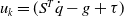
where
 ${x_1=\hat{q}, x_2=\hat{\dot{q}}, x_3=M^{-1}{\tau }_{\text{dist}} }$
in the state space.
${x_1=\hat{q}, x_2=\hat{\dot{q}}, x_3=M^{-1}{\tau }_{\text{dist}} }$
in the state space.
 ${\beta _1, \beta _2, \beta _3 }$
are diagonal matrices need to be designed.
${\beta _1, \beta _2, \beta _3 }$
are diagonal matrices need to be designed.
Then, the estimated lumped disturbances can be given by
 \begin{equation} \begin{aligned}{ \hat{{\tau }}_{\text{dist}} = M \cdot x_3 } \end{aligned} \end{equation}
Remarks: The features of ESO.orig observer are the following:
-
(1) The inversion of the inertia matrix (
${M^{-1}}$
) is needed. -
(2) There are three observer gains that need to be tuned.
-
(3) This observer works for constant payload, but not for time-varying payload.

2.8. Observer 5.2: ESO.modi
To avoid the inverse of the inertia matrix, a modified version of extended state observer (ESO.modi) [Reference Ren, Dong, Wu and Chen21] is presented below. The ESO.modi, a modified second-order linear ESO is given by
 \begin{equation} \begin{cases}{\dot{x}_1= - \beta _1 e_{1} + x_2 + ({\tau } + S^T \dot{q}-g) } \\{\dot{x}_2= - \beta _2 e_{1} } \\{e_{1} = x_1 - p } \\ \end{cases} \end{equation}
where
 ${x_1=\hat{p}, x_2=\hat{{\tau }}_{\text{ext}} }$
in the state space,
${x_1=\hat{p}, x_2=\hat{{\tau }}_{\text{ext}} }$
in the state space,
 ${p= M \dot{q}}$
is the generalized momentum of the robot,
${p= M \dot{q}}$
is the generalized momentum of the robot,
 ${\beta _1, \beta _2 }$
are diagonal gain matrices which are usually selected such that the corresponding state space matrix
${\beta _1, \beta _2 }$
are diagonal gain matrices which are usually selected such that the corresponding state space matrix
 ${A}$
is Hurwitz and has real negative eigenvalues.
${A}$
is Hurwitz and has real negative eigenvalues.
Then, the estimated lumped disturbances can be given by
 \begin{equation} \begin{aligned}{ \hat{{\tau }}_{\text{ext}} = x_2 } \end{aligned} \end{equation}
Remarks: The feature of ESO.modi are the following [Reference Ren, Dong, Wu and Chen21]:
-
(1) The phase lag is decreased by reducing the observer order compared to the ESO.orig observer.
-
(2) No need for the inversion of the inertia matrix (
${M^{-1}}$
). -
(3) There are two observer gains that need to be tuned.
-
(4) For scenarios of constant disturbance and time-varying disturbance, the observer gains need to be tuned separately in order for optimal results in each scenario. In other words, one set of observer gains is not suitable for both scenarios.
-
(5) The disturbance tracking error of ESO converges asymptotically when the dynamic model is available, while it is bounded when the dynamic model is not available [Reference Ren, Dong, Wu and Chen21, Reference Zheng, Gao and Gao32].

2.9. Observer 5.3: ESO.impr
The improved version of extended state observer (ESO.impr) [Reference Sebastian, Li, Crocher, Kremers, Tan and Oetomo12] that is extended especially for time-varying external disturbances is presented below. The ESO.impr, an improved third-order linear ESO, can be given by
 \begin{equation} \begin{cases}{\dot{x}_1= \frac{\beta _1}{\epsilon } e_{1} + x_2 } \\{\dot{x}_2= \frac{\beta _2}{\epsilon ^2} e_{1} + M^{-1} (x_3 +{\tau }) - M^{-1} ( S \dot{q} + g ) } \\{\dot{x}_3= \frac{1}{\epsilon ^3} e_{1} } \\{e_{1} = q - x_1 } \\ \end{cases} \end{equation}
where
 ${x_1=\hat{q}, x_2=\hat{\dot{q}}, x_3=\hat{{\tau }}_{ext} }$
in the state space,
${x_1=\hat{q}, x_2=\hat{\dot{q}}, x_3=\hat{{\tau }}_{ext} }$
in the state space,
 ${ (\beta _1, \beta _2, \epsilon ) }$
are positive scalar parameters need to be designed. For the full designing procedures and theoretical analysis of this ESO.impr, please refer to ref. [Reference Sebastian, Li, Crocher, Kremers, Tan and Oetomo12].
${ (\beta _1, \beta _2, \epsilon ) }$
are positive scalar parameters need to be designed. For the full designing procedures and theoretical analysis of this ESO.impr, please refer to ref. [Reference Sebastian, Li, Crocher, Kremers, Tan and Oetomo12].
Then, the estimated lumped disturbances can be given by
 \begin{equation} \begin{aligned}{ \hat{{\tau }}_{\text{ext}} = x_3 } \end{aligned} \end{equation}
Remarks: The features of ESO.impr are the following [Reference Sebastian, Li, Crocher, Kremers, Tan and Oetomo12]:
-
(1) The inversion of the inertia matrix (
${M^{-1}}$
) is needed. -
(2) There are three scalar observer gains that need to be tuned which make the tuning relatively simpler than ESO.orig and ESO.modi.
-
(3) The ESO.impr is a linear ESO but it works for nonlinear dynamic systems and a large class of external forces.

3. Simulations and results
3.1. Robotic system
A 3-DOF PHANToM Premium 1.5A robot (3D Systems, Inc., Cary, NC, USA) is used for simulations in this paper in order to test the disturbance tracking performance of different observers. To build a virtual model of this robot, the kinematic model and dynamic model of the PHANToM robot are reconstructed based on ref. [Reference Çavuşoğlu, Feygin and Tendick33]. All the simulations are conducted by using MATLAB/Simulink (version R2020a, MathWorks Inc., Natick, MA, USA), which is running on a computer with a 3.70 GHz Intel(R) Core(TM) i5-9600K CPU and a Windows 10 Education 64-bit operating system. The control rate of the virtual robot is set as 1000 Hz, while the sampling rate for acquiring data is 500 Hz.
3.2. Robot kinematics
A thorough exploration of the kinematics and dynamics of the 3-DOF Phantom Premium 1.5A can refer [Reference Çavuşoğlu, Feygin and Tendick33]. Additionally, a Denavit-Hartenberg (DH) table for this robot is provided in Table I. The corresponding frames’ definitions are illustrated in Fig. 1. Please note that the base frame of this robot is defined to be coincident with the initial robot end-effector (EE) position (see the gray pose in Fig. 1).
Table I. Denavit-Hartenberg (DH) parameters for the 3-DOF Phantom Premium 1.5A robot’s kinematic chain (for the homogeneous transform in the modified convention).
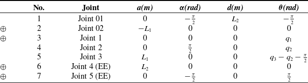
Note:
•
 $L_1$
and
$L_1$
and
 $L_2$
are link length.
$L_2$
are link length.
• Symbol
 $\oplus$
means that the DH parameters of these two adjacent joints can be directly summed together, respectively, to be as one joint.
$\oplus$
means that the DH parameters of these two adjacent joints can be directly summed together, respectively, to be as one joint.
• Joint
 $01$
,
$01$
,
 $02$
, and
$02$
, and
 $5$
are virtual joints that are only used for transforming one frame to another desired one via translation and/or rotation.
$5$
are virtual joints that are only used for transforming one frame to another desired one via translation and/or rotation.
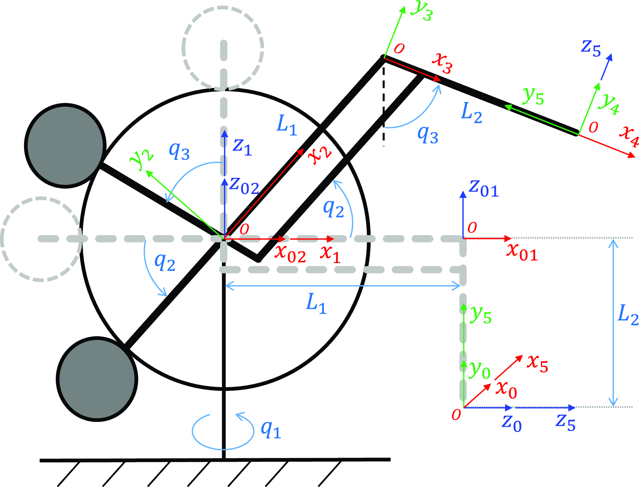
Figure 1. Schematic of the 3-DOF Phantom Premium 1.5A robot and frame attachment to each joint. Frame {0} is the base frame while frame {5} is the end-effector (EE) frame.
 $L_1, L_2$
are link lengths.
$L_1, L_2$
are link lengths.
 $q_1, q_2, q_3$
are joint angle variables.
$q_1, q_2, q_3$
are joint angle variables.
According to the DH parameters in Table I and the frames determined in Fig. 1, the homogeneous transformation matrix
 ${T}$
from EE frame {5} to base frame {0} can be obtained as
${T}$
from EE frame {5} to base frame {0} can be obtained as
 \begin{equation} \begin{aligned}{T} &= \left [\begin{array}{r@{\quad}r@{\quad}r@{\quad}r} c_1,& -s_1 s_3,& c_3 s_1,& s_1 (L_1 c_2 + L_2 s_3) \\ 0,& c_3,& s_3,& L_2 - L_2 c_3 + L_1 s_2 \\ -s_1,& -c_1 s_3,& c_1 c_3,& L_1 c_1 c_2 - L_1 + L_2 c_1 s_3 \\ 0,& 0,& 0,& 1 \\ \end{array}\right ] \end{aligned} \end{equation}
where
 $s_i, c_i$
represent
$s_i, c_i$
represent
 $\sin (q_i), \cos (q_i), i=1,2,3$
, respectively.
$\sin (q_i), \cos (q_i), i=1,2,3$
, respectively.
 $L_1, L_2$
are link lengths.
$L_1, L_2$
are link lengths.
The Jacobian matrix
 ${J}$
can be expressed by
${J}$
can be expressed by
 \begin{equation} \begin{aligned}{J} &= \left [\begin{array}{r@{\quad}r@{\quad}r} c_1 (L_1 c_2 + L_2 s_3),& -L_1 s_1 s_2,& L_2 c_3 s_1 \\ 0,& L_1 c_2,& L_2 s_3 \\ -s_1 (L_1 c_2 + L_2 s_3),& -L_1 c_1 s_2,& L_2 c_1 c_3 \\ 0,& 0,& -c_1 \\ 1,& 0,& 0 \\ 0,& 0,& s_1 \\ \end{array}\right ] \end{aligned} \end{equation}
Note that the Jacobian matrix here is the space Jacobian which can be calculated from the body Jacobian used in ref. [Reference Çavuşoğlu, Feygin and Tendick33]. In this paper, we only use the upper 3-by-3 linear part of the Jacobian in Eq. (46), which means that the rotational angles in Cartesian space are ignored.
3.3. Parameterization
For all simulations in the remaining part of this paper, the values assigned to the parameters are summarized in Table II.
Table II. Parameterization for simulations and experiments.
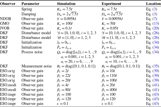
Note:
 ${I} \in \mathbb{R}^{3 \times 3}$
denote identity matrix.
${I} \in \mathbb{R}^{3 \times 3}$
denote identity matrix.
It has been proved in our earlier work that by integrating an impedance controller and an observer, an accurate impedance control can be achieved in a trajectory tracking task when the actual velocity and acceleration converge to the desired ones [Reference Li, Badre, Taghirad and Tavakoli23]. It is noteworthy that the observer estimation accuracy is not affected by the trajectory tracking accuracy. In other words, even if the trajectory tracking performance is poor (e.g., due to a small stiffness gain setting in the impedance model, or uncompensated disturbances), the observer will still have an accurate estimation of the lumped uncertainties.
In order to explore the disturbance tracking performance of different observers integrated with an impedance controller, a figure-eight trajectory expressed by Eq. (47) is employed in the simulated trajectory tracking task.
 \begin{equation} \begin{cases} x_{d} = R \sin (\frac{2\pi }{t_1} t) \cos (\frac{2\pi }{t_1} t) \\ y_{d} = R \sin (\frac{2\pi }{t_1} t) + R \\ z_{d} = 0 \\ \end{cases} \end{equation}
where
 $R=0.02$
m is the amplitude of the figure-eight trajectory,
$R=0.02$
m is the amplitude of the figure-eight trajectory,
 $t_1 = 5$
s is the period for generating a full cycle.
$t_1 = 5$
s is the period for generating a full cycle.
Then, two typical types of external disturbance, that is, constant payload and time-varying payload, are applied to the robot EE separately. The constant payload is
 $22$
g, and the time-varying payload is represented by a set of sinusoidal curves given by Eq. (48).
$22$
g, and the time-varying payload is represented by a set of sinusoidal curves given by Eq. (48).
 \begin{equation} \begin{cases} Fx_{d} = a_1 \sin (\frac{2\pi }{t_1} t) \\ Fy_{d} = a_2 \sin (\frac{2\pi }{t_2} t) \\ Fz_{d} = a_3 \sin (\frac{2\pi }{t_3} t) \\ \end{cases} \end{equation}
where
 $t_1=2$
,
$t_1=2$
,
 $t_2=5$
,
$t_2=5$
,
 $t_3=2$
are cycles of the desired time-varying EE payload for each axis in units of second,
$t_3=2$
are cycles of the desired time-varying EE payload for each axis in units of second,
 $a_1=0.01$
,
$a_1=0.01$
,
 $a_2=0.2$
,
$a_2=0.2$
,
 $a_3=0.01$
are the corresponding amplitudes in units of Newton.
$a_3=0.01$
are the corresponding amplitudes in units of Newton.
3.4. Individual observer simulations
In this section, the trajectory tracking performance of each observer under three types of disturbances is presented, that is, ideal dynamic model without any disturbances, dynamic model under a constant disturbance, and dynamic model under a sinusoidal disturbance. For the scenario of no disturbances, no observers need to be implemented, and the trajectory tracking task performance under an impedance controller is taken as a reference. For the scenarios of constant disturbance and sinusoidal disturbances, each of the introduced observers, that is, NDOB, GMO, JVOB, DKF, ESO.orig, ESO.modi, and ESO.impr, will be implemented to track the disturbance and thus do a compensation in the control law. The disturbance tracking performance of each observer will be presented, respectively in the following part. Note that the observer gains in the simulations are tuned by using a trial and error method based on a binary searching strategy.
With an ideal dynamic model, the figure-eight trajectory tracking performance under an impedance controller (3) is shown in Fig. 2a, b. The figure shows that the impedance controller with properly tuned impedance gains (
 ${M_m, D_m, K_m}$
) can accurately track the desired figure-eight trajectory when none of any disturbances or uncertainties are involved. However, when a constant payload of
${M_m, D_m, K_m}$
) can accurately track the desired figure-eight trajectory when none of any disturbances or uncertainties are involved. However, when a constant payload of
 $22$
g is added to the robot EE, the trajectory tracking performance is affected as shown in Fig. 2c. And when a time-varying sinusoidal payload (48) is added to the robot EE, the affected tracking performance is shown in Fig. 2d. From Fig. 2c, d we can see that, if disturbance exists in the control system but not be compensated, the trajectory tracking performance can be significantly affected.
$22$
g is added to the robot EE, the trajectory tracking performance is affected as shown in Fig. 2c. And when a time-varying sinusoidal payload (48) is added to the robot EE, the affected tracking performance is shown in Fig. 2d. From Fig. 2c, d we can see that, if disturbance exists in the control system but not be compensated, the trajectory tracking performance can be significantly affected.
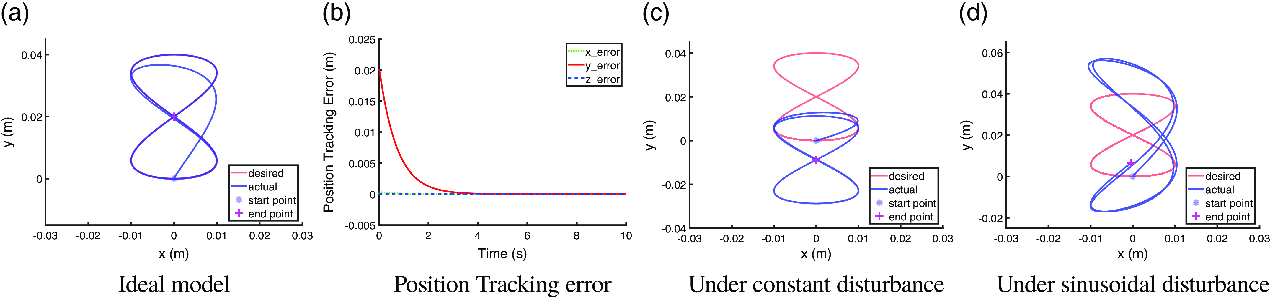
Figure 2. Simulation of figure-eight trajectory tracking under different types of disturbance. (a) Ideal dynamic model without any disturbances; (b) position tracking error with the ideal dynamic model; (c) trajectory tracking performance under a constant disturbance of a
 $22$
g payload; (d) trajectory tracking performance under a sinusoidal disturbance.
$22$
g payload; (d) trajectory tracking performance under a sinusoidal disturbance.
With implementing the observer of NDOB, the trajectory tracking performance in the constant-payload scenario and time-varying-payload scenario are shown in Fig. 3a, b and Fig. 4a, b, respectively, while the disturbance tracking performance in two scenarios is shown in Fig. 3c, d and Fig. 4c, d, respectively. Figures 3 and 4 show that with NDOB observer, both the constant and sinusoidal disturbance can be accurately estimated and compensated, thus an accurate trajectory tracking performance can be recovered compared to the reference in Fig. 2. Note that the disturbance tracking can reach a steady state within
 $0.1$
s in both scenarios. For the term steady state, we define it as when the actual values are within 5% of the target value (for constant disturbances) or when the disturbance tracking error falls into its upper/lower bound for the first time (for time-varying disturbances).
$0.1$
s in both scenarios. For the term steady state, we define it as when the actual values are within 5% of the target value (for constant disturbances) or when the disturbance tracking error falls into its upper/lower bound for the first time (for time-varying disturbances).
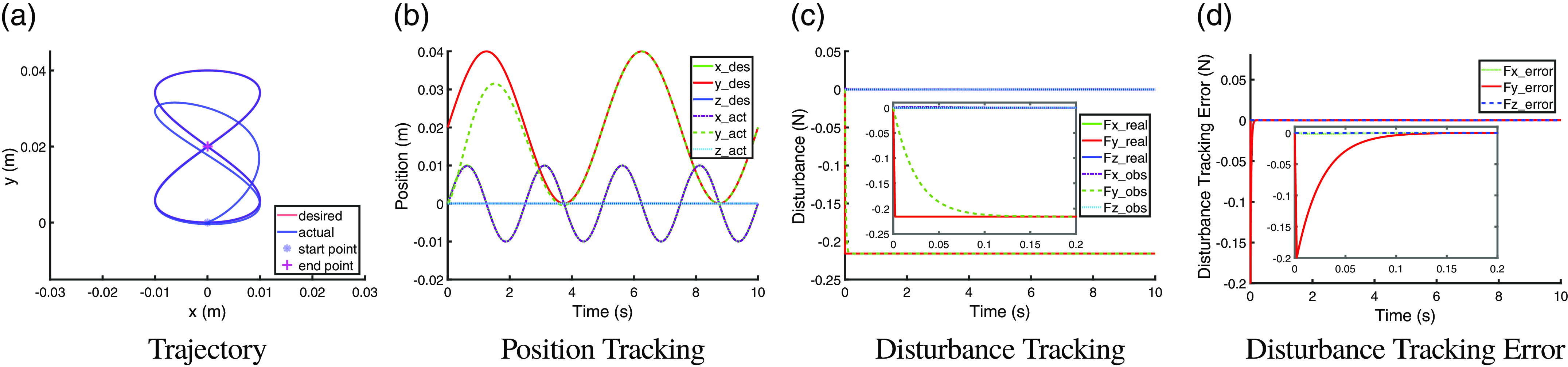
Figure 3. Trajectory tracking performance and disturbance tracking performance with NDOB observer under a constant disturbance of a constant
 $22$
g payload.
$22$
g payload.
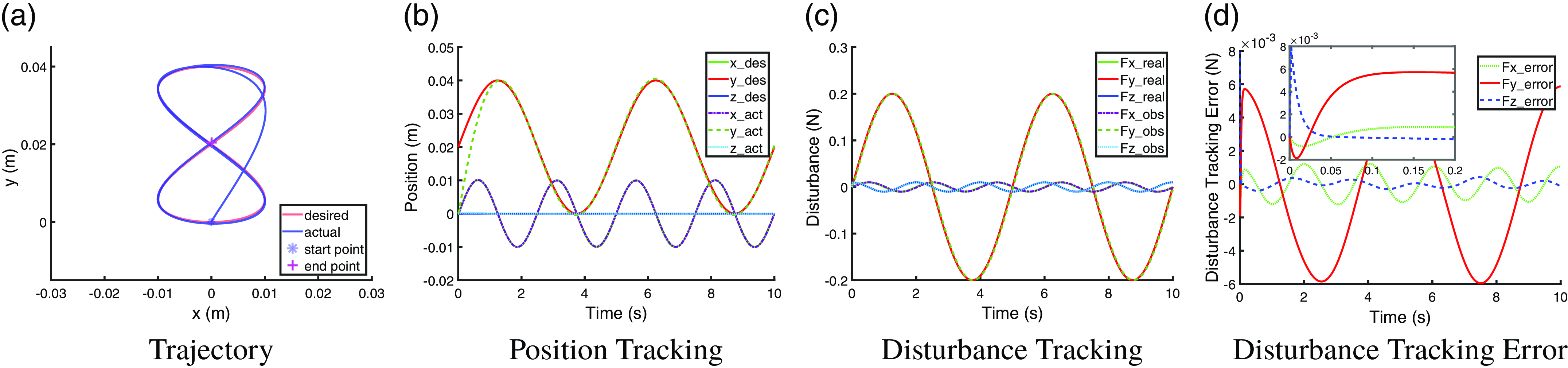
Figure 4. Trajectory tracking performance and disturbance tracking performance with NDOB observer under a time-varying disturbance of a sinusoidal payload.
With implementing the observer of GMO, the trajectory tracking performance in constant-payload scenario and time-varying-payload scenario are shown in Fig. 5a, b and Fig. 6a, b, respectively. The disturbance tracking performance in two scenarios is shown in Fig. 5c, d and Fig. 6c, d, respectively. Figures 5 and 6 show that with GMO observer, both the constant and sinusoidal disturbance can be accurately estimated and compensated, thus an accurate trajectory tracking performance can be recovered compared to the reference in Fig. 2. The disturbance tracking can reach a steady state within
 $0.1$
s in both scenarios. The disturbance tracking performance of GMO is very similar to that of NDOB.
$0.1$
s in both scenarios. The disturbance tracking performance of GMO is very similar to that of NDOB.
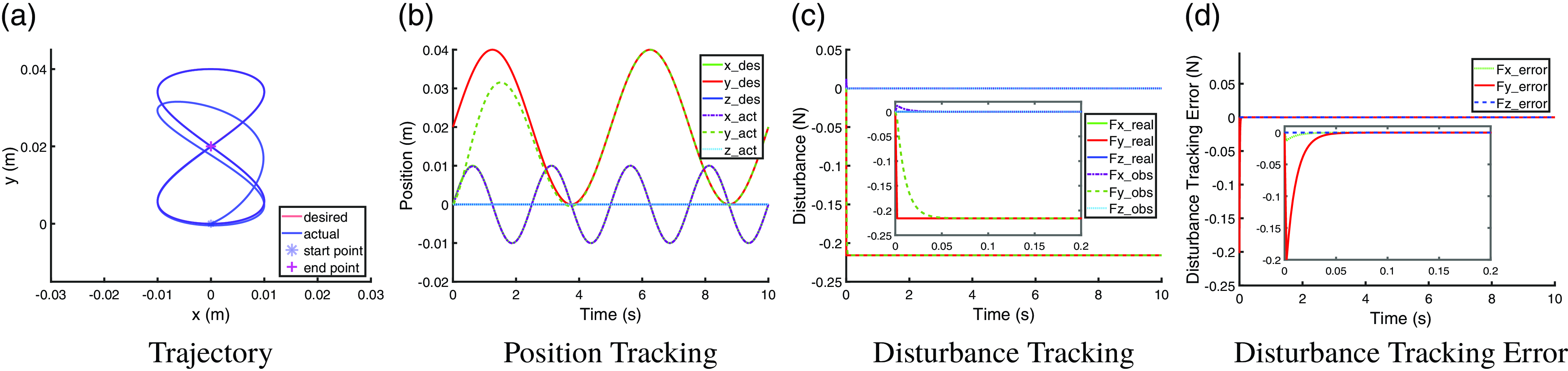
Figure 5. Trajectory tracking performance and disturbance tracking performance with GMO observer under a constant disturbance of a constant
 $22$
g payload.
$22$
g payload.
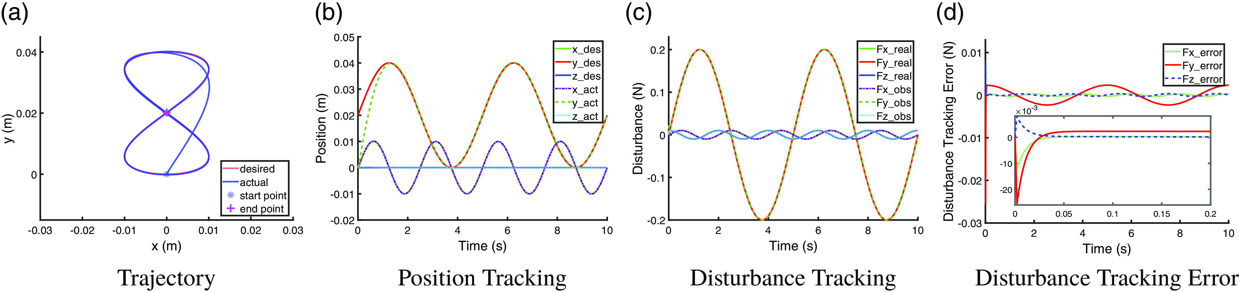
Figure 6. Trajectory tracking performance and disturbance tracking performance with GMO observer under a time-varying disturbance of a sinusoidal payload.
With implementing the observer of JVOB, the trajectory tracking performance in constant-payload scenario and time-varying-payload scenario are shown in Fig. 7a, b and Fig. 8a, b, respectively. The disturbance tracking performance in two scenarios are shown in Fig. 7c, d and Fig. 8c, d, respectively. Figures 7 and 8 show that, by implementing JVOB observer to compensate for disturbances, an accurate trajectory tracking performance is able to be recovered in both the constant disturbance scenario and the time-varying-disturbance scenario when comparing to the reference in Fig. 2. The disturbance tracking can reach a steady state within
 $0.1$
s in both scenarios. Also, we can find that the disturbance tracking performance of JVOB is very similar to that of NDOB and GMO.
$0.1$
s in both scenarios. Also, we can find that the disturbance tracking performance of JVOB is very similar to that of NDOB and GMO.
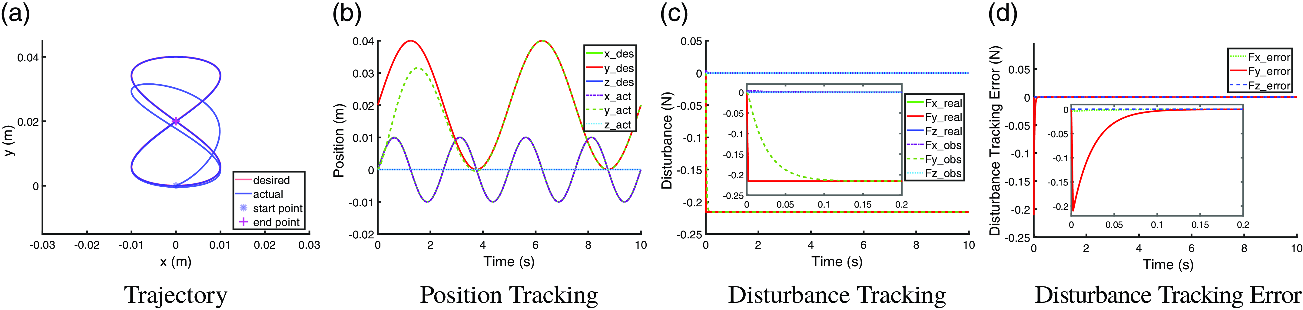
Figure 7. Trajectory tracking performance and disturbance tracking performance with JVOB observer under a constant disturbance of a constant
 $22$
g payload.
$22$
g payload.
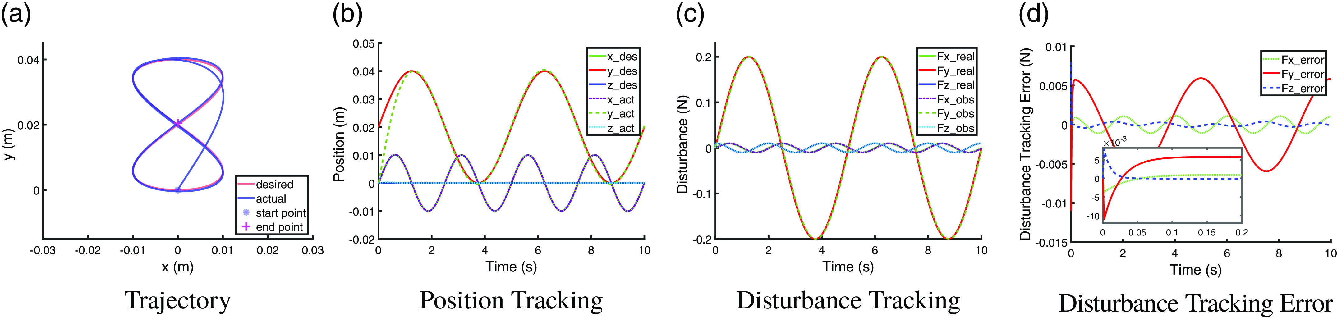
Figure 8. Trajectory tracking performance and disturbance tracking performance with JVOB observer under a time-varying disturbance of a sinusoidal payload.
With implementing the observer of DKF, the trajectory tracking performance in constant-payload scenario and time-varying-payload scenario are shown in Fig. 9a, b and Fig. 10a, b, respectively. The disturbance tracking performance in two scenarios is shown in Fig. 9c, d and Fig. 10c, d, respectively. Figures 9 and 10 show that with DKF observer, both the constant and time-varying disturbance can be accurately estimated and compensated; thus, an accurate trajectory tracking performance can be recovered to be normal compared to the reference in Fig. 2. The disturbance tracking can reach a steady state within
 $0.1$
s in both scenarios. It is interesting to find that the disturbance tracking performance of DKF in this specific case is very similar to that of NDOB, GMO, and JVOB.
$0.1$
s in both scenarios. It is interesting to find that the disturbance tracking performance of DKF in this specific case is very similar to that of NDOB, GMO, and JVOB.

Figure 9. Trajectory tracking performance and disturbance tracking performance with DKF observer under a constant disturbance of a constant
 $22$
g payload.
$22$
g payload.

Figure 10. Trajectory tracking performance and disturbance tracking performance with DKF observer under a time-varying disturbance of a sinusoidal payload.
With implementing the observer of ESO.orig, the trajectory tracking performance in constant-payload scenario and time-varying-payload scenario are shown in Fig. 11a, b and Fig. 12a, b, respectively. The disturbance tracking performance in two scenarios is shown in Fig. 11c, d and Fig. 12c, d, respectively. Comparing the disturbance tracking performance of ESO.orig in Figs. 11 and 12, we can see that ESO.orig observer can track constant disturbance but not time-varying sinusoidal disturbance. Also, for tracking constant disturbance, it takes a significantly long time (about
 $6$
s) to reach a steady state. Since the ESO.orig observer cannot track time-varying disturbance, the figure-eight trajectory tracking is still distorted as shown in Fig. 12a when comparing it with the corresponding reference in Fig. 2d.
$6$
s) to reach a steady state. Since the ESO.orig observer cannot track time-varying disturbance, the figure-eight trajectory tracking is still distorted as shown in Fig. 12a when comparing it with the corresponding reference in Fig. 2d.

Figure 11. Trajectory tracking performance and disturbance tracking performance with ESO.orig observer under a constant disturbance of a constant
 $22$
g payload.
$22$
g payload.

Figure 12. Trajectory tracking performance and disturbance tracking performance with ESO.orig observer under a time-varying disturbance of a sinusoidal payload.
With implementing the observer of ESO.modi, the trajectory tracking performance in constant-payload scenario and time-varying-payload scenario are shown in Fig. 13a, b and Fig. 14a, b, respectively. The disturbance tracking performance in two scenarios is shown in Fig. 13c, d and Fig. 14c, d, respectively. For tracking constant disturbance in Fig. 13, the disturbance can be accurately estimated and compensated; thus, trajectory tracking performance is recovered to be normal. For tracking time-varying disturbance in Fig. 14, although the disturbance tracking error is relatively large compared to the results from NDOB, GMO, JVOB, and DKF, the trajectory tracking performance is recovered to a large extent when comparing to the reference in Fig. 2. Note that it also takes a relatively long time for the disturbance tracking to reach a steady state (about
 $2$
s) in both scenarios.
$2$
s) in both scenarios.

Figure 13. Trajectory tracking performance and disturbance tracking performance with ESO.modi observer under a constant disturbance of a constant
 $22$
g payload.
$22$
g payload.

Figure 14. Trajectory tracking performance and disturbance tracking performance with ESO.modi observer under a time-varying disturbance of a sinusoidal payload.
With implementing the observer of ESO.impr, the trajectory tracking performance in constant-payload scenario and time-varying-payload scenario are shown in Fig. 15a, b and Fig. 16a, b, respectively. The disturbance tracking performance in two scenarios is shown in Fig. 15c, d and Fig. 16c, d, respectively. For tracking constant disturbance in Fig. 15, the disturbance can be accurately estimated and compensated; thus, trajectory tracking performance is recovered to be normal. For tracking time-varying disturbance in Fig. 16, ESO.impr is better than ESO.orig and ESO.modi in terms of disturbance tracking error, but not as good as NDOB, GMO, JVOB, and DKF in the same simulated scenario. It takes a relatively long time for the disturbance tracking to reach a steady state (about
 $1$
s) in both disturbance scenarios.
$1$
s) in both disturbance scenarios.

Figure 15. Trajectory tracking performance and disturbance tracking performance with ESO.impr observer under a constant disturbance of a constant
 $22$
g payload.
$22$
g payload.

Figure 16. Trajectory tracking performance and disturbance tracking performance with ESO.impr observer under a time-varying disturbance of a sinusoidal payload.
3.5. Comparing observers under constant disturbance
Here in this section, we put the disturbance tracking errors of all observers in the same figure for an intuitive and qualitative comparison. Note that these comparisons are expected to provide an intuitive sense of the possible behaviors of different observers in the same simulated scenario rather than quantitative analyses. It should be noted that the behavior of an observer may be varying due to many factors, such as gain tuning or a specific application scenario setting. One observer may have better performance than others in one specific scenario, but may also have worse performance in another scenario.
Figure 17 shows the disturbance tracking error in Cartesian space when different observers are implemented to track a constant payload of
 $22$
g (
$22$
g (
 $-0.2158$
N along the
$-0.2158$
N along the
 $y$
-axis). Since the ESO.orig observer has poor disturbance tracking performance especially on time-varying disturbance, it does not appear in the figure. As clearly can be seen in the figure, the ESO.modi and ESO.impr observer have remarkably poor disturbance tracking performance compared to other observers.
$y$
-axis). Since the ESO.orig observer has poor disturbance tracking performance especially on time-varying disturbance, it does not appear in the figure. As clearly can be seen in the figure, the ESO.modi and ESO.impr observer have remarkably poor disturbance tracking performance compared to other observers.
Table III. MSE of constant disturbance tracking in steady state (
 $[5,10]$
s).
$[5,10]$
s).
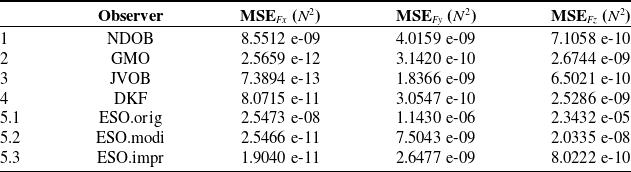
Note: The tracked external disturbance is a constant payload of
 $22$
g (
$22$
g (
 $-0.2158$
N along the
$-0.2158$
N along the
 $y$
-axis).
$y$
-axis).

Figure 17. Disturbance tracking errors of different observers in the same constant-payload scenario.
The mean squared error (MSE) of constant disturbance tracking in steady state (
 $[5,10]$
s) is summarized in Table III, and the corresponding bar chart is shown in Fig. 18 (note that ESO.orig is excluded due to its significantly higher MSE than other observers). Generally, all observers have relatively good disturbance tracking performance considering that the MSE is at the order of magnitude of
$[5,10]$
s) is summarized in Table III, and the corresponding bar chart is shown in Fig. 18 (note that ESO.orig is excluded due to its significantly higher MSE than other observers). Generally, all observers have relatively good disturbance tracking performance considering that the MSE is at the order of magnitude of
 $10^{-8}$
. This is reasonable since the disturbance is a simple constant payload.
$10^{-8}$
. This is reasonable since the disturbance is a simple constant payload.

Figure 18. MSE of different observers in the same constant-payload scenario in steady state (
 $[5,10]$
s).
$[5,10]$
s).
In summary, for the disturbance-tracking performance in a simple constant-payload scenario, all observers can reach a relatively high tracking accuracy in the steady state except the ESO.orig. However, the observers of NDOB, GMO, JVOB, and DKF have significantly faster convergence speeds than the observers of ESO.modi and ESO.impr.
3.6. Comparing observers under sinusoidal disturbance
Figure 19 shows the disturbance tracking errors when different observers are implemented to track a time-varying sinusoidal payload with amplitude
 $[0.01,0.2,0.01]$
N. As mentioned earlier, the ESO.orig observer only works for constant disturbances but not time-varying disturbances, so it does not appear in the figure. As clearly can be seen in the figure, the ESO.modi observer has the worst disturbance tracking performance among all observers presented in the figure.
$[0.01,0.2,0.01]$
N. As mentioned earlier, the ESO.orig observer only works for constant disturbances but not time-varying disturbances, so it does not appear in the figure. As clearly can be seen in the figure, the ESO.modi observer has the worst disturbance tracking performance among all observers presented in the figure.

Figure 19. Disturbance tracking errors of different observers in the same time-varying sinusoidal payload scenario.
The MSE of sinusoidal disturbance tracking in steady state (
 $[5,10]$
s) is summarized in Table IV, and the corresponding bar chart is shown in Fig. 20 (note that ESO.orig is excluded in the bar chart due to its significantly higher MSE than other observers). As can be seen in the figure, the ESO.modi observer has the worst disturbance-tracking performance among all observers presented in the figure. Note that the sinusoidal time-varying payload is with amplitude
$[5,10]$
s) is summarized in Table IV, and the corresponding bar chart is shown in Fig. 20 (note that ESO.orig is excluded in the bar chart due to its significantly higher MSE than other observers). As can be seen in the figure, the ESO.modi observer has the worst disturbance-tracking performance among all observers presented in the figure. Note that the sinusoidal time-varying payload is with amplitude
 $[0.01,0.2,0.01]$
N, which means that the disturbance along
$[0.01,0.2,0.01]$
N, which means that the disturbance along
 $y$
-axis has the highest amplitude (
$y$
-axis has the highest amplitude (
 $0.2$
N).
$0.2$
N).
Table IV. MSE of sinusoidal disturbance tracking in steady state (
 $[5,10]$
s).
$[5,10]$
s).
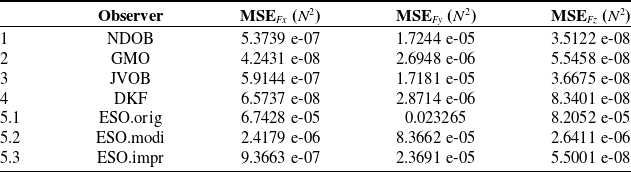
Note: The tracked external disturbance is a sinusoidal time-varying payload with amplitude (
 $[0.01,0.2,0.01]$
N).
$[0.01,0.2,0.01]$
N).

Figure 20. MSE of different observers in the same sinusoidal payload scenario in steady state (
 $[5,10]$
s).
$[5,10]$
s).
In summary, for the disturbance-tracking performance in a sinusoidal payload scenario, all observers are capable of tracking the sinusoidal disturbance except ESO.orig. However, unlike their performance in the constant-payload scenario, their tracking accuracy cannot converge to zero errors in the steady state anymore. Instead, their disturbance-tracking errors in the steady state are bounded. In this specific case, the observers of GMO and DKF have the highest disturbance-tracking accuracy, and the observers of NDOB, JVOB, and ESO.impr have relatively lower tracking accuracy, while the observer of ESO.modi has the lowest tracking accuracy. Similar to the constant-payload scenario, the observers of NDOB, GMO, JVOB, and DKF still have significantly faster convergence speeds than the observers of ESO.modi and ESO.impr.
3.7. Comparing observers under harmonic disturbance with Gaussian noise
In this section, a more realistic scenario is simulated where the external disturbance is a set of Fourier series functions (i.e., harmonics) given by
 \begin{equation} \small \begin{cases} F_x = a_1 \sin ( \frac{2 \pi n_1}{t_1} t) + a_2 \sin ( \frac{2 \pi n_2}{t_1} t-\phi _2) + a_3 \sin ( \frac{2 \pi n_3}{t_1} t-\phi _3) \\[3pt] F_y = a_1 \cos ( \frac{2 \pi n_1}{t_1} t) + a_2 \cos ( \frac{2 \pi n_2}{t_1} t-\phi _2) + a_3 \cos ( \frac{2 \pi n_3}{t_1} t-\phi _3) \\[3pt] F_z = a_1 \cos ( \frac{2 \pi n_1}{t_1} t) + a_2 \sin ( \frac{2 \pi n_2}{t_1} t-\phi _2) + a_3 \cos ( \frac{2 \pi n_3}{t_1} t-\phi _3) \\ \end{cases} \end{equation}
where
 $F_x, F_y, F_z$
are the force components of the time-varying payload expressed in Cartesian space, and
$F_x, F_y, F_z$
are the force components of the time-varying payload expressed in Cartesian space, and
 $t_1=10$
,
$t_1=10$
,
 $a_1=0.1$
,
$a_1=0.1$
,
 $a_2=0.15$
,
$a_2=0.15$
,
 $a_3=0.05$
,
$a_3=0.05$
,
 $n_1=1$
,
$n_1=1$
,
 $n_2=2$
,
$n_2=2$
,
 $n_3=3$
,
$n_3=3$
,
 $\phi _2=\frac{1}{2} \pi$
,
$\phi _2=\frac{1}{2} \pi$
,
 $\phi _3= \pi$
. Based on Eq. (49), a pseudo-randomly generated zero-mean Gaussian noise is added to each axis of the time-varying payload while the seeds for the random number generator remain the same over the simulations of different observers.
$\phi _3= \pi$
. Based on Eq. (49), a pseudo-randomly generated zero-mean Gaussian noise is added to each axis of the time-varying payload while the seeds for the random number generator remain the same over the simulations of different observers.
Figure 21 shows the disturbance tracking performance of each observer when a complex harmonic disturbance with Gaussian noise is employed. Again, as mentioned earlier, the ESO.orig observer does not work for time-varying disturbances, so it does not appear in the figure. As can be seen in the figure, all observers have relatively good disturbance tracking performance in the steady state, except that different behaviors may exist for different observers in the initial transition period.

Figure 21. Disturbance tracking performance of different observers when the time-varying payload is complex harmonics with Gaussian noise.
The MSE of noisy harmonic disturbance tracking in steady state (
 $[5,10]$
s) is summarized in Table V, and the corresponding bar chart is shown in Fig. 22 (note that ESO.orig is excluded in the bar chart due to its significantly higher MSE than other observers). As can be seen in the figure, the ESO.modi observer has the worst disturbance-tracking performance among all observers presented in terms of MSE. Note that the harmonic disturbance with Gaussian noise is with amplitude
$[5,10]$
s) is summarized in Table V, and the corresponding bar chart is shown in Fig. 22 (note that ESO.orig is excluded in the bar chart due to its significantly higher MSE than other observers). As can be seen in the figure, the ESO.modi observer has the worst disturbance-tracking performance among all observers presented in terms of MSE. Note that the harmonic disturbance with Gaussian noise is with amplitude
 $[0.3,0.3,0.3]$
N, which means that the disturbance along each axis has the same amplitude (
$[0.3,0.3,0.3]$
N, which means that the disturbance along each axis has the same amplitude (
 $0.3$
N).
$0.3$
N).
Table V. MSE of harmonic disturbance with Gaussian noise tracking in steady state (
 $[5,10]$
s).
$[5,10]$
s).
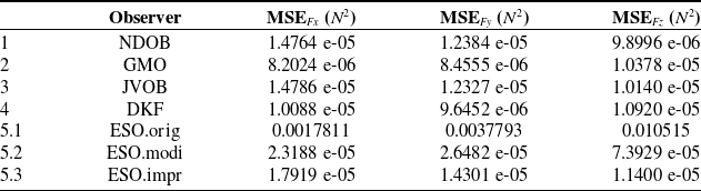
Note: The tracked external disturbance is a Fourier series time-varying payload with amplitude (
 $[0.3,0.3,0.3]$
N).
$[0.3,0.3,0.3]$
N).

Figure 22. MSE of different observers in steady state (
 $[5,10]$
s) when the time-varying disturbance is complex harmonic with Gaussian noise.
$[5,10]$
s) when the time-varying disturbance is complex harmonic with Gaussian noise.
In summary, for the disturbance-tracking performance in a complex harmonic disturbance scenario, all observers can track the harmonic disturbance except ESO.orig. Similar to the constant-payload scenario and the sinusoidal payload scenario, the observers of NDOB, GMO, JVOB, and DKF have significantly faster convergence speeds than the observers of ESO.modi and ESO.impr.
4. Experiments and results
Although the simulations are the main focus of this work, physical experiments are also conducted to demonstrate the effect of different observers on dealing with real-scenario disturbances. The same robotic system used in simulations, that is, the 3-DOF PHANToM Premium 1.5A robot, is also used for physical experiments. Quarc real-time control software (Quanser Inc., Markham, ON, Canada) is used for real-time control on the 3-DOF physical robot while the control rate is 1000 Hz. Same as the simulations, the impedance controller (3) and the figure-eight trajectory (47) are employed in the experimental trajectory tracking task. The parameterization for experiments is summarized in Table II. A demonstration video of the experiments with implementing different observers is attached.Footnote 1
For tuning the observer gains in the experiments, all of them are started with the same gains used in the simulations. For NDOB, GMO, JVOB, and DKF, using the exact simulation gains in experiments will cause robot chattering, thus the observer gains are tuned down correspondingly by trial and error method. For ESO.orig and ESO.modi, the gains are tuned up correspondingly in order for better trajectory tracking performance, while ESO.impr uses the exact same gains as that used in the simulations.
For the disturbances in the experiments, dynamic model errors and unmodeled frictions always exist. There are two scenarios taken as references, that is, Ref.1, and Ref.2, as shown in Fig. 23a and Fig. 23b respectively. Both Ref.1, and Ref.2 are implemented with impedance controller but without any observer, and the only difference is that Ref.1 involves model errors and unmodeled frictions, while Ref.2 involves model errors, unmodeled frictions, and an external constant payload (
 $22$
g). As can be seen in Fig. 23a, the actual trajectory is shrunken compared to the desired one due to the model errors and unmodeled frictions, while in Fig. 23b, the actual trajectory is not only shrunken but also shifted downward due to the additional external payload.
$22$
g). As can be seen in Fig. 23a, the actual trajectory is shrunken compared to the desired one due to the model errors and unmodeled frictions, while in Fig. 23b, the actual trajectory is not only shrunken but also shifted downward due to the additional external payload.

Figure 23. Physical experiments and results when implementing different observers.
Figure 23c–i show the trajectory tracking performance when different observers are implemented while the disturbance sources are the same as Ref.2 (Fig. 23b), that is, dynamic model errors, unmodeled frictions, and an external constant payload (
 $22$
g). As shown in Fig. 23c–i, all observers can effectively estimate and compensate for the disturbances except ESO.orig. Note that ESO.orig results in a shrunken but not downward-shifted actual trajectory (Fig. 23g) that is similar to the result in Ref.1 (Fig. 23a). This indicates that ESO.orig is not capable of dealing with dynamic model errors and unmodeled frictions which can be considered as time-varying disturbances. This is consistent with the results in simulations, that is, ESO.orig is capable of tracking constant disturbances but not time-varying disturbances.
$22$
g). As shown in Fig. 23c–i, all observers can effectively estimate and compensate for the disturbances except ESO.orig. Note that ESO.orig results in a shrunken but not downward-shifted actual trajectory (Fig. 23g) that is similar to the result in Ref.1 (Fig. 23a). This indicates that ESO.orig is not capable of dealing with dynamic model errors and unmodeled frictions which can be considered as time-varying disturbances. This is consistent with the results in simulations, that is, ESO.orig is capable of tracking constant disturbances but not time-varying disturbances.
In summary, for a physical robot system, only implementing a controller may not be able to achieve good trajectory tracking performance due to the inevitable dynamic model errors and unmodeled/inaccurate joint frictions. The dynamic model errors and unmodeled/inaccurate joint frictions may result in a shrunken trajectory, while an external constant payload attached to the robot EE may cause the actual trajectory to shift downward. When a suitable disturbance observer is implemented together with the controller, a satisfying trajectory tracking performance can be achieved due to the fact that the lumped uncertainties can be effectively estimated and compensated by the observer.
5. Discussions and conclusions
In this paper, we reviewed five typical types of disturbance observers, including GMO, JVOB, NDOB, DKF, ESO (ESO.orig, ESO.modi, ESO.impr). We presented the simulation results on disturbance tracking performances of each observer in three scenarios based on the types of disturbance, that is, a constant payload, a time-varying sinusoidal payload, and harmonic disturbance with Gaussian noise.
For the DKF method implemented in the simulations, the disturbance model is constructed as a polynomial disturbance (27) for both the sinusoidal disturbance scenario and the harmonic disturbance scenario. This is acceptable when the frequency of the disturbance is relatively low, for example, in this paper, the sinusoidal disturbance is
 $[0.5, 0.2, 0.5]$
Hz, and the harmonic disturbance is
$[0.5, 0.2, 0.5]$
Hz, and the harmonic disturbance is
 $[0.1, 0.1, 0.1]$
Hz. For a high-frequency harmonic disturbance, the disturbance model of harmonic type (29) should be employed for better disturbance tracking performance. According to the bandwidth simulation results for the first-order polynomial disturbance from ref. [Reference Hu and Xiong11], the frequency response revealed low-pass property, and the attenuation rate was small when the frequency was in the range of
$[0.1, 0.1, 0.1]$
Hz. For a high-frequency harmonic disturbance, the disturbance model of harmonic type (29) should be employed for better disturbance tracking performance. According to the bandwidth simulation results for the first-order polynomial disturbance from ref. [Reference Hu and Xiong11], the frequency response revealed low-pass property, and the attenuation rate was small when the frequency was in the range of
 $[1,100]$
rad/s, while the signal quickly decayed when the frequency was greater than
$[1,100]$
rad/s, while the signal quickly decayed when the frequency was greater than
 $100$
rad/s.
$100$
rad/s.
Although there is no significance revealed in Table V, the DKF has a relatively strong ability to deal with measurement noise than other presented observers since the DKF has a special feature for explicitly dealing with it. It should be also noted that the sampling rate of the robot control system in our simulations is designed as ideally 1000 Hz since we do not want the observer performance to be affected by this factor. Indeed, a lower sampling rate will make the disturbance tracking performance worse due to the fact that the disturbance cannot be compensated in time. Further study is needed to explore the relationship between sampling rate and disturbance tracking performance. Considering that this paper is focusing on the implementations of the observers, detailed theoretical analyses of the observers’ design are ignored, and readers who are of interest can refer to the corresponding reference of each observer which can be found in Section 2.
In Table VI, some main features of each observer are summarized including whether the observer works for constant/sinusoidal disturbance, a subjective score on the complexity of implementation, and whether the acceleration (
 ${\ddot{q}}$
) and inverse of inertia matrix (
${\ddot{q}}$
) and inverse of inertia matrix (
 ${M^{-1}}$
) are needed.
${M^{-1}}$
) are needed.
Table VI. Summary of the main features of observers.
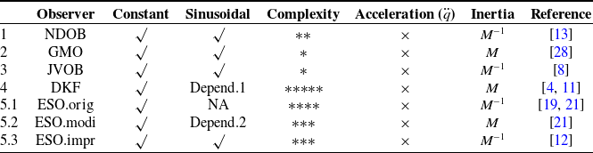
Note: Constant means constant disturbances; Sinusoidal means sinusoidal disturbances; Complexity means the subjective complexity of implementing the observers, and the more asterisk (*) means the more complexity of the implementation. Inertia means the form of the inertia matrix required.
Symbol (
 $\surd$
) means “yes, applicable”; NA, not applicable; symbol (
$\surd$
) means “yes, applicable”; NA, not applicable; symbol (
 $\times$
) means “no need.”
$\times$
) means “no need.”
Depend.1 means that it depends on what dynamics model of the disturbances is used. If a constant disturbance model is used, then it is only valid for constant disturbance, for example, a constant payload at the end-effector. If a polynomial disturbance model is used, then it is valid for both constant and time-varying disturbance.
Depend.2 means that it depends on parameter tuning. The same set of parameters cannot be valid for both constant and time-varying disturbances at the same time. The parameters need to be tuned separately in different disturbance scenarios in order for optimal effect in each.
Table VI shows that all the observers work for tracking constant disturbance. Only NDOB, GMO, JVOB, and ESO.impr work for tracking time-varying sinusoidal disturbances, while ESO.orig does not. For constant disturbances, the disturbance tracking error of observers can asymptotically converge to zero with different convergence speeds (see Fig. 17 for an example). For time-varying disturbances, the disturbance tracking error may not be able to converge to zero thus a bounded error may remain (see Fig. 19 for an example). Intuitively, this is because of that the observers need some time to converge to the target disturbance while some observers may need less time and some may need longer. If the target disturbance varies with respect to time, it may cause the observer not able to converge to zero in time and thus a bounded error. Theoretically, this is described in ref. [Reference Mohammadi, Tavakoli, Marquez and Hashemzadeh13] when the NDOB was developed, that is, for slow-varying disturbances, the disturbance tracking error of NDOB can converge asymptotically or exponentially to zero, while for fast-varying disturbances, the disturbance tracking error is globally uniformly ultimately bounded.
For using DKF to track the sinusoidal disturbances, it will depend on what disturbance model is used by the user. As introduced earlier, a disturbance model needs to be constructed by the user in the DKF method. If a constant disturbance model is used, then the DKF will only be valid for constant disturbances. If a polynomial disturbance model is used, then the DKF will be valid for both constant and sinusoidal disturbances. This is also reflected in the corresponding simulation results. For ESO.modi, it will depend on the parameter tuning result. For constant and sinusoidal disturbances, the observer gains may need to be tuned separately in each scenario in order to achieve optimal performance in each. Note that this is not necessary for NDOB, GMO, JVOB, and ESO.impr, for whom one set of observer gains work well for both constant and sinusoidal disturbances.
The complexity of implementing the observers is also subjectively ranked and presented in Table VI. Subjectively, GMO and JVOB are the easiest observers to be implemented, while DKF is the most complicated one. This can also be seen from the complex equations of DKF introduced earlier. It should note that the disturbance tracking performance of DKF is excellent although the complexity of implementation. Also, for ESO.orig and ESO.impr, there are three observer gains, which make them difficult to be tuned in order to find the optimal gain for best disturbance tracking performance.
There is no need for accelerations for all the presented observers, but some of them may need the inverse of the robot inertia matrix, including NDOB, JVOB, ESO.orig, and ESO.impr. For the specific NDOB design (7), the robot inertia matrix can be designed to be a positive definite diagonal matrix, for sure, which will introduce dynamic model error.
This paper is devoted to introducing all the required basics for implementing the five typical types of disturbance observers and presenting the possible behavior of each observer in the same simulated scenario for estimating the uncertainties in a robot control system. It is possible for the readers to quickly implement the introduced observers into a robot system relying on the information provided in this paper. Also, the presented simulation results can help to get an intuitive sense on the possible disturbance-tracking behavior of each observer in the same simulated scenario. At last, this study aims to help the users to better select the most suitable one for their own application scenario. Each observer has its own unique features; thus, has its own advantages in different application scenarios. It would be more meaningful to present the disturbance-tracking behaviors of different observers in the same simulated scenario, rather than to decide which one is superior to another, even though some may have better performance than others in a specific scenario.
Author contributions
TL and HX conceived and designed the study. TL conducted data gathering and analyses. TL, HX, EH, HT, and MT wrote the article.
Financial support
This research is supported in part by the Canada Foundation for Innovation (CFI) under grants LOF 28241 and JELF 35916, in part by the Government of Alberta under grants IAE RCP-12-021 and EDT RCP-17-019-SEG, in part by the Government of Alberta’s grant to Centre for Autonomous Systems in Strengthening Future Communities (RCP-19-001-MIF), in part by the Natural Sciences and Engineering Research Council of Canada (NSERC) under grants RTI-2018-00681, RGPIN-2019-04662, and RGPAS-2019-00106.
Competing interests
The authors declare no competing interests exist.
Ethical approval
Not applicable.
Supplementary material
The supplementary material for this article can be found at https://doi.org/10.1017/S0263574723001091


 Open access