


1. Introduction
Nowadays, data acquisition for 3D mapping can be automated by embedding sensors on mobile robots, reducing the need for human intervention [Reference Kim, Park, Cho and Kang1, Reference Tiozzo Fasiolo, Maset, Scalera, Macaulay, Gasparetto and Fusiello2]. Moreover, autonomous mobile platforms are suitable for environments inaccessible to humans, as well as in situations where the need for speed and simplicity outweighs the demand for accuracy. Additionally, when scanning systems are mounted on a mobile robot, their path is less susceptible to oscillations than when they are handheld. Smoother sensor paths may result in more accurate environmental reconstructions [Reference Maset, Scalera, Beinat, Visintini and Gasparetto3].
Mobile robotics could be useful in applications such as the digitalization of buildings and the creation of BIM models [Reference Ferguson and Law4]. BIM stands for Building Information Model and refers to the digital information system of the building: a 3D model integrated with the physical and functional data of the structure [Reference Volk, Stengel and Schultmann5]. Examples of mobile robots updating BIM models with new environmental elements can be found in the literature, as in [Reference Prieto, de Soto and Adan6]. Moreover, mobile robotic platforms are used to create BIM reconstructions of building interiors [Reference Adán, Quintana, Prieto and Bosché7] and exteriors [Reference Kim, Park, Cho and Kang1].
When using the Global Navigation Satellite System (GNSS) to reference the acquired data, denied satellite signals could lead to several-meter inaccuracies or to the inability to estimate coordinates. For this reason, GNSS receivers cannot be integrated into a mobile robotic platform to be used in mapping applications of building interiors. Furthermore, localization methods based solely on Inertial Measurement Units (IMUs) provide estimates of the motion of the robot that are insufficient for precise positioning in long surveys [Reference Segal, Haehnel and Thrun8].
For the reasons stated above, Simultaneous Localization and Mapping (SLAM) algorithms are required when using mobile scanning systems (e.g., mobile robots) for three-dimensional building reconstruction. These methods allow the sensor to be localized in an unknown environment while a map is being built. SLAM methods can be categorized into two main groups according to the types of data they rely on: visual-based [Reference Barros, Michel, Moline, Corre and Carrel9] and LiDAR-based [Reference Xu, Zhang, Yang, Cao, Wang, Ran, Tan and Luo10]. Visual-based algorithms retrieve the sensor pose by extracting characteristic features from images and recognizing these features in subsequent images. Moreover, visual-SLAM methods provide a three-dimensional representation of the environment by using stereo cameras, RGB-D sensors, or applying structure from motion with an image sequence [Reference Wang, Schworer and Cremers11, Reference Peng, Ma, Xu, Jia and Liu12]. However, in the latter case, the scale of the models is not determined automatically. On the other hand, LiDAR-based algorithms rely on the acquisition of subsequent scans that are properly registered to generate a point cloud of the environment. Due to the technical characteristics of the sensor, algorithms based on LiDAR data are the most suitable for 3D reconstruction. Indeed, LiDAR sensors can measure distances up to hundreds of meters, have a large field of view, directly provide 3D data, are not influenced by light conditions, and are less sensitive to surface characteristics.
LiDAR-based SLAM algorithms also exploit data from IMUs with the purpose of: (a) correcting potential point cloud distortions caused by the sensor motion during a single scan; (b) limiting errors in the registration of acquired point clouds during rapid movements of the sensor; (c) estimating the trajectory of the robot between consecutive acquisitions (since generally IMUs output data at a higher frequency than LiDAR sensors); and (d) helping in the convergence of the algorithms involved in assembling the acquired point clouds.
There are comparisons in the literature between point cloud reconstructions of buildings using commercial LiDAR-based SLAM algorithms and datasets collected using handheld mobile scanning devices [Reference Tucci, Visintini, Bonora and Parisi13]. However, the above-mentioned analyses do not involve open-source algorithms and datasets collected by autonomous mobile robots. On the other hand, developers of open-source LiDAR SLAM algorithms commonly conduct tests on open datasets such as KITTI [Reference Geiger, Lenz, Stiller and Urtasun14] (an urban environment), whereas other scenarios are less tested in the literature (e.g., indoor buildings with long corridors, courtyards with natural elements). Moreover, only the precision of the estimated trajectory is generally tested, and not the quality of the 3D reconstruction.
This paper proposes a comparison of open-source LiDAR and IMU-based SLAM approaches for 3D robotic mapping, building on [Reference Tiozzo Fasiolo, Scalera, Maset and Gasparetto15]. The work focuses only on algorithms that rely on standardized sensor data in order to use a single dataset for each test to guarantee the repeatability of results. Experimental tests are carried out using two different mobile robotic platforms in indoor and outdoor scenarios. The results compare the point clouds obtained with the different SLAM algorithms (with and without IMU data) in terms of density, accuracy, and noise.
The main contributions of this work with respect to [Reference Tiozzo Fasiolo, Scalera, Maset and Gasparetto15] are: (a) the comparison of SLAM algorithms based not only on LiDAR data but also on IMUs measurements; (b) the extension of the comparison with two additional algorithms that require mandatory IMU data fused with LiDAR in a coupled fashion; and (c) experimental tests with two different robotic platforms in both indoor and outdoor scenarios. The experimental results indicate the SLAM methods that are more suitable for 3D mapping in terms of the quality of the reconstruction and highlight the feasibility of mobile robotics in the field of autonomous mapping.
The paper is organized as follows: Section 2 recalls the compared LiDAR and IMU-based SLAM algorithms. Section 3 describes the experimental setup and the test cases. The experimental results are discussed in Section 4. Finally, Section 5 concludes the paper.
2. LiDAR and IMU-based SLAM algorithms
SLAM is the process of simultaneously estimating the location of a robotic system and generating a map of the surrounding area. The SLAM techniques can be divided into two main groups: filtering and smoothing [Reference Grisetti, Kümmerle, Stachniss and Burgard16]. In filtering approaches, the issue is tackled by incrementally estimating the state of the system, which consists of the current robot location and the map of the explored environment. Widespread filtering techniques are based on Kalman [Reference Montemerlo, Thrun, Koller and Wegbreit17] and particle [Reference Hahnel, Burgard, Fox and Thrun18] filters. Conversely, smoothing methods estimate the whole path of the robot and generally rely on least-square error minimization techniques [Reference Olson, Leonard and Teller19]. State-of-the-art smoothing methods address the SLAM problem via the formulation referred to as graph-based, first proposed in [Reference Lu and Milios20]. The graph-based SLAM involves the construction of a graph whose nodes represent robot poses or portions of the map, and edges embed the constraints between nodes (e.g., the relative transformation between two consecutive poses of the robot).
Generally, LiDAR SLAM algorithms estimate the path of the robot in two steps. The first step consists of performing a scan-to-scan alignment between adjacent LiDAR scans to recover an immediate motion guess. The second is to perform a scan-to-map registration between the current scan and the point cloud map of the environment to increase global pose consistency. During the scan-to-map stage, newly acquired points are added to the point cloud map [Reference Zhang and Singh27].
Consecutive LiDAR scans are first preprocessed to reduce the computational effort (e.g., via downsampling and feature extraction methods). The preprocessing also involves the correction of the point clouds, which are generally affected by the rotation mechanism of 3D LiDAR sensors and the motion of the sensor between two subsequent scans. Then, the scan-to-scan and scan-to-map registrations provide the updated map and the robot path. In addition, in smoothing LiDAR SLAM algorithms, path and map errors are minimized by using a graph-based formulation [Reference Madsen, Nielsen and Tingleff28].
In this work, the following state-of-the-art algorithms are considered: Real-Time Appearance-Based Mapping (RTAB-Map) [Reference Labbé and Michaud21], Lightweight and Ground-Optimized Lidar Odometry and Mapping (LeGO-LOAM) [Reference Shan and Englot22], LiDAR Inertial Odometry via Smoothing and Mapping (LIO-SAM) [Reference Shan, Englot, Meyers, Wang, Ratti and Rus23], hdl_graph [Reference Koide, Miura and Menegatti24], Direct LiDAR Odometry (DLO) [Reference Chen, Lopez, Agha-mohammadi and Mehta25], and Fast Direct LiDAR-Inertial Odometry (FAST-LIO2) [Reference Xu, Cai, He, Lin and Zhang26]. These algorithms are often exploited in mobile robotics for autonomous navigation since they output a six-degree-of-freedom pose with respect to a global reference frame. However, to the best of our knowledge, they are not often used for 3D building reconstruction.
The aforementioned algorithms were selected since they present: (a) distinct preprocessing and scan matching methodologies (the process of determining the relative transformation between two point clouds) that provide diverse outcomes in the final reconstruction; and (b) diverse structures for storing and accessing data throughout the mapping process, which might impact the computational efficiency of the algorithm. On the other hand, to speed up the calculations, each investigated algorithm (except for FAST-LIO2) performs a voxel downsampling of LiDAR scans. A voxel grid is an array of three-dimensional boxes over the point cloud data and, for data downsampling, all points in a voxel are approximated by their centroid.
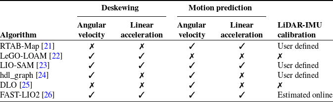
The main characteristics of the algorithms are listed in Table I, whereas the use of IMU data in each method is described in Table II. The LiDAR and IMU modules can work independently in SLAM algorithms with loose sensor fusion, but they are used together to compensate for the shortcomings of each distinct module. In contrast, SLAM algorithms with tight sensor fusion exploit both data sources simultaneously to provide a unique output. In the following, the algorithms compared in this paper are recalled.
Table I. Characteristics of the compared algorithms.
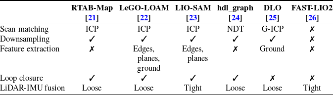
Table II. Applications of IMU in the compared algorithms.
2.1. RTAB-Map
RTAB-Map performs scan matching by using the Iterative Closest Point algorithm (ICP) on voxelized point clouds. In the ICP scan matching, the correlation between points of subsequent scans (or between the acquired scan and the point cloud map) is guessed based on a nearest-neighbor search [Reference Besl and McKay29]. More in detail, RTAB-Map uses a point-to-plane registration: in the nearest-neighbor search, it exploits the distance along the normals calculated on the acquired point cloud, instead of the Euclidean distance. The point-to-plane registration is preferred in scenarios characterized by planar surfaces [Reference Pomerleau, Colas, Siegwart and Magnenat30]. Moreover, before executing the scan-to-scan registration, a motion prediction is made according to a constant velocity model based on the previous path, or with an external motion guess (e.g., IMU-based). The motion prediction helps in avoiding completely wrong registrations and making the scan matching algorithm converge faster. The motion guess module accepts angular velocities and linear accelerations from an IMU to recover the poses of the LiDAR sensor during a scan. Moreover, a transformation matrix can be given as input to extrinsically calibrate the IMU and the LiDAR sensor.
Finally, once the scan-to-map registration is performed, RTAB-Map subtracts the global map from the acquired one and updates the map with the remaining points only. The motion of the robot during a
 $360^\circ$
scan can distort the acquired point cloud, since the map is generated by a rotating LiDAR sensor. If the angular velocity of the spinning LiDAR scanner is higher than the robot velocity, the distortion is limited [Reference Labbé and Michaud21]. Under this assumption, RTAB-Map neglects the distortion of the acquired scan.
$360^\circ$
scan can distort the acquired point cloud, since the map is generated by a rotating LiDAR sensor. If the angular velocity of the spinning LiDAR scanner is higher than the robot velocity, the distortion is limited [Reference Labbé and Michaud21]. Under this assumption, RTAB-Map neglects the distortion of the acquired scan.
2.2. LeGO-LOAM
LeGO-LOAM employs a scan matching approach based on a set of relevant points, instead of resorting to the whole downsampled point cloud. In particular, with a clustering process based on the Euclidean distance between neighboring points [Reference Bogoslavskyi and Stachniss31], LeGO-LOAM identifies points that relate to the same object or to the ground. The purpose of the clustering is to improve the search for correspondences between points. LeGO-LOAM distinguishes between points belonging to edges or planes [Reference Zhang and Singh27] and chooses a set of features to be used as input for the scan matching. The registration process proposed by LeGO-LOAM is tailored for ground robots. Indeed, it first computes the altitude, yaw, and pitch of the robot with a Levenberg–Marquardt optimization on the planar feature set. Subsequently, edge features are used to retrieve the robot pose on the plane in which it is navigating. Additionally, LeGO-LOAM exploits an ICP-based loop closure, which is the ability of recognizing if the mobile robot has returned to a previously visited location and of using this information to refine the map.
Furthermore, LeGO-LOAM accepts inputs from a 9-axis IMU sensor and calculates LiDAR sensor orientation by integrating angular velocity and linear acceleration readings in a Kalman filter. The measured point coordinates are then transformed and aligned with the orientation of the LiDAR sensor at the beginning of each scan. In addition, linear accelerations are used to adjust the robot motion-induced distortions in the recorded point cloud. The authors of LeGO-LOAM tested the algorithm with the integrated IMU of a Clearpath Husky mobile platform and did not furnish any information about the extrinsic calibration between IMU and LiDAR sensors [Reference Shan and Englot22]. If the IMU data are not provided, the undistortion of the acquired scan is performed assuming a linear motion model between consecutive scans.
2.3. LIO-SAM
Similarly to LeGO-LOAM, LIO-SAM performs an edge and plane feature extraction with the method in [Reference Zhang and Singh27]. In LIO-SAM, a 9-axis IMU is utilized to correct the distortions in the LiDAR scan and provide a motion prior to initialize the scan matching. Moreover, IMU data are also exploited to minimize the errors of the estimated path and map. The SLAM problem in LIO-SAM is modeled using a factor graph [Reference Dellaert and Kaess32] with three factors along with one state variable: the IMU preintegration factors, the LiDAR odometry factors, and the loop closure factors, with the pose of the robot as a variable. Thus, with the proposed method, the state estimation is formulated as a maximum a posteriori problem, which is equivalent to solving a nonlinear least-squares problem, assuming a Gaussian noise model in sensor readings [Reference Dellaert and Kaess32]. Finally, differently from LeGO-LOAM, LIO-SAM accepts a transformation matrix for LiDAR-IMU extrinsic calibration.
2.4. hdl_graph
hdl_graph exploits the Normal Distribution Transform (NDT) scan matching [Reference Biber and Strasser33]. NDT associates with each voxel a normal distribution that describes the likelihood of measuring a point over that cell. In this manner, it is possible to find the optimal transformation by maximizing the sum of the likelihood functions evaluated on the transformed points instead of performing ICP. The NDT is also used in hdl_graph for loop closure. Moreover, the ground plane and magnetometer orientation data are used as constraints to avoid drift along the
 $z$
axis due to the accumulated error. The motion prediction is performed by using angular velocities provided by the gyroscope while assuming a linear translational motion model.
$z$
axis due to the accumulated error. The motion prediction is performed by using angular velocities provided by the gyroscope while assuming a linear translational motion model.
More in detail, the motion prediction of hdl_graph is based on an Unscented Kalman Filter [Reference Wan and Van Der Merwe34], which allows the nonlinearities of the state transition model to be taken into account without linearizing the system as in the Extended Kalman Filter. The motion guess from the IMU is also used to correct the distortion in the acquired point cloud. Finally, hdl_graph considers an external calibration between IMU and LiDAR sensor reference frames.
2.5. DLO
DLO includes algorithmic features that favor computing speed and facilitate the usage of minimally preprocessed point clouds [Reference Chen, Lopez, Agha-mohammadi and Mehta25]. Indeed, it only exploits a voxel filter without extracting features. The scan matching is performed on a local submap point cloud instead of the whole map. Moreover, the registration is tackled with an ICP variant based on the Generalized-ICP [Reference Segal, Haehnel and Thrun8], in which a probabilistic model associating covariance matrices to points is added to the minimization step of the ICP. This formulation improves the convergence of the algorithm. However, the Generalized-ICP assumes that the environment is smooth and can be locally viewed as a plane. On the other hand, even if it performs scan matching similarly to the above-mentioned smoothing methods, DLO is not loop-closure capable since it is not a graph-based SLAM framework.
DLO accepts optional IMU data to perform motion prediction and to improve the correctness of the registration in the case of abrupt rotational motion of the mobile robot. However, only gyroscopic measurements found between the current LiDAR scan and the previous one are used. Moreover, through the first three seconds of measurements, during which the robot is assumed to be stationary, DLO calibrates the gyroscope online. Since the real value of the angular velocity, random noise, and bias are combined together in the gyroscope readings, estimating the bias increases the accuracy of motion prediction. However, DLO does not address the motion distortion of the obtained point cloud nor the LiDAR-IMU calibration.
2.6. FAST-LIO2
FAST-LIO2 directly registers the raw point cloud to the map without performing downsampling or feature extraction. The algorithms belongs to the category of filtering SLAM methods, and it is based on the tightly coupled iterated Kalman filter proposed in [Reference Xu and Zhang35]. More in detail, the state vector comprises IMU orientation and position, IMU velocity, as well as gyroscope and accelerometer biases (modeled as a random walk process). The state transition model is also used to compensate for each point motion during a
 $360^\circ$
scan of the LiDAR sensor, in the measurement model. Additionally, the measurement model removes the noise in range readings of the LiDAR sensor, leading to the measurement of the true point location in the sensor reference frame.
$360^\circ$
scan of the LiDAR sensor, in the measurement model. Additionally, the measurement model removes the noise in range readings of the LiDAR sensor, leading to the measurement of the true point location in the sensor reference frame.
In FAST-LIO2, the proposed Kalman filter consists of a forward propagation step upon each IMU measurement and an update step upon each LiDAR scan. Multiple propagation steps are usually performed before the update step, since IMU measurements are typically acquired at a higher frequency than LiDAR data. FAST-LIO2 not only accepts a user-defined LiDAR-IMU transformation matrix but is also capable of estimating calibration parameters online by including them in its state vector.
3. Material and methods
3.1. Mobile robots and sensors
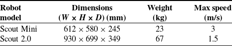
In this paper, two mobile robotic platforms by Agile-X Robotics are used for data collection (Fig. 1). The first is a Scout Mini, a compact and highly maneuverable robot (Fig. 1a). The second is a Scout 2.0, a larger mobile platform suited for outdoor applications (Fig. 1b). Both robotic platforms are provided with four independent electric motors. The specifications of the mobile platforms are reported in Table III.
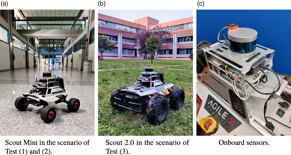
Figure 1. Mobile robots used for autonomous 3D mapping.
Table III. Specifications of the mobile platforms.
The mobile robots are equipped with a sensor suite (Fig. 1c), which features an NVIDIA Xavier computer (running Ubuntu 18.04 and ROS Melodic), a Velodyne VLP-16 LiDAR sensor, and an Xsens MTi-630 9-axis IMU, mounted on top of the LiDAR sensor. The position and orientation of the IMU and the LiDAR sensor are considered coincident in each test case (with an exeption for FAST-LIO2 that computes the extrinsic calibration matrix online).
The measurement range of the LiDAR sensor is 100 m, and it features 16 channels, a
 $360^\circ$
horizontal field of view, and a
$360^\circ$
horizontal field of view, and a
 $30^\circ$
vertical field of view (
$30^\circ$
vertical field of view (
 $\pm 15^\circ$
). The VLP-16 provides a vertical angular resolution of
$\pm 15^\circ$
). The VLP-16 provides a vertical angular resolution of
 $2^\circ$
, and a horizontal resolution of
$2^\circ$
, and a horizontal resolution of
 $0.2^\circ$
, as the rotation rate is set to 10 Hz. The accuracy is ±3 cm.
$0.2^\circ$
, as the rotation rate is set to 10 Hz. The accuracy is ±3 cm.
The IMU sensor comprises a gyroscope, an accelerometer, and a magnetometer. IMU direct measurements are fused together by an integrated Kalman filter, to provide linear accelerations, angular velocities, and the orientation of the sensor with respect to the magnetic north at 200 Hz. The specifications report a root-mean-square error of
 $0.25^\circ$
for roll and pitch, and
$0.25^\circ$
for roll and pitch, and
 $1^\circ$
for yaw.
$1^\circ$
for yaw.
Since the magnetic field of the Earth could be locally distorted due to the presence of currents and ferromagnetic materials on the robot, a calibration of the magnetometer is needed to compensate for the iron effects. This calibration is performed with the Magnetic Field Mapper software by Xsens.
The robots are autonomous in navigation thanks to the development of a custom navigation framework described in Fig. 2. Since in previous tests [Reference Tiozzo Fasiolo, Scalera, Maset and Gasparetto15] DLO demonstrated to be a suitable and computationally light source of odometry, it has been chosen as the localization method for robot navigation. Moreover, to provide suitable information on the environment for path planning, a bi-dimensional map is created and continuously updated online with the GMapping algorithm [Reference Grisetti, Stachniss and Burgard36]. The LiDAR points falling within a predefined height range are projected on a plane to provide a bi-dimensional scan that can be used by GMapping via the pointcloud_to_laserscan ROS module (P2L). The collision-free path between the way points is calculated with the Dijkstra algorithm. The path can be modified online in case of potential collisions with obstacles by means of the dynamic window approach (DWA).
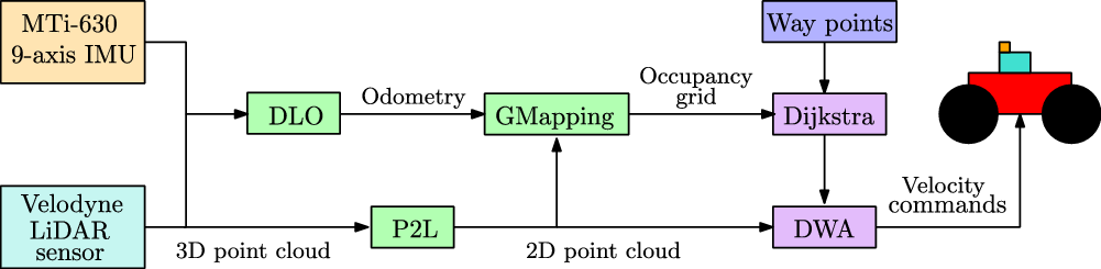
Figure 2. Architecture of the navigation framework.
During each autonomous survey, the robots collect raw data from sensors in the file format called ROS Bags. Reproducing ROS Bags files replicate the sensors transmitting identical data at the same rate they were recorded. Subsequently, the aforementioned SLAM algorithms are executed, utilizing the ROS Bags as input, on a workstation equipped with 32 GB RAM and an Intel Core i9 processor, running Ubuntu 18.04 and ROS Melodic.
The ground-truth for the indoor scenario is acquired with a RIEGL Z390i terrestrial laser scanner (TLS). The instrument relies on the time-of-flight measurement principle, featuring respectively a
 $360^\circ$
and a
$360^\circ$
and a
 $80^\circ$
horizontal and vertical field of view, with an angular step of
$80^\circ$
horizontal and vertical field of view, with an angular step of
 $0.1^\circ$
. The declared accuracy in range measurements is 6 mm, with a repeatability of 4 mm for single shots and 2 mm for averaged measures. For the outdoor case, the ground-truth map is retrieved by means of a Leica BLK360 G1 TLS. This TLS has a
$0.1^\circ$
. The declared accuracy in range measurements is 6 mm, with a repeatability of 4 mm for single shots and 2 mm for averaged measures. For the outdoor case, the ground-truth map is retrieved by means of a Leica BLK360 G1 TLS. This TLS has a
 $360^\circ$
and a
$360^\circ$
and a
 $300^\circ$
horizontal and vertical field of view, respectively. The measurement range is 0.6 ÷ 60 m, whereas the accuracy in range measurements (for a surface with
$300^\circ$
horizontal and vertical field of view, respectively. The measurement range is 0.6 ÷ 60 m, whereas the accuracy in range measurements (for a surface with
 $78\%$
albedo) is 4 mm at 10 m, and 7 mm at 20 m.
$78\%$
albedo) is 4 mm at 10 m, and 7 mm at 20 m.
3.2. Experimental test cases
Three experiments are conducted in the main building of the scientific campus of the University of Udine (Italy), in both indoor and outdoor areas:
-
Test (1) is performed in a single corridor of the west wing of the building (40 m long, 8 m wide, and 4 m high) to evaluate the point clouds of an indoor environment in terms of points density and accuracy;
-
Test (2) is performed in the whole squared plant of the west wing of the building (80 × 80 m, measured along the center line of the corridors) to evaluate accumulated errors in a long survey, during which new and unknown portions of the building are explored;
-
Test (3) is performed in one of the courtyards inside the building (45 × 45 m, measured along the center line of the external corridors) to evaluate the noisiness of the point clouds of an outdoor environment and the accumulated errors.
The data acquisition is performed by the Scout Mini (Fig. 1a) in Test (1) and (2) and by the Scout 2.0 (Fig. 1b) in Test (3). The indoor environments of Test (1) and (2) can be considered structured as they are characterized by the presence of planes. Corridor-like environments can cause localization errors and misaligned scan registration if an approximate motion guess (between subsequent scans) is not provided (e.g., from an IMU). In contrast, the surroundings in Test (3) are less structured and present some natural characteristics (e.g., trees). Moreover, the grounds on which the robots navigate are different, since in Test (1) and (2) the floor is planar, whereas in Test (3) the robot moves on grass and tiles, causing jerking or sudden movements of the LiDAR sensor that cannot be described by a linear motion.
To determine the impact of the IMU sensor on map quality, experiments are conducted with and without IMU data for algorithms with loose IMU integration (RTAB-Map, LeGO-LOAM, and hdl_graph, DLO). On the other hand, IMU is always required in LIO-SAM and FAST-LIO2.
Each dataset is acquired by the robot while moving through 5-way points in Test (1), 9-way points in Test (2), and 9-way points in Test (3). Each way points set defines a closed path inside the environment. On the other hand, the ground-truth model of Test (1) is acquired by placing the TLS at three different positions (distant 12.5 m from each other) along the centerline of the corridor, exploiting as tie points reflecting disks and cylinders distributed on the floor and walls to register the individual point clouds. The reference map for Test (3) is obtained thanks to 12 scans, merged together by the targetless registration algorithm implemented in Leica Cyclone Register 360 software.
4. Experimental results
This section reports the experimental results and the comparison between the considered SLAM algorithms. Discussions on surface density, point distributions, and accuracy are reported in Section 4.1. Furthermore, the influence of loop closure in the minimization of accumulated errors is discussed in Section 4.2. Finally, Section 4.3 reports point cloud noise measurements. In the following, the * indicates the use of both LiDAR and IMU data.
4.1. Results of Test (1)
The first evaluation considers the surface density of the point cloud in the indoor environment of Test (1). The reason is that as the number of points increases, so does the ability of the point cloud to characterize the environment in terms of geometry variations. The absolute number of points and density obtained by means of each algorithm are reported in the first and second columns of Table IV, respectively.
Table IV. Experimental results of Test (1): total number of points, surface density, and C2C absolute distances from the ground-truth point cloud. The * indicates the use of both LiDAR and IMU data.
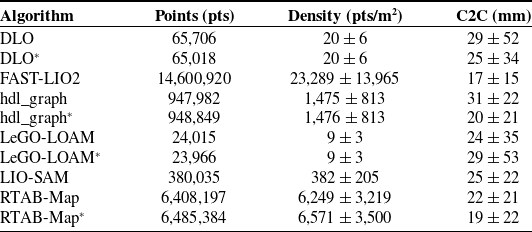
The best results in terms of surface density are obtained by using FAST-LIO2 (23,289 ± 13,965 pts/m2). Indeed, FAST-LIO2 is the only algorithm capable of processing the whole acquired scan without the need for downsampling. On the other hand, among the algorithms that process the cloud with a voxel filter, the best results are obtained with RTAB-Map, followed by hdl_graph.
A visual representation of the point clouds is shown in Fig. 3. The contour plots indicate regions with higher surface density and regions where the point cloud is sparser. DLO (Fig. 3a) and LeGO-LOAM (Fig. 3d) provide point clouds with too low density for 3D mapping. In fact, only the principal geometric components of the corridor (such as walls and floors) are recognized. On the other hand, in FAST-LIO2 (Fig. 3b), hdl_graph (Fig. 3c), LIO-SAM (Fig. 3e), and RTAB-Map (Fig. 3f) variations in geometry and characteristics of the environment are more prominent, making them suitable for 3D mapping.
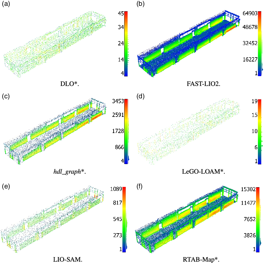
Figure 3. Contours of the surface density (pts/m2) for Test (1). The * indicates the use of both LiDAR and IMU data.
Histograms of surface density for Test (1) are shown in Fig. 4. The single peaks in histograms of DLO (Fig. 4a and b) and LeGO-LOAM (Fig. 4f and g) indicate that the point distribution in the reconstruction is rather regular. This may be associated with the use of a voxel filter in the final point cloud. In contrast, the histograms of FAST-LIO2 (Fig. 4c), hdl_graph (Fig. 4d and e), LIO-SAM (Fig. 4h), and RTAB-Map (Fig. 4i and j) present two peaks. This is related to the horizontal installation of the LiDAR sensor on top of the robot along with its vertical resolution. Thus, walls get the highest density, but the ground surface has a low density.
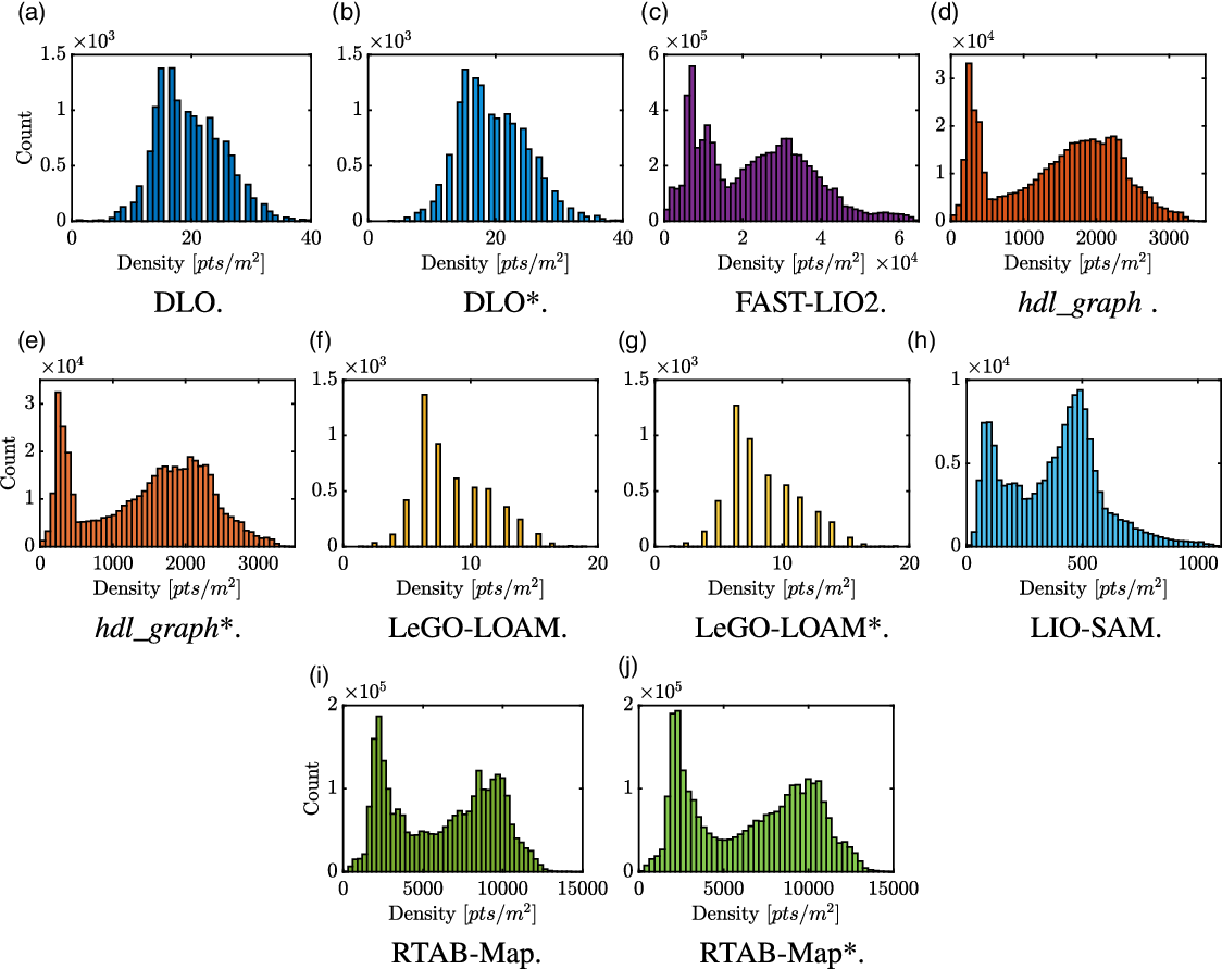
Figure 4. Histograms of surface density for Test (1). The * indicates the use of both LiDAR and IMU data.
Subsequently, the accuracy and precision of the point clouds are examined. The metric used in the evaluation is the cloud-to-cloud absolute distance (C2C) with respect to the ground-truth model (acquired by means of the TLS). A box plot representation of the C2C results is shown in Fig. 5, whereas the mean values and standard deviations of the C2C absolute distances are reported in Table IV.
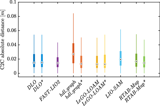
Figure 5. Box plots of C2C absolute distance.
In the indoor scenario of Test (1), FAST-LIO2, which is a tightly coupled LiDAR-IMU SLAM algorithm, is the best choice in terms of C2C absolute distance. Moreover, the use of IMU leads to an improvement in the point cloud accuracy for the algorithms that adopt a loose sensor fusion method (except for LeGO-LOAM). In hdl_graph, the use of angular velocities leads to a
 $35\%$
decrease in C2C mean value, while reducing the standard deviation. In contrast, integrating IMU data in LeGO-LOAM degrades the C2C results leading to an increase of
$35\%$
decrease in C2C mean value, while reducing the standard deviation. In contrast, integrating IMU data in LeGO-LOAM degrades the C2C results leading to an increase of
 $21\%$
in the mean value and of
$21\%$
in the mean value and of
 $51\%$
in the standard deviation.
$51\%$
in the standard deviation.
Additional analyses are conducted through a visual inspection of the point clouds. It can be noticed that DLO presents some misaligned single scans when relying on LiDAR data only. With the additional use of the IMU sensor, this problem is limited. On the other hand, in LeGO-LOAM, more inconsistent points appear when using the IMU. It is worth noting that, since the total amount of points of LeGO-LOAM is low, the computed C2C values may be affected by these outliers. Similar problems arise with RTAB-Map when relying on IMU data. More in detail, a large number of irregular points appear on the ground surface. This may be related to noise in linear acceleration signals that are used by LeGO-LOAM and RTAB-Map. In addition, many individual scans in RTAB-Map are often misplaced, with points far from the walls.
Noise also appears in the point clouds generated by FAST-LIO2. In addition, in FAST-LIO2, badly registered scans at the end of the corridor, where the robot changes direction, produce plenty of inconsistent points (Fig. 6a). In contrast, the point clouds provided by hdl_graph present low noise and few outliers on the walls, both using LiDAR only and the additional IMU data (Fig. 6b), a behavior visible also in the result obtained by LIO-SAM. As expected, in most algorithms, it is noticeable that at the end of the corridor, that is, in the areas mapped while the robot is performing a U-turn, there are poorly registered scans.
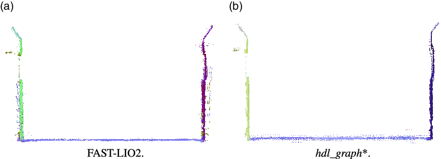
Figure 6. Vertical section of the point clouds at the end of the corridor. Badly registered scans are visible in the FAST-LIO2 result (a), whereas hdl_graph* presents low noise on the walls (b).
4.2. Results of Test (2)
Test (2) consists of mapping the whole squared plant of the west wing of the considered building, composed of four corridors, as shown in Fig. 7. Performing a closed loop, the area at the beginning and at the end of the path is surveyed twice, and drift accumulated along the trajectory can lead to doubled surfaces, that is, the same geometric element appears twice in the map due to residual misalignment. For this reason, a measure of the distance between these elements is valuable to quantify the accumulated error in the final map. To facilitate distance measurements on the
 $xy$
plane and
$xy$
plane and
 $z$
direction, X-ray orthophotos are retrieved from the point clouds shown in Fig. 7 by projecting the points on the horizontal and vertical plane, respectively. In the orthophotos, duplicated geometries result in distinct segments between which sample distances are measured to compute an average value. The average value of accumulated drift along each of the three axes is shown in Table V. The
$z$
direction, X-ray orthophotos are retrieved from the point clouds shown in Fig. 7 by projecting the points on the horizontal and vertical plane, respectively. In the orthophotos, duplicated geometries result in distinct segments between which sample distances are measured to compute an average value. The average value of accumulated drift along each of the three axes is shown in Table V. The
 $x$
-axis is aligned with the middle line of the corridor of Test (1), whereas the
$x$
-axis is aligned with the middle line of the corridor of Test (1), whereas the
 $z$
-axis is orthogonal to the ground plane.
$z$
-axis is orthogonal to the ground plane.

Figure 7. Point clouds obtained for Test (2). The * indicates the use of both LiDAR and IMU data. The green dot, the red dots, and the arrow indicate the starting and ending way point, the way points, and the direction of the robot motion, respectively.
Table V. Experimental results of Test (2): accumulated errors in correspondence of the loop closure. The * indicates the use of both LiDAR and IMU data.
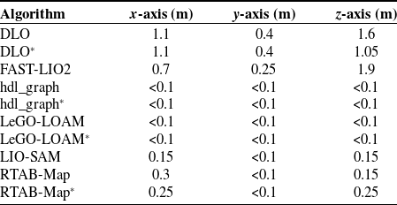
Algorithms not exploiting loop closure and graph optimization (DLO and FAST-LIO2) show not to be suitable for long surveys. On the other hand, the best results are obtained with hdl_graph and LeGO-LOAM, which are smoothing SLAM methods with loop closure. These two algorithms provide 3D maps with small errors that are in the order of magnitude of the pixel dimension of the orthophoto (with and without IMU data). As an example, the point clouds at the loop closure obtained by FAST-LIO2 and hdl_graph* are shown in Fig. 8. Due to the high drift error along the
 $z$
direction that affects FAST-LIO2, the floor appears doubled in Fig. 8a.
$z$
direction that affects FAST-LIO2, the floor appears doubled in Fig. 8a.

Figure 8. Point clouds at the loop closure.
It is worth noting that hdl_graph assumes the environment has a single-level floor and optimizes the pose graph such that the ground plane observed in every single scan is the same. Without the plane constraint, the final point cloud presents a large drift along the
 $z$
-axis due to the accumulated rotational error [Reference Koide, Miura and Menegatti24]. Thus, this method is unsuitable if the environment presents changes in level. In general, the use of IMU data leads to a decrease in the accumulated error along each axis for all the algorithms. In particular, using angular velocities in DLO results in a reduction of the accumulated error along the
$z$
-axis due to the accumulated rotational error [Reference Koide, Miura and Menegatti24]. Thus, this method is unsuitable if the environment presents changes in level. In general, the use of IMU data leads to a decrease in the accumulated error along each axis for all the algorithms. In particular, using angular velocities in DLO results in a reduction of the accumulated error along the
 $z$
-axis of the 34%. RTAB-Map is an exception, since the additional use of IMU slightly increases the drift along the
$z$
-axis of the 34%. RTAB-Map is an exception, since the additional use of IMU slightly increases the drift along the
 $z$
-axis.
$z$
-axis.
4.3. Results of Test (3)
The reconstructions of the outdoor courtyard of Test (3) are shown in Fig. 9. In this scenario, each algorithm provides a point cloud devoid of accumulated drift, except for hdl_graph, which presents visible deformations in the facade of the building surveyed at the beginning and at the end of the trajectory.
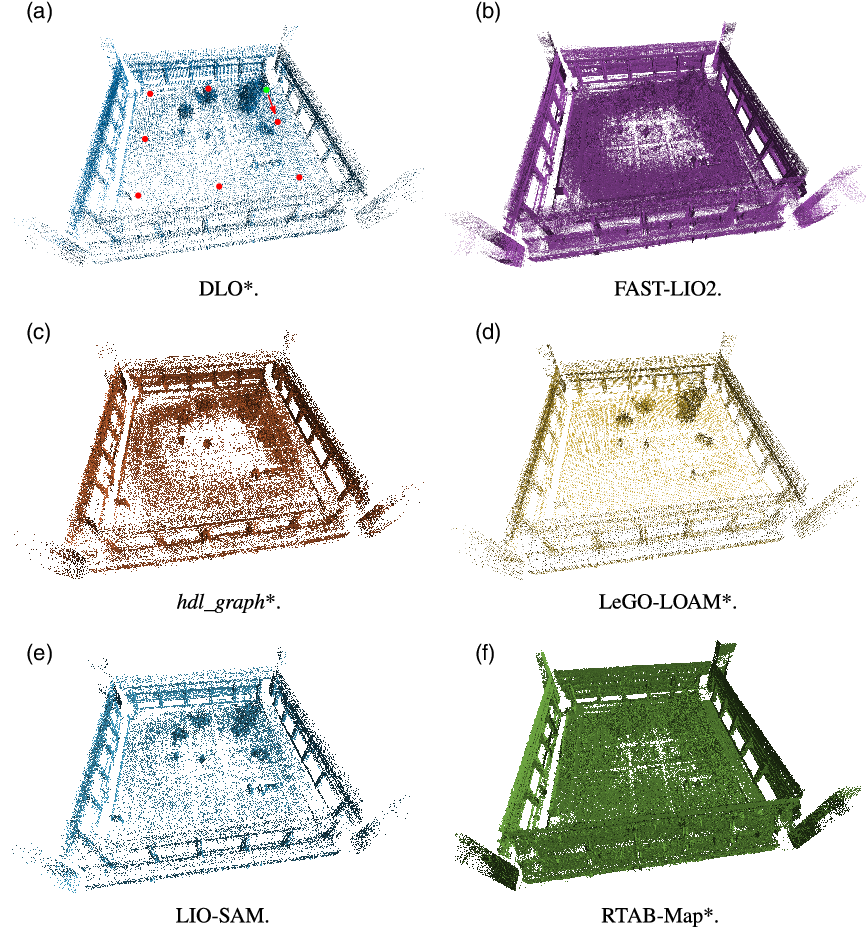
Figure 9. Point clouds obtained for Test (3). The * indicates the use of both LiDAR and IMU data. The green dot, the red dots, and the arrow indicate the starting and ending way point, the way points, and the direction of the robot motion, respectively.
To provide a quantitative evaluation of the noisiness of the 3D map, the roughness is used as a metric. For each point, the roughness value is equal to the distance between this point and the best-fitting plane computed on its nearest neighbors. Only the nearest neighbors that fall within a predefined euclidean distance from the point are considered. If there are not enough neighbors to estimate the plane by means of the least squares fitting (i.e., less than 3), it is not possible to compute the roughness. For this reason, it is difficult to assess point clouds with a too-low density.
The obtained roughness values are reported in Table VI, computed for a single facade using a neighboring radius of 0.3 m. FAST-LIO2 provides the best results (22 ± 30mm). Moreover, in this scenario, the drift accumulated by this algorithm is lower than in Test (2). However, there are many scans not properly registered and a high number of outlier points. This issue occurs most often in areas of the environment scanned when the robot is changing direction.
Table VI. Experimental results of Test (3): point cloud roughness on a portion of the building facade. The * indicates the use of both LiDAR and IMU data.
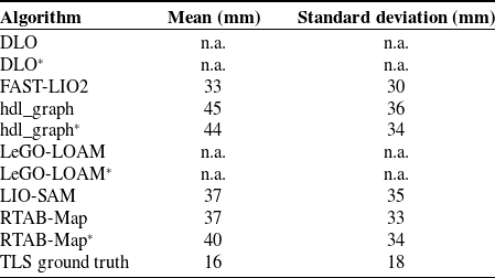
The evaluation of roughness in point clouds provided by DLO and LeGO-LOAM is meaningless given their low density. However, via a visual inspection of points belonging to walls, it can be noticed that noise is considerably reduced by means of the IMU integration, especially in DLO. On the other hand, RTAB-Map provides the densest reconstruction and a few numbers of bad registered scans. However, the extra use of IMU data increases the noisiness (roughness increased by
 $8\%$
). Given its reasonable point cloud surface density and the limited number of outliers, the reconstruction provided by LIO-SAM can be considered the best trade-off in this scenario.
$8\%$
). Given its reasonable point cloud surface density and the limited number of outliers, the reconstruction provided by LIO-SAM can be considered the best trade-off in this scenario.
5. Conclusion
In this paper, we proposed a comparison of open-source LiDAR and IMU-based SLAM approaches for 3D robotic mapping. Experimental tests have been carried out using two different autonomous mobile platforms in three test cases comprising both indoor and outdoor scenarios. The point clouds obtained with the different SLAM algorithms have been then compared in terms of density, accuracy, and noise of the point clouds to analyze the performance of the different approaches.
As expected, the quality of the reconstruction varies with the characteristics of the environment. More in detail, the indoor scenario is more critical for the scan matching. This is related to the presence of long corridors and repetitive geometrical elements. Indeed, the lack of distinctive traits often causes drift accumulation. For this reason, methods that do not exploit loop closure demonstrate to be not suitable for long surveys, especially in this environment.
On the other hand, the courtyard is an environment with higher variability and more changes in the geometry of its elements. Moreover, there is a higher overlapping of scans even for portions of the environment scanned from positions far apart. This considerably helps the scan matching. However, the irregularities of the terrain in which the robot navigates make the exploitation of IMU signals more critical, resulting in a higher number of outliers and bad registered scans. From this point of view, among the algorithms with loose sensor fusion, the use of the IMU data implemented in DLO seems to be the approach that better increases the results with respect to the case without IMU.
Tightly-coupled systems (i.e., LIO-SAM and FAST-LIO2) offer improved accuracy with respect to loosely coupled LiDAR-inertial SLAM methods. More in detail, FAST-LIO2 provides suitable results for mapping purposes in environments of small dimensions in which there is a great overlay between scans. However, as it lacks strategies for global map correction, a large accumulation of errors appears in long surveys. This problem could be solved by integrating loop closure and LiDAR bundle adjustment [Reference Liu and Zhang37]. By the way, it is the algorithm providing the higher surface density. On the other hand, considering both the indoor and outdoor test, LIO-SAM, which tightly integrates LiDAR and IMU data by means of a factor graph, is the best trade-off between surface density and the accuracy of the reconstruction.
Future works will include the application of the more promising algorithms found in this paper to other scenarios, such as agricultural environments. Furthermore, in the future, we plan to integrate additional sensors, such as GNSS, to improve the navigation and the quality of the reconstruction in outdoor 3D mapping.
Author contributions
All authors contributed to the study conception and design. DTF conducted data gathering, and EM performed data analysis. The first draft of the manuscript was written by DTF. All authors commented and read the manuscript.
Financial support
This research has been developed within the Laboratory for Big Data, IoT, Cyber Security (LABIC) funded by Friuli Venezia Giulia region, and the Laboratory for Artificial Intelligence for Human-Robot Collaboration (AI4HRC) funded by Fondazione Friuli.
Conflicts of interest
The authors declare no conflicts of interest exist.
Ethical approval
Not applicable.


 Open access