


Discordant monozygotic (MZ) twin methods can produce estimates unconfounded by genetic and shared environmental factors that is unrivaled by many other statistical methodologies (Oskarsson et al., Reference Oskarsson, Thisted Dinesen, Dawes, Johannesson and Magnusson2017; Ross et al., Reference Ross, Ellingson, Rhee, Hewitt, Corley, Lessem and Friedman2020; Tiu et al., Reference Tiu, Wadsworth, Olson and DeFries2004; Vitaro et al., Reference Vitaro, Brendgen and Arseneault2009). Since MZ twins share 100% of their genetic material and 100% of their shared environment, it can be assumed that any phenotypic differences between MZ twins correspond to divergent environmental factors (i.e., the nonshared environment; Knopik et al., Reference Knopik, Ndiderhiser, DeFries and Plomin2016). As such, relative to standard social science models, the confidence in the estimates is substantively increased through the use of discordant MZ twin methods because it can be assumed that genetic and shared environmental factors are constant across MZ twins (Vitaro et al., Reference Vitaro, Brendgen and Arseneault2009). Unobserved heterogeneity in the genome, phenotypic characteristics and shared environmental factors are adjusted for when using discordant MZ twin methods due to the co-twin establishing a robust counterfactual condition with genetic and shared environmental experiences identical to the target twin (Knopik et al., Reference Knopik, Ndiderhiser, DeFries and Plomin2016).
Discordant MZ methods permit evaluation of the associations between nonshared environmental factors and phenotypic variation without the collection of molecular genetic information (e.g., single-nucleotide polymorphisms [SNPs]), information pertaining to shared phenotypes or information on the shared environment (Knopik et al., Reference Knopik, Ndiderhiser, DeFries and Plomin2016). Moreover, the estimates produced by discordant MZ analyses can be adjusted for observed heterogeneity in discordant nonshared environmental factors (i.e., factors that differ between the twins; Knopik et al., Reference Knopik, Ndiderhiser, DeFries and Plomin2016). Given the capacity to estimate effects with limited biases, discordant MZ twin methods are commonly used in the behavioral and social sciences and are considered robust analytical tools for evaluating causal associations at the individual level (e.g., Asbury et al., Reference Asbury, Dunn, Pike and Plomin2003; Motz et al., Reference Motz, Barnes, Caspi, Arseneault, Cullen, Houts, Wertz and Moffitt2019; Oskarsson et al., Reference Oskarsson, Thisted Dinesen, Dawes, Johannesson and Magnusson2017; Silberg et al., Reference Silberg, Copeland, Linker, Moore, Roberson-Nay and York2016; Thornton et al., Reference Thornton, Trace, Brownley, Ålgars, Mazzeo, Bergin, Maxwell, Lichtenstein, Pedersen and Bulik2017). Nevertheless, large cohorts of molecular genetic data, such as the UK Biobank, and the advancement of polygenic risk scores (PRSs) provide the ability to reduce observed genetic risk information and environmental information to a single score, potentially presenting an opportunity to match the estimates produced by discordant MZ twin methodologies using singletons.
Given the availability of molecular genetic data and advanced techniques, an alternative procedure intended to produce results similar to discordant MZ twin methods is discussed in the current study. This alternative procedure — termed genetically adjusted propensity scores (GAPS) — integrates polygenic scores into the calculation of a propensity score to adjust for the confounding effects of genetic and environmental factors on an association of interest through matching. The GAPS matching methodology and the results from various simulated analyses are presented. These results are intended to provide an indication of the conditions necessary for GAPS matching to estimate associations within the confidence intervals of discordant MZ twin methods. Furthermore, a thorough discussion of the benefits and challenges associated with GAPS matching is provided to emphasize the validity of the methodology. GAPS matching integrates both propensity scores (created from observed environmental measures) and polygenic scores (created from observed genetic SNPs) to adjust for the confounding influence of genetic and environmental factors on associations of interest.Footnote 1
Propensity Score Matching
Briefly, a propensity score is defined as the probability of being exposed to a treatment given the phenotype of an individual and their environmental circumstances (Guo & Fraser, Reference Guo and Fraser2015). Footnote 2 A propensity score can be estimated using a variety of generalized linear models, conditional upon the level of measurement of the treatment, with a binary logistic regression model being the most common (Guo & Fraser, Reference Guo and Fraser2015). As displayed in Eq. 1, a propensity score ( P ) is the exponential value of a case’s weighted scores ( β ) on the matrix of independent variables ( X i ), divided by 1 plus the exponential value of a case’s weighted scores ( β ) on the matrix of independent variables ( X i ). The weights ( β ) are derived from regressing the logged odds of the treatment ( v i ; 0 = not exposed to treatment; 1 = exposed to treatment) on the matrix of independent variables ( X i ):
 $$\log ({{{{\bf{v}}_i}} \over {1 - {{\bf{v}}_i}}}) = {\beta}{{\bf{X}}_{\bf{i}}} + \varepsilon $$
 $${\bf{P}} = {{\exp ({\bf{\beta }}{{\bf{X}}_i})} \over {1 + \exp {\beta}{{\bf{X}}_i}}}$$
Propensity scores can be employed in various ways to reduce the bias in the estimated effects of a treatment on an outcome of interest. A frequently used method is propensity score matching, which is a technique designed to emulate an experimental condition by matching treatment cases to control cases with a similar probability of being exposed to the treatment (i.e., propensity score; Guo & Fraser, Reference Guo and Fraser2015). Treatment cases and control cases can be matched using various techniques, of which the most easily understood are exact matching (Eq. 2) and caliper matching (Eq. 3; ϵ represents the caliper):
 $${{\bf{P}}_{(t comma = comma 1)}} = {{\bf{P}}_{(t comma = comma 0)}}$$
 $$\left\| {{{\bf{P}}_{(t comma = comma 1)}} - {{\bf{P}}_{(t comma = \ 0)}}} \right\| \lt comma \varepsilon $$
Propensity score matching, as well as other propensity score techniques, are beneficial under conditions where the phenotypic traits and environmental circumstances that influence exposure to the treatment can be directly measured (Guo & Fraser, Reference Guo and Fraser2015). However, where some or all of the phenotypic traits and environmental circumstances influencing exposure to the treatment cannot be directly measured, the applicability of propensity score techniques is limited (Guo & Fraser, Reference Guo and Fraser2015). Moreover, in addition to the assumptions of a generalized linear regression model (e.g., linearity, normality and heteroscedasticity; Fox, Reference Fox2016), propensity score matching requires the satisfaction of the assumption of common support and covariate balance (Guo & Fraser, Reference Guo and Fraser2015). Common support refers to the assumption that the distribution of the covariates across the treatment and control groups are similar enough to permit matching, while covariate balance refers to the assumption that the similarity in the distribution of the covariates across the treatment and control groups is improved through matching (Guo & Fraser, Reference Guo and Fraser2015). These assumptions are fundamental to conducting propensity score matching, as limited common support generates difficulties matching and limited covariate balance reduces the ability to emulate experimental conditions (Guo & Fraser, Reference Guo and Fraser2015).
Polygenic Risk Scores
A PRS is an estimate of the effects of multiple alleles on a phenotype, designed to approximate the cumulative genetic likelihood — that is, risk — of an individual experiencing a phenotype. The calculation of a PRS begins with subjecting an independent dataset containing information about the participant’s SNPs to a genomewide association study (GWAS; Dudbridge, Reference Dudbridge2013).
Footnote 3
A GWAS regresses the phenotype of interest on each SNP using a generalized linear model. The estimated effects of each SNP (βj) from the independent GWAS is then used to estimate the genetic likelihood of experiencing the phenotype in the dataset of interest. This estimate is created using Eq.4, where the raw polygenic score (PRS
i
) is equal to the aggregated value of the coefficient of (βj) multiplied by the number of reference alleles that individual (i) possesses (
G
ij
). The PRS
i
can then be transformed to produce the respondents’ standardized polygenic scores (
 ${z_{{\bf{PRS}}}}_{_i}$
). Importantly, PRSs are assumed to only represent the additive genetic risk for a phenotype and cannot be used to provide an indication of other genetic processes (e.g., dominant, epistasis and epigenetic risk; Dudbridge, Reference Dudbridge2013; Euesden et al., Reference Euesden, Lewis and O’Reilly2015). Moreover, PRSs can be calculated using only SNPs that reach a prespecified statistical threshold (typically, 0.05 * 10–6), or using the whole genome (Francisco & Bustamante, Reference Francisco and Bustamante2018):
${z_{{\bf{PRS}}}}_{_i}$
). Importantly, PRSs are assumed to only represent the additive genetic risk for a phenotype and cannot be used to provide an indication of other genetic processes (e.g., dominant, epistasis and epigenetic risk; Dudbridge, Reference Dudbridge2013; Euesden et al., Reference Euesden, Lewis and O’Reilly2015). Moreover, PRSs can be calculated using only SNPs that reach a prespecified statistical threshold (typically, 0.05 * 10–6), or using the whole genome (Francisco & Bustamante, Reference Francisco and Bustamante2018):
 $${\bf{PR}}{{\bf{S}}_i} = \sum\limits_{j comma = comma 1}^m {{\beta}_j}{{\bf{G}}_{ij}} $$
Given that the estimates from a GWAS are fundamental to the calculation of a PRS, the estimated likelihood is subject to missing heritability. Briefly, while labeled as missing heritability, the concept refers to the difference in the variance explained by genetic factors between ACE decomposition models and GWAS. In general, a GWAS produces heritability estimates substantially smaller than ACE decomposition models, suggesting that GWAS cannot explain the variation in a phenotype as well as twin-based models. The missing heritability concept has important implications when discussing PRSs, as the variation in a PRS cannot predict the variation in a phenotype as well as the difference between MZ twins. For instance, a PRS predicts the variance in a phenotype substantially worse than a MZ difference score under conditions where the heritability estimate from a twin study indicates that 60% of the variance in a phenotype is attributed to genetics (h 2 = .60), but a GWAS indicates that only 10% of the variance in the phenotype is attributed to genetics (r 2 = .10). While suggested to be a function of the number of parameters compared to the sample size, missing heritability has important implications for the GAPS matching approach.
Genetically Adjusted Propensity Score (GAPS) Matching
Similar to propensity and PRS, GAPS matching was designed as a data reduction technique intended to capture respondents’ observed genetic and environmental risk for a phenotypic outcome of interest. A GAPS can be calculated by combining respondents’ polygenic scores with respondents’ propensity scores and removing any covariation between the terms. The combination of the polygenic score and propensity score can be achieved by introducing the polygenic score (as an independent variable) into the regression analysis used to calculate the propensity score. Although a variety of models can be used to estimate propensity scores (Guo & Fraser, Reference Guo and Fraser2015), calculating GAPS for dichotomous constructs provides a straightforward example of the estimation procedure. After calculating and standardizing a PRS, a generalized linear model can be estimated to create a GAPS (Guo & Fraser, Reference Guo and Fraser2015). For example, a logistic regression model could be estimated, where the log-odds of a dichotomous variable (identified as
v
) would be regressed on the polygenic score and measures of environmental constructs. This process is captured in Eq. 5, where
v
i
represents a dichotomously measured outcome variable,
 ${{\bf{Z}}_{PR{S_i}}}$
represents a m × n matrix of standardized PRSs (one or more polygenic scores can be included in the estimation procedure), and X
ki
represents a m × n matrix of environmental constructs:
${{\bf{Z}}_{PR{S_i}}}$
represents a m × n matrix of standardized PRSs (one or more polygenic scores can be included in the estimation procedure), and X
ki
represents a m × n matrix of environmental constructs:
 $$\log ({{{{\bf{v}}_i}} \over {1 - {{\bf{v}}_i}}}) = {\beta}{{\bf{Z}}_{{PRS_i}}} + {\bf{\beta}}{X_i}$$
After calculating the slope coefficients (
β
), Eq. 3 is used to calculate the GAPS. As demonstrated by Eq. 6, GAPS (#xi;
i
) is equal to the exponential value (exp) of a participant’s weighted scores on the independent variables (
 ${\beta}{{\bf{Z}}_{PR{S_i}}} + {\beta}{X_i}$
divided by 1 + the exponential value of a participant’s weighted scores on the independent variables (
${\beta}{{\bf{Z}}_{PR{S_i}}} + {\beta}{X_i}$
divided by 1 + the exponential value of a participant’s weighted scores on the independent variables (
 ${\beta}{{\bf{Z}}_{PR{S_i}}} + {\beta}{X_i}$
). The process of calculating GAPS would be similar if the variable (
v
) was a categorical or continuous variable (Guo and Fraser, Reference Guo and Fraser2015):
${\beta}{{\bf{Z}}_{PR{S_i}}} + {\beta}{X_i}$
). The process of calculating GAPS would be similar if the variable (
v
) was a categorical or continuous variable (Guo and Fraser, Reference Guo and Fraser2015):
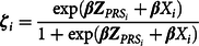 $${{\bf{\zeta }}_i} = {{{{{\exp ({{\beta}}}{{\bf{Z}}_{PR{S_i}}} + {\beta}}{X_i})}} \over {1 + \exp ({\beta}}{{\bf{Z}}_{PR{S_i}}} + {\beta}{X_i})}$$
The result of this estimation process is a single score capturing the observed genetic and environmental risk for a phenotype. The estimation process for calculating GAPS, nonetheless, relies on a series of assumptions that are required to be satisfied. In addition to model assumptions (e.g., linearity, normality and heteroscedasticity; Fox, Reference Fox2016) and the assumptions associated with PRSs, the estimation of the GAPS requires that the level of measurement for the phenotype remains consistent across all estimations. For example, if the PRS was calculated using a dichotomous measure, the estimation of the GAPS should employ the same dichotomous measure. This requirement is a consequence of the differing amount of variation in a phenotype explained by the PRS and environmental constructs across levels of measurement. As such, if the level of measurement for the dependent construct varies between the models, the variation explained by observed genetic and environmental factors could bias the resulting GAPS.
In addition to the statistical control method or GAPS weighting (Guo & Fraser, Reference Guo and Fraser2015), GAPS can be used to match participants to emulate the counterfactual condition created by the MZ twin difference approach. Specifically, respondents with similar observed genetic and observed environmental factors could be matched using the GAPS to mimic the robust counterfactual condition and high internal validity present in a discordant MZ twin model. For instance, respondents with similar GAPS but different educational attainment can be matched, and the resulting matched sample can be used to evaluate the association between educational attainment and future income, which could potentially produce estimates similar to a discordant MZ twin model. Indeed, GAPS can be employed using a variety of matching procedures conventionally used in propensity score matching analyses (see Guo & Fraser, Reference Guo and Fraser2015). For instance, GAPS can be used in conjunction with exact matching (Eq. 7) or caliper matching (Eq. 8; ϵ represents the caliper):
 $${{\zeta }_{(tcomma =comma 1)}} = {\zeta }_{(tcomma =comma 0)}$$
 $$\left\| {{{\bf{\zeta }}_{(t comma =comma 1)}} - {{\bf{\zeta }}_{(t comma =comma 0)}}} \right\| \lt comma \varepsilon $$
Against this backdrop, the current study assessed the validity of the GAPS matching approach by addressing two research questions: (RQ1) What is the degree to which GAPS matching can produce estimates similar to the estimates produced by the MZ twin difference approach? and (RQ2) What is the added value of adjusting for the confounding effects of G × E when estimating the effects of one phenotype on another? To test these research questions, the current study employed simulation analyses to assess how well GAPS matching can approach the estimates produced by the MZ twin difference approach. Nine of 240 simulated comparisons (N = 10,000 for each simulation) will be discussed in the current study to provide a comprehensive comparison between the GAPS matching and discordant MZ twin methods when estimating associations. Footnote 4 The nine simulated examples were selected due to their ability to provide the largest insight into the results across all of the simulated comparisons. Moreover, the selected examples emulate the variance common in complex phenotypes. Specifically, when decomposing the variance in complex phenotypes, a larger portion is attributed to genetic and nonshared environmental factors, while a smaller portion is attributed to the shared environment or unique G × E interactions. That said, all the results for each of the 240 simulations are provided in text files using https://github.com/ianasilver/Genetically-adjusted-propensity-scores-A-comparison-to-discordant-MZ-twin-models, Footnote 5 and an R-script for a randomly specified looped simulation is provided as supplemental materials to permit the estimation and evaluation of GAPS matching across randomly specified phenotypes.
Simulation Analyses: Comparing GAPS Matching to the MZ Difference Approach Footnote 6
Assumptions of Simulation Analyses
The simulation analyses discussed below and the corresponding results compare the GAPS matching approach to the discordant MZ twin approach under the optimal conditions for PRSs. These optimal conditions can be highlighted by discussing the three foundational assumptions of the simulation analyses. First, the simulation analyses assume that PRSs can adjust estimates for the heritability of a phenotype in a manner identical to that of the discordant MZ twin approach. Due to the missing heritability associated with PRSs (Manolio et al., Reference Manolio, Collins, Cox, Goldstein, Hindorff, Hunter, McCarthy, Ramos, Cardon, Chakravarti, Cho, Guttmacher, Kong, Kruglyak, Mardis, Rotimi, Slatkin, Valle, Whittemore and Visscher2009), this assumption would likely not hold when employing the GAPS matching approach in a real data example (illustrated below). Moreover, the effects of the missing heritability on the GAPS matching approach are evaluated and discussed below.
Second, the simulation analyses assume that the discordant MZ twin approach does not adjust for variation associated with the nonshared environment. In a bivariate assessment, this assumption holds true, as the discordance between MZ twins on nonshared environmental conditions will not be adjusted for when estimating the effects of interest (Knopik et al., Reference Knopik, Ndiderhiser, DeFries and Plomin2016). Nevertheless, observable or latent measures of the discordance between MZ twins on nonshared environmental conditions can be introduced into multivariate analyses, adjusting for variation in the nonshared environment. While this assumption might not accurately characterize the extent to which the discordant MZ twin approach can generate robust estimates, the simulation analyses provide a comparison to the baseline discordant MZ twin approach. Supplementary material Appendix C, however, provides a replication of the simulation analyses assuming that observable measures of the discordance between MZ twins on nonshared environmental conditions are introduced into a multivariate analysis. As demonstrated, the results suggest that the discordant MZ twin approach possesses an enhanced ability to estimate the true association when observable or latent measures of the discordance between MZ twins on nonshared environmental conditions are introduced into a multivariate analysis.
Finally, due to the difficulties associated with comparing two techniques reliant on different data structures, the simulation analyses assume that the matching error rate will be identical when conducting GAPS matching and difference score analyses using MZ twins. This assumption primarily exists due to the inability to simulate a single dataset that can be representative of both singletons and MZ twin pairs, as well as the difficulties associated with ensuring that the effects and error structures are identical across multiple datasets with different simulation specifications (Knopik et al., Reference Knopik, Ndiderhiser, DeFries and Plomin2016). The matching error rate of the simulation analyses equally influenced the slope coefficients produced by the MZ difference score evaluation and the GAPS matching approach, which is a limitation of the simulation as MZ twin pairs inherently possess a low matching error rate (i.e., the rate of misidentifying MZ twin pairs; Knopik et al., Reference Knopik, Ndiderhiser, DeFries and Plomin2016). Nevertheless, Supplementary Appendix F is provided to demonstrate that the matching procedure itself has limited effects on the observed difference between the discordant MZ twin approach and the GAPS matching approach.
Specification of the Dichotomous Independent Variable (X)
To assess the validity of the GAPS matching approach, 240 unique conditions were simulated to emulate potential phenotypic variation in an independent variable of interest. As demonstrated in Figure 1, the variation in the dichotomous independent variable (
X
) was specified to be equal to a predetermined proportion (p) of the genetic (A), shared environment (C), nonshared environment (E) and residual variation (e; see mathematical equations in Supplementary Appendix A and available R-scripts).
Footnote 7
Across 240 simulations, three methods were employed to differ the amount of variation contributed to
X
by A, C and E. First, variation in
X
was equal to .05 incremental increases — from 0 to .95 — in A, while the amount of variation in
X
contributed by C and E were equal. The independent variable (
X
) was dichotomized to permit a more intuitive analytical strategy for comparing the GAPS matching approach to the discordant MZ twin approach. To ensure that the estimated scores did not perfectly predict
X
, the amount of residual variation (rv) in
X
always equaled .04. For example, the first specification was
 ${\bf{X}} = { .000_{\bf{A}}} + { .480_{\bf{E}}}comma + { .480_{\bf{C}}} + { .040_{{\bf{rv}}}}$
, the midpoint of the distribution of incremental specifications was
${\bf{X}} = { .000_{\bf{A}}} + { .480_{\bf{E}}}comma + { .480_{\bf{C}}} + { .040_{{\bf{rv}}}}$
, the midpoint of the distribution of incremental specifications was
 ${\bf{X}} = { .450_{\bf{A}}} \ + { .255_{\bf{E}}} + { .255_{\bf{C}}} + { .040_{{\bf{rv}}}}$
and the final specification was
${\bf{X}} = { .450_{\bf{A}}} \ + { .255_{\bf{E}}} + { .255_{\bf{C}}} + { .040_{{\bf{rv}}}}$
and the final specification was
 ${\bf{X}} = { .950_{\bf{A}}} + { .005_{\bf{E}}} + { .005_{\bf{C}}} + { .040_{{\bf{rv}}}}$
(Figure 2).
${\bf{X}} = { .950_{\bf{A}}} + { .005_{\bf{E}}} + { .005_{\bf{C}}} + { .040_{{\bf{rv}}}}$
(Figure 2).
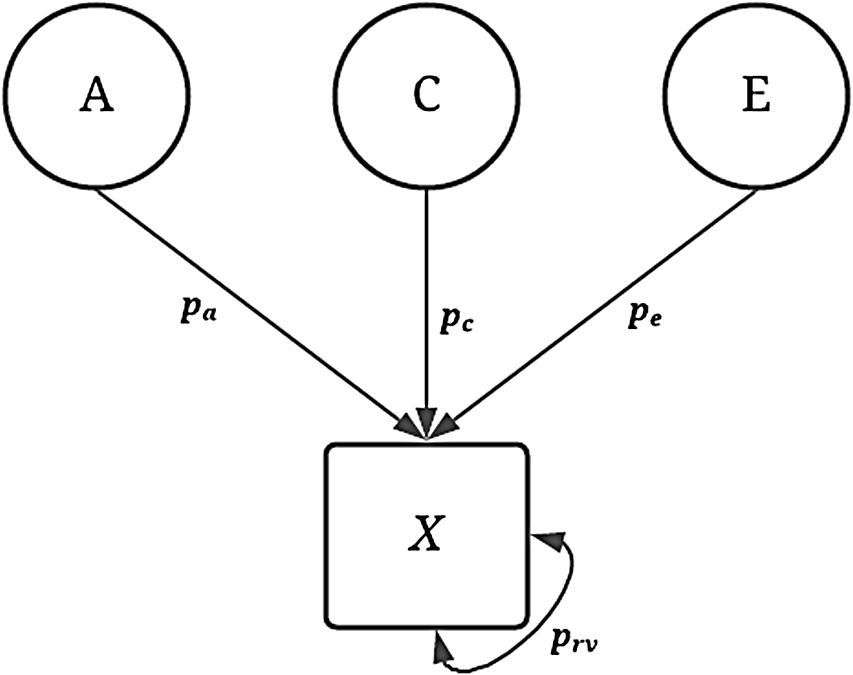
Fig. 1. Visual depiction of specified variation in the simulated treatment variable ( X ) without interactions.
Note: A represents the genetic effect, pa represents the proportion of variation in X predicted by A, C represents the shared environment, pc represents the proportion of variation in X predicted by C, E represents the nonshared environment, pe represents the proportion of variation in X predicted by E, X represents a dichotomous treatment construct. The double-headed arrow represents the residual variation in the specification of X, where prv represents the proportion of residual variation.
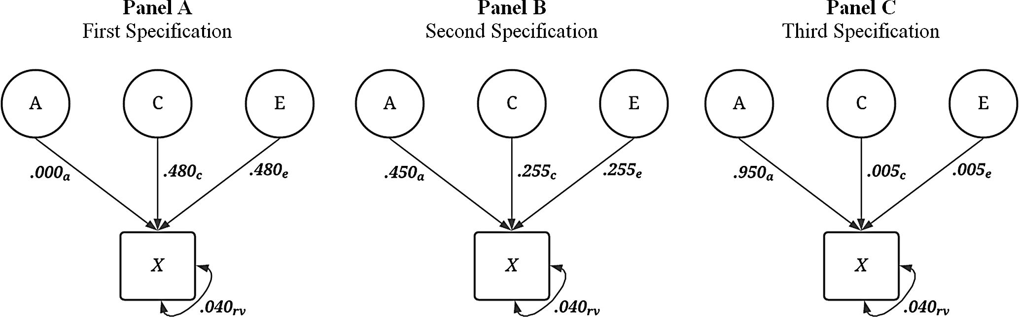
Fig. 2. Visual depiction of specified variation in the simulated treatment variable ( X ) without interactions
Second, the variation in
X
followed the same procedure above (i.e., .05 incremental increases from 0 to .95 for A), but the variation in
X
contributed by C was three times that contributed by E. For example, the first specification was
 ${\bf{X}} = { .000_{\bf{A}}} + { .240_{\bf{E}}} + { .720_{\bf{C}}} + { .040_{{\bf{rv}}}}$
, the middle of the distribution of incremental specifications was
${\bf{X}} = { .000_{\bf{A}}} + { .240_{\bf{E}}} + { .720_{\bf{C}}} + { .040_{{\bf{rv}}}}$
, the middle of the distribution of incremental specifications was
 ${\bf{X}} = { .450_{\bf{A}}} + { .1275_{\bf{E}}} + { .3825_{\bf{C}}} + { .040_{{\bf{rv}}}}$
and the final specification was
${\bf{X}} = { .450_{\bf{A}}} + { .1275_{\bf{E}}} + { .3825_{\bf{C}}} + { .040_{{\bf{rv}}}}$
and the final specification was
 ${\bf{X}} = { .950_{\bf{A}}} + { .0025_{\bf{E}}} + { .0075_{\bf{C}}} + { .040_{{\bf{rv}}}}$
. The third condition of variation in
X
maintained the same incremental increases in A as the prior conditions, whereas the variation in
X
contributed by E was three times that contributed by C (i.e., the reverse of the second condition). For example, the first specification was
${\bf{X}} = { .950_{\bf{A}}} + { .0025_{\bf{E}}} + { .0075_{\bf{C}}} + { .040_{{\bf{rv}}}}$
. The third condition of variation in
X
maintained the same incremental increases in A as the prior conditions, whereas the variation in
X
contributed by E was three times that contributed by C (i.e., the reverse of the second condition). For example, the first specification was
 ${\bf{X}} = { .000_{\bf{A}}} + { .720_{\bf{E}}} + { .240_{\bf{C}}} + { .040_{{\bf{rv}}}}$
, the middle of the distribution of incremental specifications was
${\bf{X}} = { .000_{\bf{A}}} + { .720_{\bf{E}}} + { .240_{\bf{C}}} + { .040_{{\bf{rv}}}}$
, the middle of the distribution of incremental specifications was
 ${\bf{X}} = { .450_{\bf{A}}} + { .3825_{\bf{E}}} + { .1275_{\bf{C}}} + { .040_{{\bf{rv}}}}$
and the final specification was
${\bf{X}} = { .450_{\bf{A}}} + { .3825_{\bf{E}}} + { .1275_{\bf{C}}} + { .040_{{\bf{rv}}}}$
and the final specification was
 ${\bf{X}} = { .950_{\bf{A}}} + { .0075_{\bf{E}}} + { .0025_{\bf{C}}} + { .040_{{\bf{rv}}}}$
.
${\bf{X}} = { .950_{\bf{A}}} + { .0075_{\bf{E}}} + { .0025_{\bf{C}}} + { .040_{{\bf{rv}}}}$
.
Subsequently, a series of specifications for
X
included a G × E between A and C, A and E, or both. The specifications are illustrated in Figure 3. For each of the specifications including a G × E, 20% of the amount of variation contributed by each component was redirected to the interaction specification (Figure 3). For example, using Panel A of Figure 3, the first specification was
 ${\bf{X}} = { .000_{\bf{A}}} + { .384_{\bf{E}}} + { .480_{\bf{C}}} + { .0960_{{\bf{(A*E)}}}} + { .040_{{\bf{rv}}}}$
, the middle of the distribution of incremental specifications was
${\bf{X}} = { .000_{\bf{A}}} + { .384_{\bf{E}}} + { .480_{\bf{C}}} + { .0960_{{\bf{(A*E)}}}} + { .040_{{\bf{rv}}}}$
, the middle of the distribution of incremental specifications was
 ${\bf{X}} = { .360_{\bf{A}}} + { .204_{\bf{E}}} + { .255_{\bf{C}}} + { .141_{{\bf{(A*E)}}}} + { .040_{{\bf{rv}}}}$
and the final specification was
${\bf{X}} = { .360_{\bf{A}}} + { .204_{\bf{E}}} + { .255_{\bf{C}}} + { .141_{{\bf{(A*E)}}}} + { .040_{{\bf{rv}}}}$
and the final specification was
 ${\bf{X}} = { .760_{\bf{A}}} + { .004_{\bf{E}}} + { .005_{\bf{C}}} + { .191_{{\bf{(A*E)}}}} + { .040_{{\bf{rv}}}}$
. Using Panel C of Figure 3, the first specification was
${\bf{X}} = { .760_{\bf{A}}} + { .004_{\bf{E}}} + { .005_{\bf{C}}} + { .191_{{\bf{(A*E)}}}} + { .040_{{\bf{rv}}}}$
. Using Panel C of Figure 3, the first specification was
 ${\bf{X}} = { .000_{\bf{A}}} + { .384_{\bf{E}}} + { .384_{\bf{C}}} + { .096_{{\bf{(A*E)}}}} + { .096_{{\bf{(A*C)}}}} + { .040_{{\bf{rv}}}}$
, the middle of the distribution of incremental specifications was
${\bf{X}} = { .000_{\bf{A}}} + { .384_{\bf{E}}} + { .384_{\bf{C}}} + { .096_{{\bf{(A*E)}}}} + { .096_{{\bf{(A*C)}}}} + { .040_{{\bf{rv}}}}$
, the middle of the distribution of incremental specifications was
 ${\bf{X}} = { .270_{\bf{A}}} + { .204_{\bf{E}}} + { .204_{\bf{C}}} + { .141_{{\bf{(A*E)}}}} + { .141_{{\bf{(A*C)}}}} + { .040_{{\bf{rv}}}}$
and the final specification was
${\bf{X}} = { .270_{\bf{A}}} + { .204_{\bf{E}}} + { .204_{\bf{C}}} + { .141_{{\bf{(A*E)}}}} + { .141_{{\bf{(A*C)}}}} + { .040_{{\bf{rv}}}}$
and the final specification was
 ${\bf{X}} = { .570_{\bf{A}}} + { .004_{\bf{E}}} + { .004_{\bf{C}}} + { .191_{{\bf{(A*E)}}}} + { .191_{{\bf{(a*c)}}}} + { .040_{{\bf{rv}}}}$
. Following these examples, 240 specifications of
X
were created wherein 60 specifications only included direct effects and 180 specifications included direct and interactive effects. The dichotomous indicator of
X
was then used to specify the variation in
Y.
${\bf{X}} = { .570_{\bf{A}}} + { .004_{\bf{E}}} + { .004_{\bf{C}}} + { .191_{{\bf{(A*E)}}}} + { .191_{{\bf{(a*c)}}}} + { .040_{{\bf{rv}}}}$
. Following these examples, 240 specifications of
X
were created wherein 60 specifications only included direct effects and 180 specifications included direct and interactive effects. The dichotomous indicator of
X
was then used to specify the variation in
Y.
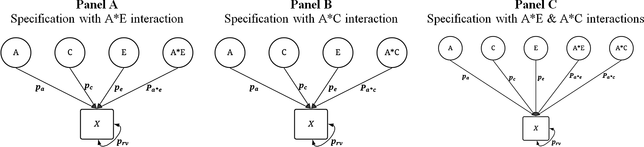
Fig. 3. Visual depiction of specified variation in the simulated treatment variable ( X ) with interactions
Specification of the Dependent Variable (Y)
The simulations were specified in a manner to provide a complete comparison between the estimates produced using GAPS matching to the estimates produced from a discordant MZ twin model. The dependent variable ( Y ) was consistently specified across all the noninteractive conditions of the dichotomous independent variable ( X ). As illustrated by Figure 4, variation in Y was specified to be the product of the association (i.e., the slope coefficient) between X and Y (b = 1.00), as well as A (representing the genetic effects), C (representing the shared environment), E (representing the nonshared environment) and residual variation. The influence of A, C and E on Y was specified as 1.25 to ensure that a substantive amount of variation in Y was predicted by A, C and E. The specification above generates a substantial amount of confounding in the analytical model and assumes that only a limited amount of error in Y exists after accounting for the genetic, shared environment and nonshared environment effects. Footnote 8
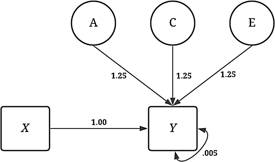
Fig. 4. Visual depiction of specified variation in the simulated independent variable ( Y ) without interactions
In addition to the conditions illustrated above, three specifications of the dependent variable with interaction terms were created (see Figure 5) corresponding to the specifications of X that included the respective interaction. First, an interaction between A and E was specified to predict variation in Y . Second, an interaction between A and C was specified to predict variation in Y . Finally, interactions between A and E as well as A and C were specified to predict variation in Y . Overall, the specifications of the IV and DV provide for a comparison between the GAPS matching and MZ difference score approaches in three conditions: (1) in the absence of interactions, (2) in the presence of a gene-shared environment interaction and (3) in the presence of gene-nonshared environment interactions.
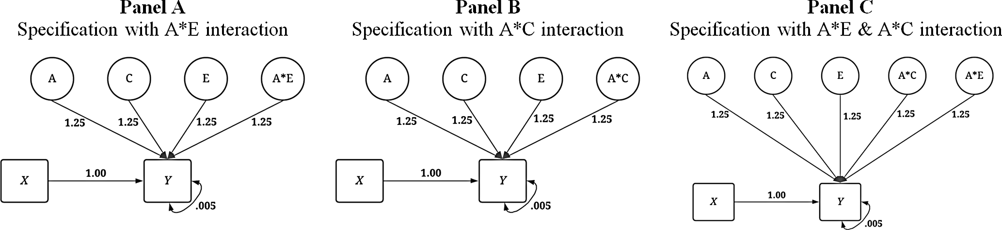
Fig. 5. Visual depiction of specified variation in the simulated independent variable ( Y ) with interactions
Comparing Discordant MZ twin Approach to GAPS Matching Approach
Although various modeling strategies can be used to compare the discordant MZ twin approach to the GAPS matching approach, the most intuitive procedure is postmatching comparisons. Figure 6 provides visual depictions of the analytical approach. The matching was conducted by regressing X on all or a proportion of the variation in A, C and E using a binary logistic regression model. The results of the model were then used to calculate a predicted probability — creating a GAPS or a score approximating an MZ difference approach — which determined how cases that experienced the condition ( X = 1) were matched to cases that did not experience the condition ( X = 0). When approximating an MZ difference approach, the binary logistic regression model regressed X on all the variation in A and C to emulate the ability to adjust for all of the genetic and shared environmental factors cofounding an association of interest. When estimating the GAPS, X was regressed on all of the variation in A and a portion of the variation in C and E to emulate the postulated ability to adjust for all of the genetic factors and some of the shared environmental and nonshared environmental factors cofounding an association of interest. Importantly, although the GAPS and score approximating an MZ difference approach were calculated identically, it was assumed that the predicted probability created using all of the variation in A and C would best emulate the MZ difference approach.
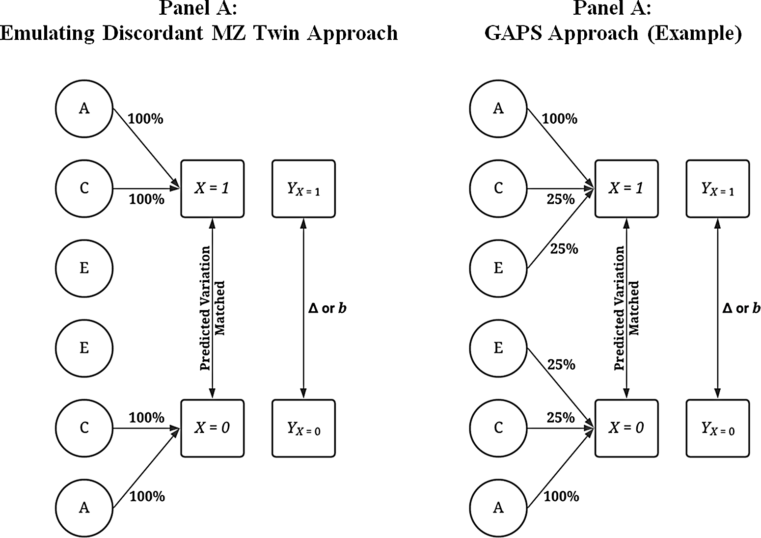
Fig. 6. Visual examples of the analytical matching approach.
Note: Percentage values represent the amount of variation in X predicted by A, C and E used to predict values on X . For example, .25 of E when E predicted 38.2% of the variation in X indicates that 9.56% of the variation of X (contributed by the nonshared environment) is adjusted for in the matching process. A represents the genetic effect, C represents the shared environment, E represents the nonshared environment and X represents a dichotomous independent variable. Y represents the dependent variable, and Δ or b represents the difference in the outcomes between the treatment ( X = 1) and control cases ( X = 0). The matching procedure described does not fully emulate the discordant MZ twin approach as identical twins would share the same genetic materials. A predicted probability was calculated using a logistic regression with all of or subcomponents of A (x1-x4), C (x5-x8) or E (x9-x12; see Appendix A and R-scripts) serving as the independent variables and X serving as the dependent variable. The resulting predicted probability was then used to match participants.
Simulated cases that scored a 0 on X were matched to simulated cases that scored a 1 on
X
using nearest neighbor matching (caliper = .05) at varying amounts of A, C and E predicting scores on
X
. To emulate the discordant MZ twin approach (Panel A of Figure 6), the amount of information that simulated cases were matched on equaled all of the variation in
X
that can be attributed to genetic and shared environmental factors. For instance, if the specification of
 ${\bf{X}} = { .450_{\bf{A}}} + { .1275_{\bf{E}}} + { .3825_{\bf{C}}} + { .040_{{\bf{rv}}}}$
, the MZ matching procedure used all the variation in
X
contributed by A (.45) and by C (.3825) to match the participants.
${\bf{X}} = { .450_{\bf{A}}} + { .1275_{\bf{E}}} + { .3825_{\bf{C}}} + { .040_{{\bf{rv}}}}$
, the MZ matching procedure used all the variation in
X
contributed by A (.45) and by C (.3825) to match the participants.
While the approach outlined above emulates the discordant MZ twin approach, it is not exact because identical twins would share identical genetic material. The matching technique employed — nearest neighbor matching with a caliper of .05 — only produces pairs with very similar scores on A rather than pairs with identical scores on A (Guo & Fraser, Reference Guo and Fraser2015). However, given that both the MZ twin approach and the GAPS matching approach employed the same seed and a caliper of .05, the differences observed in the slope coefficients using a caliper = .01, .001 or exact matching when comparing the MZ twin approach to the GAPS matching approach were extremely similar to the differences observed when nearest neighbor matching with a caliper of .05 was employed. Nearest neighbor matching was favored in the current simulation due to the substantial amount of time added to the simulation analysis when exact matching was employed, as well as concerns related to the sample size for the postmatching analyses emulating the discordant MZ twin approach. Two R-scripts used to conduct the analyses, however, are provided for replication and alteration purposes. After matching the participants, a linear regression model was estimated, where Y was regressed on X for only the matched subsample (where A and C were held constant across values of X ). The resulting estimate, similar to a discordant MZ twin model, therefore adjusted for the confounding influence of A and C, since shared genetic factors and shared environmental factors were both held constant within the matched subsample.
A similar matching procedure was also employed and cases were matched on their associated GAPS score, rather than on A and C (Panel B of Figure 6). This matching procedure assumed that the all genetic confounding between
X
and
Y
would be captured by the PRS used to create the GAPS score.
Footnote 9
In addition to matching participants on all the genetic confounding between
X
and
Y
, the simulated cases were matched to each other using fluctuating amounts of variation contributed to
X
by C and E. For example, if the specification of
 ${\bf{X}} = { .450_{\bf{A}}} + { .1275_{\bf{E}}} + { .3825_{\bf{C}}} + { .040_{{\bf{rv}}}}$
, one matching procedure would use all the variation contributed by A (.45), 25% of the variation contributed by C (.096) and 25% of the variation from E (.032) to match the simulated cases (Panel B of Figure 6).
${\bf{X}} = { .450_{\bf{A}}} + { .1275_{\bf{E}}} + { .3825_{\bf{C}}} + { .040_{{\bf{rv}}}}$
, one matching procedure would use all the variation contributed by A (.45), 25% of the variation contributed by C (.096) and 25% of the variation from E (.032) to match the simulated cases (Panel B of Figure 6).
Furthermore, interactions between A and E, and/or A and C were included in the matching procedures when the respective specifications of X and Y were the focus of the postmatching analysis. In total, for each specification of X approximately 20 matching procedures were completed, which was designed to provide a comprehensive illustration of how much variation in X needs to be captured by GAPS to produce estimates similar to estimates produced by the discordant MZ twin approach. All simulated comparisons were completed using the Ohio Supercomputer (Ohio Supercomputer Center, 1987). Below, we highlight specifications of X and the respective association between X and Y , to illustrate the information needed for GAPS matching to produce slope coefficients that approach the estimates produced by the discordant MZ twin approach in nine distinct circumstances.
Example 1: No Interactions
Example 1 illustrates the conditions needed for postmatching GAPS slope coefficients to be close to or improve upon the slope coefficients produced by discordant MZ twin methods. In this example, the specification of the variation in
X
was set based on a twin-based meta-analysis of common complex traits (Polderman et al., Reference Polderman, Benyamin, De Leeuw, Sullivan, Van Bochoven, Visscher and Posthuma2015). Specifically, corresponding with complex traits, 45% of the variation in
X
was attributed to genetic effects, 38.25% of the variation in
X
was attributed to the nonshared environment and 12.75% of the variation in
X
was attributed to the shared environment. Therefore, the formula to specify
X
was
 ${\bf{X}} = { .450_{\bf{A}}} + { .3825_{\bf{E}}} + { .1275_{\bf{C}}} + { .040_{{\bf{rv}}}}$
. The dependent variable (
Y
) was specified following the depiction in Figure 4. Succeeding the matching procedure, the association between
Y
and
X
was estimated using the matched subsamples and an Ordinary Least Squares (OLS) regression model. The derived estimates and 95% confidence intervals for each postmatching subsample were then plotted to allow for comparison between the MZ and GAPS matching procedures.
${\bf{X}} = { .450_{\bf{A}}} + { .3825_{\bf{E}}} + { .1275_{\bf{C}}} + { .040_{{\bf{rv}}}}$
. The dependent variable (
Y
) was specified following the depiction in Figure 4. Succeeding the matching procedure, the association between
Y
and
X
was estimated using the matched subsamples and an Ordinary Least Squares (OLS) regression model. The derived estimates and 95% confidence intervals for each postmatching subsample were then plotted to allow for comparison between the MZ and GAPS matching procedures.
Results
Figure 7 provides the estimates and 95% confidence intervals for the association between X and Y derived from the matched subsamples. As a reminder, the specified slope coefficient for the association is 1.00 and is represented by the solid vertical line in the figure. The specifications on the y-axis provide the proportion of the variation in X attributed to the specified component used to match participants. For example, 1 * A indicates that all the genetic variation in X (.45) was used to match the participants, and .25 * E indicates that 25% of the variation in X attributed to the nonshared environment (E; .3825(.25) = .0955) was used to match the participants. The estimate at the top of Figure 7 (1 * A; 1 * C) provides an approximation for the estimate produced by a discordant MZ twin model. The estimates derived from the matched subsamples, using the indicated matching specifications, in between the upper and lower dashed lines were further from the specified slope coefficient (1.00) than the estimate derived from the approximated MZ twin subsample (b = 1.253). The estimates derived from the matched subsamples below the lower dashed line were equal distance or closer to the specified slope coefficient (1.00) than the estimate derived from the approximated MZ twin subsample (b = 1.253). Overall, the results suggest that the MZ difference score approached the specified slope coefficient (1.00) more closely than GAPS matching when less environmental information (E and C) is used to create the GAPS. Nevertheless, GAPS matching generally approached the specified slope coefficient (1.00) more closely than discordant MZ twin models when more environmental information (>50% of the variation in E and C) is used to create the GAPS. Overall, the GAPS matching slope coefficient remained substantively different from the specified slope coefficient (1.00) on average (b ≈ 1.25) across the estimated comparisons. Importantly, these estimates assumed that the polygenic score would capture all the genetic variation in X (.45).
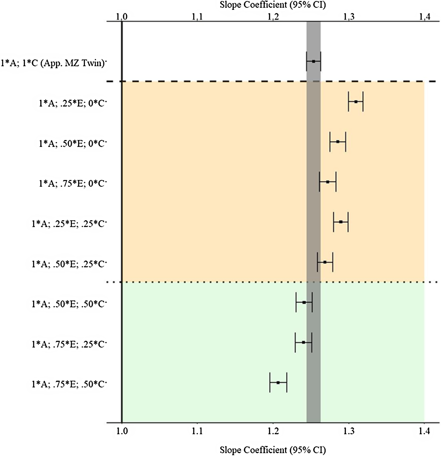
Fig. 7. (Example 1). Slope coefficients of Y regressed on X differentially adjusting for the confounding influence of genetic, shared environmental and nonshared environmental effects.
Note: A = genetics, E = nonshared environment, C = shared environment. The true association between Y and X is 1.00 (Starting N = 10,000). For the current example, variation in X was specified as 45 % genetic, 38.2% nonshared environment, 12.8% shared environment and 4% error. Genetic, shared environmental and nonshared environmental factors equally contributed to the variation in Y . All estimates were derived from a postmatching OLS model. Matching was completed using nearest neighbor matching with a caliper of .05. The orange area provides the specifications that performed further away from the true point estimate (1.00) than the approximation of discordant MZ twin methods, and the green area provides the specifications that were closer to the true point estimate (1.00) than the approximation of discordant MZ twin methods. The proportions on the y-axis represent the proportion of the variation in X contributed by the specified component (A, C or E) that is adjusted for by the model. For example, .25 * E indicates that 9.56% of the variation of X (contributed by the nonshared environment) is adjusted for in the model.
Examining the effects of missing heritability
To illustrate the effects of missing heritability on estimates derived from GAPS matching, nine additional matching subsamples were created. The specified proportion of the variation in X attributed to the genetic and environmental components were used to match simulated cases. The results overwhelmingly demonstrated that estimates produced by GAPS matching were further from the specified slope coefficient (1.00) than the discordant MZ twin estimate. This finding suggests that the missing heritability could substantively diminish the ability of GAPS matching to produce estimates equal to the estimates produced by discordant MZ twin methods. Generally, we recognize that GAPS matching will not perfectly emulate the discordant MZ twin approach, because it is unlikely that PRSs will predict the same amount of genetic variation as the discordant MZ twin approach (Table 1; Slatkin, Reference Slatkin2009). However, we expect the performance of GAPS matching will be enhanced as larger GWAS are conducted and PRSs are improved.
Table 1. Demonstration of the effects of missing heritability on Example 1 (simulation starting N = 10,000)
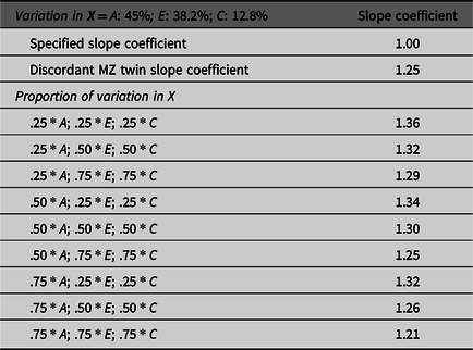
Note: A = genetics, E = nonshared environment, C = shared environment. For the current example, variation in X was specified as 45 % genetic, 38.2% nonshared environment, 12.8% shared environment and 4% error. Genetic, shared environmental and nonshared environmental factors equally contributed to the variation in Y . All estimates were derived from a postmatching OLS model. Matching was completed using nearest neighbor matching with a caliper of .05. The proportions represent the proportion of the variation in X contributed by the specified component (A, C or E) that is adjusted for by the model. For example, .25 * E indicates that 9.56% of the variation of X (contributed by the nonshared environment) is adjusted for in the model.
Results from low and high genetic contribution comparisons
To provide additional comparisons between the GAPS matching approach and discordant MZ twin methods, simulations with low (
 ${\bf{X}} = { .100_{\bf{A}}} + { .645_{\bf{E}}} + { .215_{\bf{C}}} + { .040_{{\bf{rv}}}}$
) and high (
${\bf{X}} = { .100_{\bf{A}}} + { .645_{\bf{E}}} + { .215_{\bf{C}}} + { .040_{{\bf{rv}}}}$
) and high (
 ${\bf{X}} = { .800_{\bf{A}}} + { .120_{\bf{E}}} + { .040_{\bf{C}}} + { .040_{{\bf{rv}}}}$
) genetic contribution to
X
were plotted in Figure 8. As demonstrated, the pattern of findings associated with the low and high genetic contribution to
X
was similar to the pattern of findings in Figure 7.
${\bf{X}} = { .800_{\bf{A}}} + { .120_{\bf{E}}} + { .040_{\bf{C}}} + { .040_{{\bf{rv}}}}$
) genetic contribution to
X
were plotted in Figure 8. As demonstrated, the pattern of findings associated with the low and high genetic contribution to
X
was similar to the pattern of findings in Figure 7.
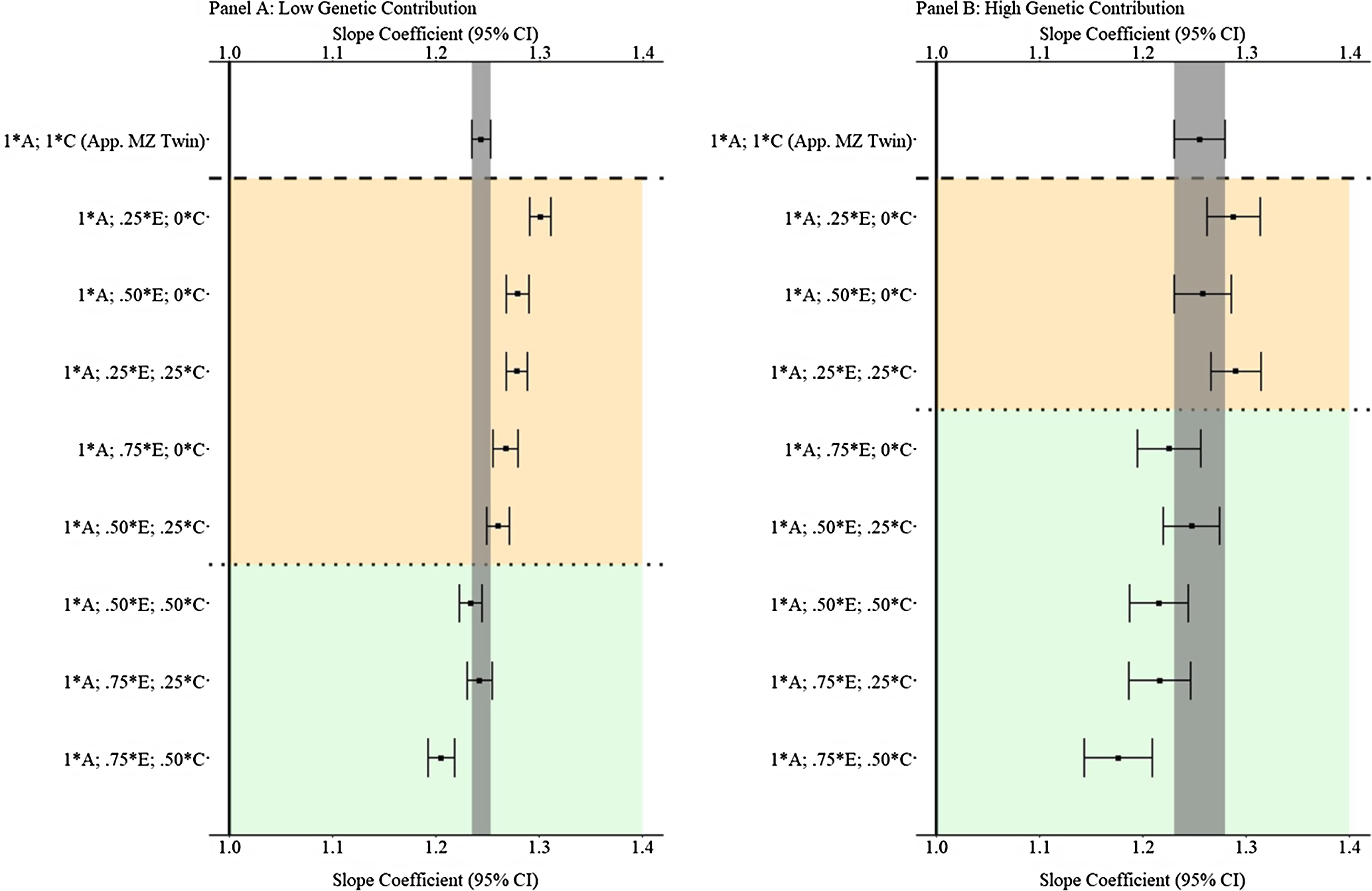
Fig. 8. (Example 1). Slope coefficients of Y regressed on X with low and high genetic contribution to the variation in X .
Note: A = genetics, E = nonshared environment, C = shared environment. The true association between Y and X is 1.00 (Starting N = 10,000). For the current example, low genetic contribution: 10 % genetic, 64.5% nonshared environment, 21.5% shared environment and 4% error. High genetic contribution: 80 % genetic, 12% nonshared environment, 4% shared environment and 4% error. Genetic, shared environmental and nonshared environmental factors equally contributed to the variation in Y . All estimates were derived from a postmatching OLS model. Matching was completed using nearest neighbor matching with a caliper of .05. The orange area provides the specifications that performed further away from the true point estimate (1.00) than the approximation of discordant MZ twin methods, and the green area provides the specifications that were closer to the true point estimate (1.00) than the approximation of discordant MZ twin methods. The proportions on the y-axis represent the proportion of the variation in X contributed by the specified component (A, C or E) that is adjusted for by the model.
Example 2: Interaction Between a and E
Example 2 builds upon the condition presented in Example 1 through the inclusion of a GxE between the genetic effects and the nonshared environment. Distinct from the discordant MZ twin approach, GAPS matching provides the ability to adjust estimates for the confounding effects of genetic-nonshared environment interactions. As such, Example 2 is intended to evaluate if, and how well, the ability to obtain the specified slope coefficient (1.00) is enhanced through the inclusion of a G × E in a GAPS compared to the discordant MZ twin approach. In Example 2, a proportion (∼20%) of the variation in
X
initially attributed to genetic factors and the nonshared environment was reclassified to be attributed to an interaction between genetic factors and the nonshared environment. As such, the variation in
X
was specified as
 ${\bf{X}} = { .360_{\bf{A}}} + { .306_{\bf{E}}} + { .128_{\bf{C}}} + { .167_{({\bf{A}}*{\bf{E}})}} + { .040_{{\bf{rv}}}}$
. Additionally, the independent variable (
Y
) for the current example was specified following Figure 5.
${\bf{X}} = { .360_{\bf{A}}} + { .306_{\bf{E}}} + { .128_{\bf{C}}} + { .167_{({\bf{A}}*{\bf{E}})}} + { .040_{{\bf{rv}}}}$
. Additionally, the independent variable (
Y
) for the current example was specified following Figure 5.
Results
Figure 9 provides the estimated slope coefficients of the association between X and Y , derived from the various matching procedures, for the A * E specification. As demonstrated, the confounding influence of the G × E generates estimates further from the true association (1.00) than the estimates observed in Example 1. Furthermore, distinct from Example 1, only four estimates using the GAPS matching approach were more biased than the estimates derived from the MZ twin approach (b = 1.405). The slope coefficients from the discordant MZ twin approach were likely more biased than the majority of the GAPS matching estimates as a result of the inability to capture any variation associated with the nonshared environment or the G × E. Moreover, accounting for the knowledge that missing heritability likely upwardly biases the estimates derived from GAPS matching, the findings suggest GAPS matching can produce estimates close to discordant MZ twin methods if a genetic nonshared environment interaction (G × E) confounds the association between X and Y .
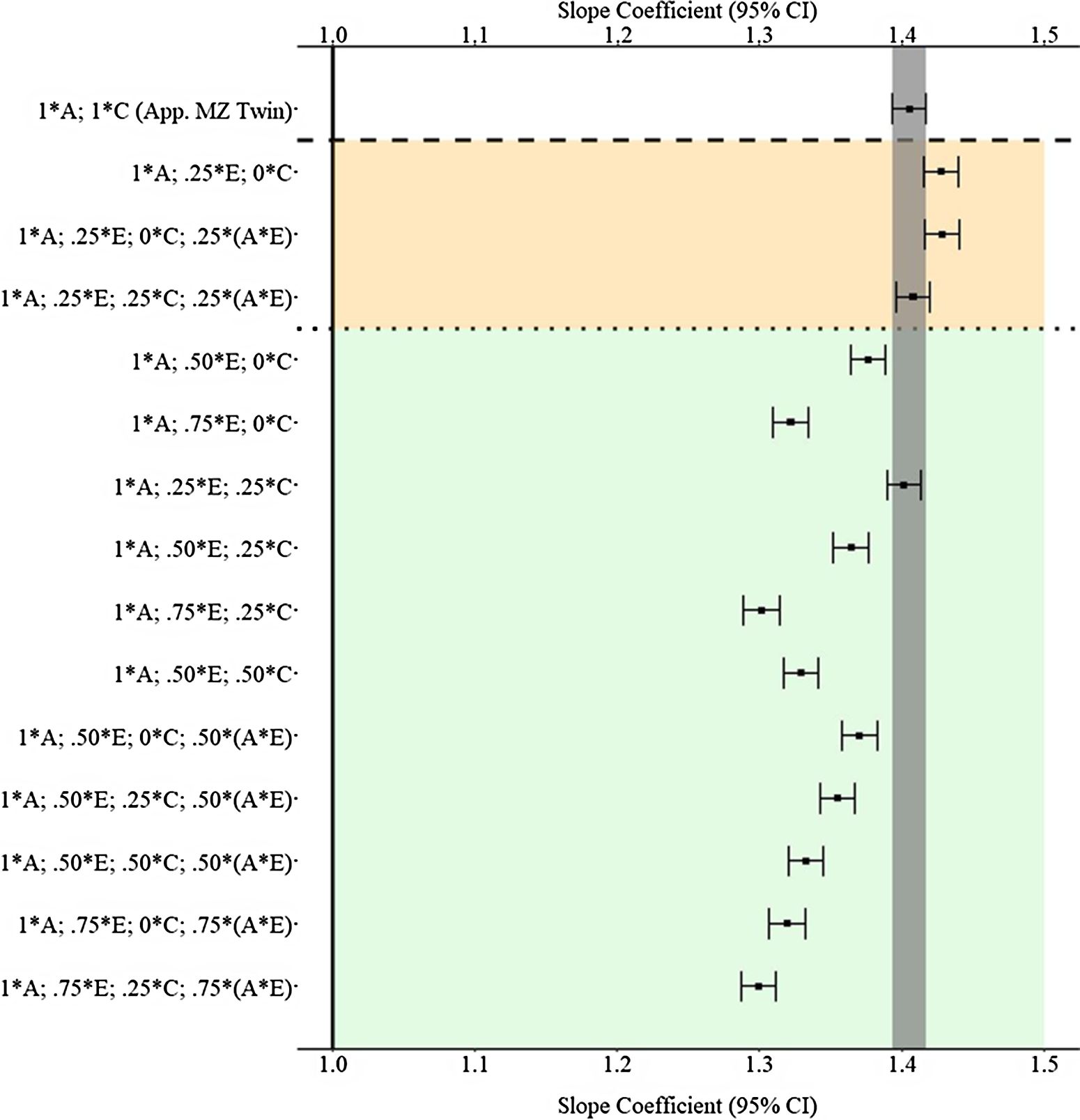
Fig. 9. (Example 2). Slope coefficients of Y regressed on X differentially adjusting for the confounding influence of genetic, shared environmental and nonshared environmental effects.
Note: A = genetics, E = nonshared environment, C = shared environment. The true association between Y and X is 1.00 (Starting N = 10,000). For the current example, variation in X was specified as 36 % genetic, 30.6% nonshared environment, 12.8% shared environment, 16.7% genetic* nonshared environment and 4% error. Genetic, shared environmental and nonshared environmental factors equally contributed to the variation in Y. All estimates were derived from a postmatching OLS model. Matching was completed using nearest neighbor matching with a caliper of .05. The orange area provides the specifications that performed further away from the true point estimate (1.00) than the approximation of discordant MZ twin methods, and the green area provides the specifications that were closer to the true point estimate (1.00) than the approximation of discordant MZ twin methods. The proportions on the y-axis represent the proportion of the variation in X contributed by the specified component (A, C or E) that is adjusted for by the model. For example, .25 * E indicates that 7.7% of the variation of X (attributed to the nonshared environment) is adjusted for in the model.
Results from low and high genetic contribution comparisons
Like Example 1, comparisons with low (
 $${\bf{X}} = { .} 080_{\bf{A}} + { .516_{\bf{E}}} + { .215_{\bf{C}}} + { .149_{({\bf{A}}*{\bf{E}})}} + { .040_{{\bf{rv}}}}$
) and high (
$${\bf{X}} = { .} 080_{\bf{A}} + { .516_{\bf{E}}} + { .215_{\bf{C}}} + { .149_{({\bf{A}}*{\bf{E}})}} + { .040_{{\bf{rv}}}}$
) and high (
 ${\bf{X}} = { .640_{\bf{A}}} + { .096_{\bf{E}}} + { .040_{\bf{C}}} + { .184_{({\bf{A}}*{\bf{E}})}} + { .040_{{\bf{rv}}}}$
) genetic contribution to
X
were also plotted. The findings presented in Figure 10 illustrated that GAPS matching can generally produce slope coefficients that are equivalent or closer to the specified slope coefficient than the discordant MZ twin approach when a G × E confounds the association between
X
and
Y
. At the extreme, Panel B in Figure 10 illustrates that at high genetic contribution to
X
, GAPS matching can produce estimates similar to or outperform the estimates from the discordant MZ twin approach when any combination of genetic and nonshared environmental information is used to create GAPS. This finding suggests that the ability to adjust estimates for G × E interactions in GAPS matching could be a substantive advancement when compared to the discordant MZ twin approach.
${\bf{X}} = { .640_{\bf{A}}} + { .096_{\bf{E}}} + { .040_{\bf{C}}} + { .184_{({\bf{A}}*{\bf{E}})}} + { .040_{{\bf{rv}}}}$
) genetic contribution to
X
were also plotted. The findings presented in Figure 10 illustrated that GAPS matching can generally produce slope coefficients that are equivalent or closer to the specified slope coefficient than the discordant MZ twin approach when a G × E confounds the association between
X
and
Y
. At the extreme, Panel B in Figure 10 illustrates that at high genetic contribution to
X
, GAPS matching can produce estimates similar to or outperform the estimates from the discordant MZ twin approach when any combination of genetic and nonshared environmental information is used to create GAPS. This finding suggests that the ability to adjust estimates for G × E interactions in GAPS matching could be a substantive advancement when compared to the discordant MZ twin approach.
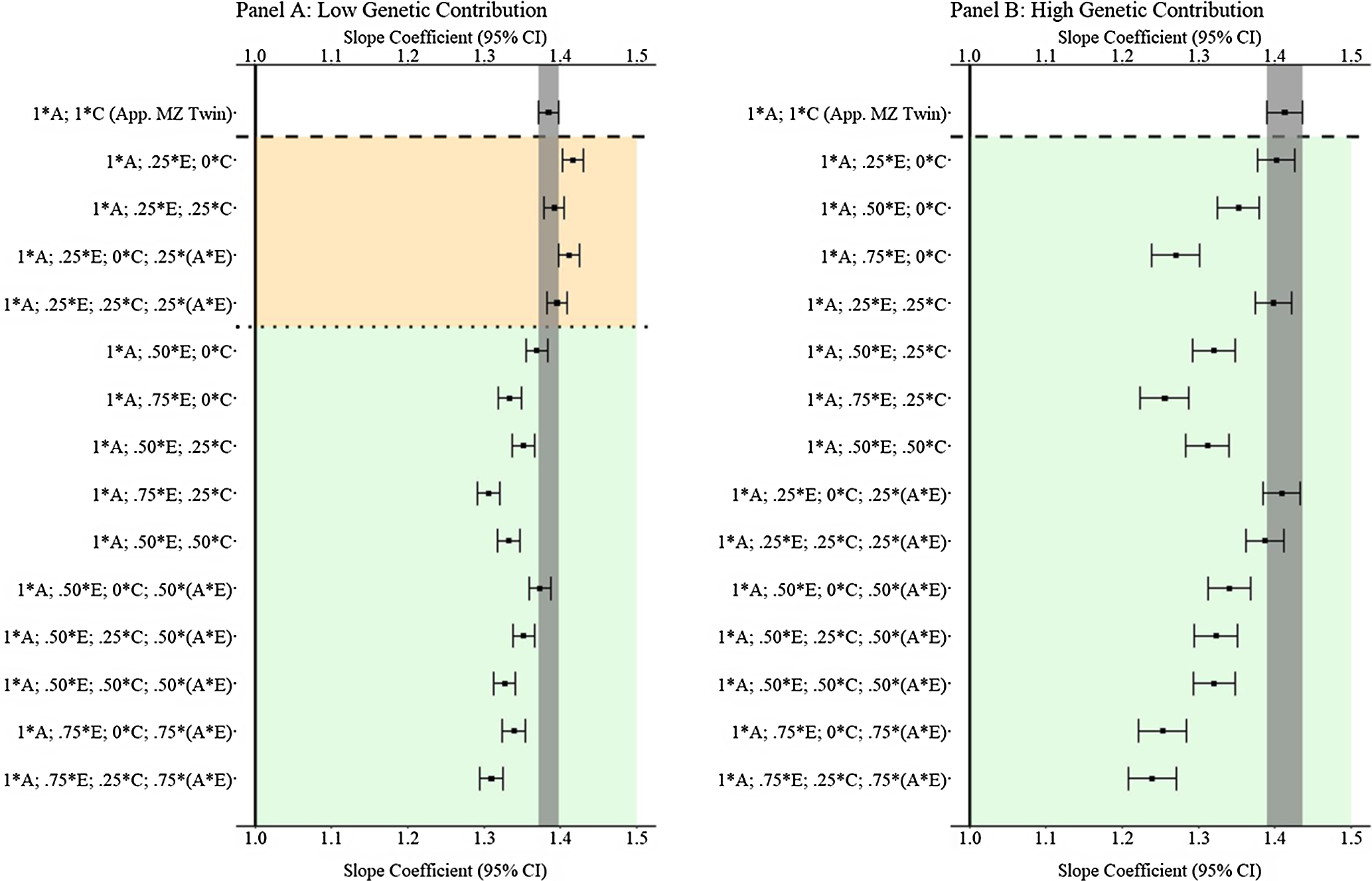
Fig. 10. (Example 2). Slope coefficients of Y regressed on X with low and high genetic contribution to the variation in X .
Note: A = genetics, E = nonshared environment, C = shared environment. The true association between Y and X is 1.00 (Starting N = 10,000). For the current example, Low Genetic Contribution: 8 % genetic, 51.6% nonshared environment, 21.5% shared environment, 14.9% genetic* nonshared environment, and 4% error. High Genetic Contribution: 64 % genetic, 9.6% nonshared environment, 4% shared environment, 18.4% genetic* nonshared environment, and 4% error. Genetic, shared environmental, and nonshared environmental factors equally contributed to the variation in Y . All estimates were derived from a postmatching OLS model. Matching was completed using nearest neighbor matching with a caliper of .05. The orange area provides the specifications that performed further away from the true point estimate (1.00) than the approximation of discordant MZ twin methods, and the green area provides the specifications that were closer to the true point estimate (1.00) than the approximation of discordant MZ twin methods. The proportions on the y-axis represent the proportion of the variation in X contributed by the specified component (A, C, or E) that is adjusted for by the model.
Example 3: Interactions Between a and E, and a and C
The final example, Example 3, demonstrates how estimates using GAPS matching compare the estimates derived from discordant MZ twin methods with two confounding GxE interactions. A proportion of the variation in
X
was specified to be attributed to the interactions between genetic factors and the nonshared environment, and genetic factors and the shared environment. The variation in
X
for Example 3 was specified as
 ${\bf{X}} = { .270_{\bf{A}}} + { .306_{\bf{E}}} + { .102_{\bf{C}}} + { .167_{({\bf{A}}*{\bf{E}})}} + { .116_{({\bf{A}}*{\bf{C}})}} + { .040_{{\bf{rv}}}}$
.
${\bf{X}} = { .270_{\bf{A}}} + { .306_{\bf{E}}} + { .102_{\bf{C}}} + { .167_{({\bf{A}}*{\bf{E}})}} + { .116_{({\bf{A}}*{\bf{C}})}} + { .040_{{\bf{rv}}}}$
.
Results
Figure 11 provides the results of the postmatching estimates. Consistent with Example 1, the estimates derived from the approximation of discordant MZ twin approach were closer to the specified slope coefficient than approximately half of the estimates produced with the GAPS matching approach. The divergent findings between Example 2 and Example 3 highlight that discordant MZ twin methods capture (as specified) more variation in X associated with the shared environment than the nonshared environment. Importantly, the results of Example 3 further demonstrate that the likelihood of producing estimates similar to discordant MZ twin methods increases as more variation in X is captured within the GAPS. Additionally, capturing variation in X attributed to G × E can potentially enhance the likelihood of GAPS matching producing slope coefficients similar to discordant MZ twin methods or being closer to the specified slope coefficient than discordant MZ twin methods.
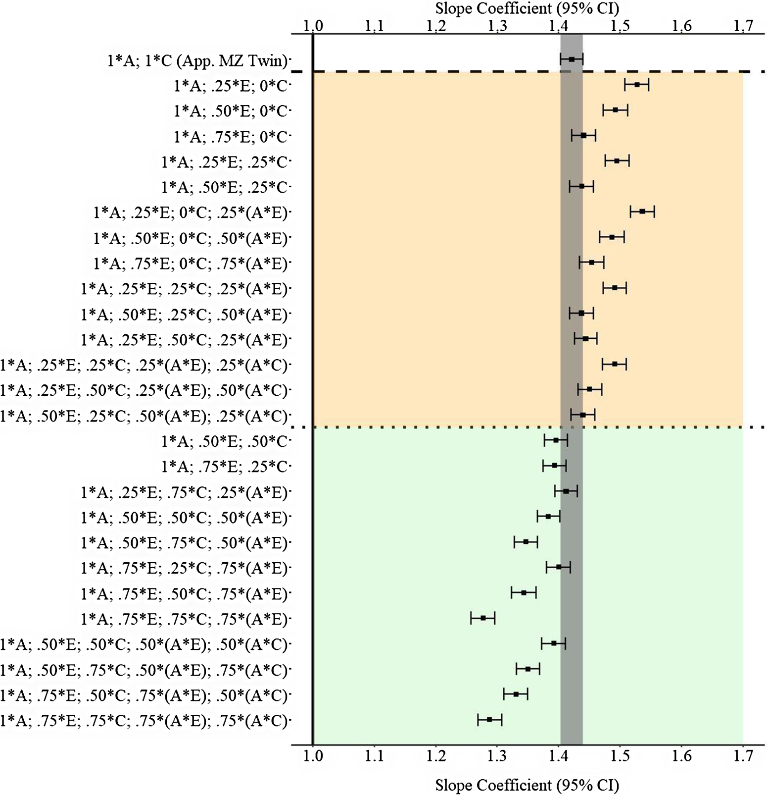
Fig. 11. (Example 3). Slope coefficients of Y regressed on X differentially adjusting for the confounding influence of genetic, shared environmental and nonshared environmental effects.
Note: A = genetics, E = nonshared environment, C = shared environment. The true association between Y and X is 1.00 (Starting N = 10,000). For the current example, variation in X was specified as 27 % genetic, 30.6% nonshared environment, 10.2% shared environment, 16.7% genetic* nonshared environment, 11.6% genetic*shared environment and 4% error. Genetic, shared environmental and nonshared environmental factors equally contributed to the variation in Y . All estimates were derived from a postmatching OLS model. Matching was completed using nearest neighbor matching with a caliper of .05. The orange area provides the specifications that performed further away from the true point estimate (1.00) than the approximation of discordant MZ twin methods, and the green area provides the specifications that were closer to the true point estimate (1.00) than the approximation of discordant MZ twin methods. The proportions on the y-axis represent the proportion of the variation in X contributed by the specified component (A, C or E) that is adjusted for by the model. For example, .25 * E indicates that 7.7% of the variation of X (attributed to the nonshared environment) is adjusted for in the model.
Results from low and high genetic contribution comparisons
In addition to the primary findings of Example 3, comparisons with low (
 ${\bf{X}} = { .060_{\bf{A}}} + { .516_{\bf{E}}} + { .172_{\bf{C}}} + { .149_{({\bf{A}}*{\bf{E}})}} + { .063_{({\bf{A}}*{\bf{C}})}} + { .040_{{\bf{rv}}}}$
) and high (
${\bf{X}} = { .060_{\bf{A}}} + { .516_{\bf{E}}} + { .172_{\bf{C}}} + { .149_{({\bf{A}}*{\bf{E}})}} + { .063_{({\bf{A}}*{\bf{C}})}} + { .040_{{\bf{rv}}}}$
) and high (
 ${\bf{X}} = { .480_{\bf{A}}} + { .0096_{\bf{E}}} + { .032_{\bf{C}}} + { .184_{({\bf{A}}*{\bf{E}})}} + { .168_{({\bf{A}}*{\bf{C}})}} + { .040_{{\bf{rv}}}}$
) genetic contributions to
X
are provided in Figure 12. The results illustrated that GAPS matching can produce estimates similar to discordant MZ twin methods when more than 50% of the variation in genetic, shared environmental and nonshared environmental factors is used to create the GAPS. Nevertheless, at high genetic contributions, when G × E exist for both the shared and nonshared environment, the likelihood of GAPS matching producing estimates similar to the discordant MZ twin estimates is diminished. The divergence is likely a function of the increased ability of the discordant MZ twin approach to adjust for interactions between genetic and shared environmental factors.
${\bf{X}} = { .480_{\bf{A}}} + { .0096_{\bf{E}}} + { .032_{\bf{C}}} + { .184_{({\bf{A}}*{\bf{E}})}} + { .168_{({\bf{A}}*{\bf{C}})}} + { .040_{{\bf{rv}}}}$
) genetic contributions to
X
are provided in Figure 12. The results illustrated that GAPS matching can produce estimates similar to discordant MZ twin methods when more than 50% of the variation in genetic, shared environmental and nonshared environmental factors is used to create the GAPS. Nevertheless, at high genetic contributions, when G × E exist for both the shared and nonshared environment, the likelihood of GAPS matching producing estimates similar to the discordant MZ twin estimates is diminished. The divergence is likely a function of the increased ability of the discordant MZ twin approach to adjust for interactions between genetic and shared environmental factors.
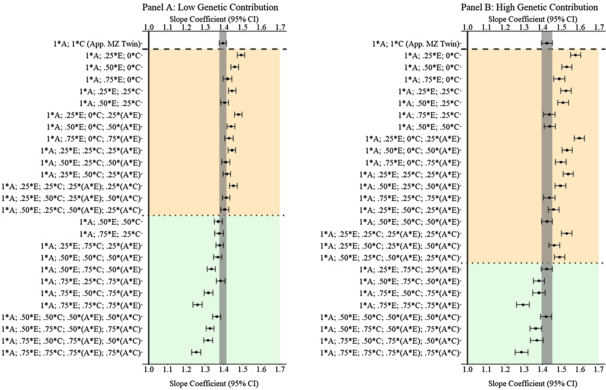
Fig. 12. (Example 3). Slope coefficients of Y regressed on X with low and high genetic contribution to the variation in X .
Note: A = genetics, E = nonshared environment, C = shared environment. The true association between Y and X is 1.00 (Starting N = 10,000). For the current example, Low genetic contribution: 6% genetic, 51.6% nonshared environment, 17.2% shared environment, 14.9% genetic* nonshared environment, 6.3% genetic*shared environment and 4% error. High genetic contribution: 48% genetic, .96% nonshared environment, 3.2% shared environment, 18.4% genetic* nonshared environment, 16.8% genetic*shared environment and 4% error. Genetic, shared environmental and nonshared environmental factors equally contributed to the variation in Y . All estimates were derived from a postmatching OLS model. Matching was completed using nearest neighbor matching with a caliper of .05. The orange area provides the specifications that performed further away from the true point estimate (1.00) than the approximation of discordant MZ twin methods, and the green area provides the specifications that were closer to the true point estimate (1.00) than the approximation of discordant MZ twin methods. The proportions on the y-axis represent the proportion of the variation in X contributed by the specified component (A, C or E) that is adjusted for by the model.
Real Data Example
Sample
To demonstrate the GAPS matching technique using a real data example, a simple analytical evaluation of the association between completing 4 years of college (Wave 3; 0 = did not complete 4 years of college; 1 = did complete 4 years of college) and personal earnings at Wave 4 (higher values represent higher earnings) was conducted. To conduct this demonstration, the current study relied on the restricted version of the National Longitudinal Survey of Adolescent to Adult Health (Add Health). Briefly, the Add Health is a nationally representative sample of individuals from the USA who were in 7th–12th grade during the 1994–1995 school year. Thus far, there have been five waves of data collection between 1994 and 2019. The Add Health is ideal for the current demonstration as it includes (1) oversampled MZ twin pairs (N pairs = 307; N = 614), (2) molecular genetic information from a large portion of the initial sample and (3) a comprehensive survey asking a variety of questions about the shared and nonshared environments. From the initial sample, three subsamples were created. First, a full analytical sample was created using listwise deletion across the two variables of interest (N = 11,587). Second, a GAPS matched subsample was created using listwise deletion, as well as 10 environmental covariates and 11 PRSs, to match participants that did complete 4 years of college to individuals who did not complete 4 years of college by Wave 3 (N = 3,045). Finally, an MZ twin subsample was created using listwise deletion (N pairs = 189; N = 378). The data cleaning process for all of the measures and the analytical syntax for the current demonstration is provided as a text file titled ‘Real data example_GAPS R&R.txt’.
Analytical Strategy
After creating the subsamples, three linear regression models were estimated to evaluate the differential effects of completing 4 years of college (Wave 3) on the log of personal earnings (Wave 4) across the full analytical sample, the GAPS matched subsample and the MZ twin subsample. For the GAPS matched subsample, the matching procedure was conducted by regressing college 4 years on 10 environmental covariates and 11 PRSs to estimate a GAPS, after which, the GAPS was used in conjunction with nearest neighbor matching (caliper = .05) to generate a subsample of participants that completed 4 years of college and participants that did not complete 4 years of college with matching GAPS. Regarding the MZ discordance analysis, a sibling comparison model (using only MZ twins) was estimated permitting the observation of the between-family effects of college 4 years on the log of personal income and the within-family effects (the genetically sensitive effects) of college 4 years on the log of personal income (Knopik et al., Reference Knopik, Ndiderhiser, DeFries and Plomin2016).
Results
Table 2 provides the associations between college 4 years by Wave 3 and the log of personal income at Wave 4 estimated using the full analytical sample, the GAPS matched subsample and the sibling comparison model. As illustrated, completing 4 years of college was positively associated with the log of personal earnings (Wave 4) in the full analytical sample (b = .539, p < .05). However, the slope coefficient was attenuated to b = .465 (p < .05) after conducting the GAPS matching procedure. This suggests that adjusting for environmental and genetic factors almost halved the magnitude of the association. In the sibling comparison model, however, the within-family effect was reduced to b = .459 and rendered statistically nonsignificant (p > .05). Overall, these findings reconfirm the results of the simulation analysis that MZ discordance models will generate more conservative estimates than GAPS matching. Such differences are most likely due to the limitations currently associated with PRSs.
Table 2. Estimating the association between completing 4 years of college and personal earnings using the full Add Health sample, the GAPS matched sample and a sibling comparison model
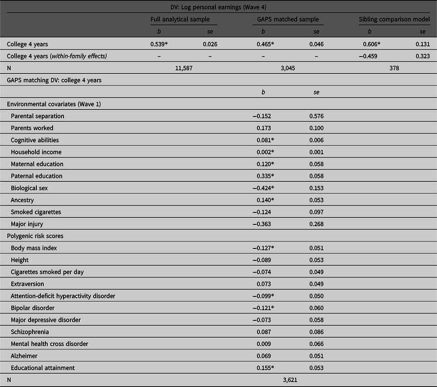
Note: GAPS matching was completed by using a logistic regression model of college 4 years regressed on the specified covariates to estimate a GAPS (predicted probability). After estimating the predicted probability, nearest neighbor matching with a caliper of .05 was completed to create the GAPS matched subsample of 3,315 participants. Listwise deletion was used to create the analytical samples for the current example.
*p < .05.
Discussion
Discordant MZ twin methods currently represent one of the foremost statistical tools for producing nongenetically confounded estimates in the behavioral sciences (Vitaro et al., Reference Vitaro, Brendgen and Arseneault2009). As such, the current study discussed an alternative approach that could potentially produce estimates similar to those of the discordant MZ twin methods. The alternative approach, GAPS matching, integrates variation attributable to environmental risk with variation attributed to genetic risk to adjust estimates for the potential confounding influence of genetic, shared environmental and nonshared environmental factors. The ability of GAPS matching to produce estimates comparable to discordant MZ twin methods was evaluated using 240 simulation analyses. The results from nine of these simulation analyses were reviewed to assess if GAPS matching could approach the estimates produced by discordant MZ twin methods when examining the association between a complex trait ( X ) and an outcome ( Y ). Overall, two findings from the simulated analyses and real data demonstration should be highlighted.
First, when more variation in X was captured by GAPS, the estimates derived from the postmatching regression models generally appeared to be close to or better than the slope coefficients produced by discordant MZ twin methods. The GAPS matching slope coefficients commonly had 95% confidence intervals that overlapped with the 95% confidence intervals of the slope coefficients produced by discordant MZ twin methods. Moreover, the results also illustrated conditions in which GAPS matching could produce a slope coefficient closer to the specified slope coefficient than the discordant MZ twin approach. This finding suggests that GAPS matching can potentially be a useful technique when discordant MZ twin methodologies cannot be employed to examine the research question of interest (e.g., when genomic data are available, but MZ twins are not).
Second, it appears that the confounding influence of an interaction between genetic and nonshared environmental factors was better adjusted for by GAPS matching than discordant MZ twin methods. Given that genetic and nonshared environment interactions contribute to between-individual differences on complex traits in the population (e.g., Purcell, Reference Purcell2002; Knopik et al., Reference Knopik, Ndiderhiser, DeFries and Plomin2016), the ability to adjust for G × E represents an important and potentially substantive advancement of GAPS matching when estimating associations between human phenotypes. Through the reliance on PRSs, GAPS matching can provide the opportunity to statistically adjust for confounding variation associated with interactions between genetic and environmental factors in a way that is not possible using the discordant MZ twin approach (e.g., Schmitz & Conley Reference Schmitz and Conley2017).
Overall, these two key findings demonstrate that the GAPS matching approach can be a promising analytical tool to approximate the estimates produced by discordant MZ twin methodologies. Furthermore, GAPS matching provides the opportunity to test research questions that cannot be assessed using discordant MZ twin methodologies. For instance, GAPS matching can be used to examine the effects of biological sex on psychological outcomes. Additionally, the ability to adjust estimates for G × E is one potential advancement that cannot be achieved when employing discordant MZ twin methodologies. As such, GAPS matching appears to be an analytical strategy that can potentially enhance our understanding of estimated associations.
Limitations of GAPS Matching
Limitations accompanying polygenic scores can diminish the ability to estimate a true GAPS (i.e., their genetic and environmental likelihood). The most influential limitation is the missing heritability problem (Slatkin, Reference Slatkin2009). As evident by heritability estimates derived from GWAS and the real data evaluation conducted in the current study, polygenic scores rarely explain the amount of variation in a phenotype projected by twin-based heritability studies (Manolio et al., Reference Manolio, Collins, Cox, Goldstein, Hindorff, Hunter, McCarthy, Ramos, Cardon, Chakravarti, Cho, Guttmacher, Kong, Kruglyak, Mardis, Rotimi, Slatkin, Valle, Whittemore and Visscher2009). While various factors likely contribute to missing heritability (e.g., Zuk et al., Reference Zuk, Hechter, Sunyaev and Lander2012; Zuk et al., Reference Zuk, Schaffner, Samocha, Do, Hechter, Kathiresan, Daly, Neale, Sunyaev and Lander2014), scholars often suggest that the missing heritability is equated to the inability to achieve enough statistical power (Bloom et al., Reference Bloom, Ehrenreich, Loo, Lite and Kruglyak2013; van der Sluis et al., Reference Van Der Sluis, Verhage, Posthuma and Dolan2010). As demonstrated in Example 1, the missing heritability in polygenic scores limits the capacity of GAPS to capture genetic confounding as well as the MZ difference approach.
In addition to missing heritability, PRSs only capture the effects of common variants on a phenotype and do not capture variation related to the mechanisms influencing specific genetic effects (Purcell et al., Reference Purcell, Wray, Stone, Visscher, O’Donovan, Sullivan and Sklar2009). As such, the inclusion of a PRS does not permit GAPS matching to adjust estimates for the influence of rare variants, structural variation and epigenetics on the association between a phenotype and an outcome (Dudbridge, Reference Dudbridge2013; Wray et al., Reference Wray, Lee, Mehta, Vinkhuyzen, Dudbridge and Middeldorp2014). Although the effects of missing heritability and other limitations of PRSs on GAPS matching appears to diminish the value of the technique, other research teams have begun to produce scores with heritability estimates approaching estimates produced from twin-based heritability studies (Young, Reference Young2019). Moreover, scholars are currently developing strategies to capture variation pertaining to the mechanisms causing specific genetic effects when calculating PRSs, including the identification of rare variants (Crouch & Bodmer, Reference Crouch and Bodmer2020) and biologically informed polygenic scores (Hari Dass et al., Reference Hari Dass, McCracken, Pokhvisneva, Chen, Garg, Nguyen, Wang, Barth, Yaqubi, McEwen, MacIsaac, Diorio, Kobor, O’Donnell, Meaney and Silveira2019). As such, if the analytical sample and techniques for GWAS and polygenic scores continue to advance, the effects of missing heritability and the inability to quantify the mechanisms causing specific genetic effects on the estimates produced by GAPS matching should be diminished (Young, Reference Young2019).
Limitations of the Simulation Analyses
In addition to the limitations associated with GAPS matching, the current simulation was tasked with comparing a twin-based statistical methodology to a methodology designed for singletons. As such, while matching represented the foremost strategy to potentially compare the discordant MZ twin approach to the GAPS matching approach, the simulation analysis was limited in developing matched ‘twin’ pairs — pairs matched using A and C — that were identical. As such, future scholarship should employ real twin data with genomic data to compare the methodologies and provide an approximation of the bias present in the GAPS approach due to the limitations associated with polygenic scores. Moreover, the comparisons on the simulated datasets conducted using the 95% confidence intervals are subject to the limitations associated with frequentist probability theory (Fox, Reference Fox2016; Law, Reference Law2015). As such, we believe it would be unwise to compare these approaches using the 95% confidence intervals when applying the approach to real data given that twin samples and samples of singletons with molecular genetic information can be structurally different. Additionally, due to difficulties specifying a simulation where the resulting dataset is representative of both twins and singletons, the current study relied on the assumption that the matching error rate would be identical when conducting GAPS matching and difference score analyses using MZ twins. Due to this assumption, the estimates resulting from the discordant MZ twin approach are likely upwardly biased because of the relatively low rate of misidentification associated with MZ twin pairs (Knopik et al., Reference Knopik, Ndiderhiser, DeFries and Plomin2016). As such, future research should consider this limitation when implementing the GAPS matching approach in an effort to more closely emulate discordant MZ twin models.
Conclusion
Long considered the foremost statistical approach to producing nongenetically confounded estimates, discordant MZ twin methodologies provide a unique opportunity to adjust estimates for the confounding influence of genetic and shared environmental factors. The simulation analyses conducted in the current study illustrated the robust nature and validity of discordant MZ twin methodologies. Challenges associated with the discordant MZ twin approach, however, remain. Considering these challenges, the GAPS matching approach was discussed, and simulation and real data analyses were conducted to compare the estimates produced using the GAPS matching approach to the estimates produced using the discordant MZ twin approach. While the simulations illustrated favorable findings, current challenges associated with GAPS matching — illustrated in the real data example — hinder the ability for users to estimate slope coefficients similar to the slope coefficients produced using discordant MZ twin methodologies in all conditions. Nevertheless, as missing heritability diminishes and rich survey data is collected alongside whole genome data, GAPS matching could present a unique opportunity to approximate or advance upon discordant MZ twin methodologies.
Acknowledgments
The authors want to thank J.C. Barnes for his insight into conducting the simulation analyses.


 Open access