


INTRODUCTION
A leading explanation for sudden ice-shelf disintegration, as exemplified by the 2002 breakup of the Larsen B, involves the effects of atmospheric warming, increased surface melting and the creation of an impermeable ice-shelf surface that retains large volumes of meltwater which eventually drives hydrofracture (Scambos and others, Reference Scambos, Hulbe, Fahnestock and Bohlander2000). According to the theory, surface and englacial warming, extended melt seasons and increased down-slope wind conditions gradually turn the thermally protective firn layer into a bare-ice surface that resists meltwater infiltration (e.g. van den Broeke, Reference van den Broeke2005; Holland and others, Reference Holland2011; Trusel and others, Reference Trusel2015; Hubbard and others, Reference Hubbard2016; Lenaerts and others, Reference Lenaerts2017). Build-up of surface meltwater storage capacity (e.g. Glasser and Scambos, Reference Glasser and Scambos2008; Banwell and MacAyeal, Reference Banwell and MacAyeal2015; Kingslake and others, Reference Kingslake, Ely, Das and Bell2017) and interruption of flow features, like rivers and streams, that can remove meltwater volume (Banwell, Reference Banwell2017; Bell and others, Reference Bell2017), may eventually lead to hydrofracture-driven fragmentation of the ice shelf (e.g. Scambos and others, Reference Scambos, Hulbe, Fahnestock and Bohlander2000, Reference Scambos2009; Banwell and others, Reference Banwell, MacAyeal and Sergienko2013; Macdonald and others, Reference Macdonald, Banwell and MacAyeal2018).
Understanding ice-shelf disintegration, and the ability to anticipate it in the future, requires reliable methods to observe surface and subsurface melting. Unlike the ablation zones in Greenland, where steep surface topography drives immediate movement of meltwater as it is created, flat ice-shelf surfaces allow surface and subsurface meltwater to build-up in bog-like areas where the topography is subtle, but heterogeneous (Banwell and others, Reference Banwell2014). Flat surface topography and the absence of firn also promotes subsurface melting driven by solar radiation that penetrates the surface (Leppäranta and others, Reference Leppäranta, Jarvinen and Mattila2012; Jarvinen and Leppäranta, Reference Jarvinen and Leppäranta2013; Lenaerts and others, Reference Lenaerts2017). While the collapse of the Larsen B Ice Shelf in 2002 was preceded by a well-developed surface expression of meltwater (Sergienko and MacAyeal, Reference Sergienko and MacAyeal2005; Glasser and Scambos, Reference Glasser and Scambos2008), the collapse of the Wilkins Ice Shelf in 2008 was attributed to the presence of water below the surface that enabled hydrofracture (Scambos and others, Reference Scambos2009). The processes allowing development of subsurface water ponding are thus pertinent to ice-shelf stability.
Over a 3-year period from 2015 to 2017, we conducted a ground-based study of surface meltwater features on the ablating portion of the McMurdo Ice Shelf (McMIS), Antarctica (Fig. 1). One objective of the study was to determine the ice-shelf flexure/fracture response associated with surface water ponding and drainage. A second objective of the study, which we report here, was to determine the seismic signals associated with the water ponding and movement. The heterogeneous nature of the surface topography, albedo and debris cover, coupled with meters-thick subsurface meltwater and slush layers (e.g. Paige, Reference Paige1968; Klokov and Diemand, Reference Klokov and Diemand1995), made access to the field area and optimal instrument placement virtually impossible (Fig. 2). Because of these difficulties, our seismometer deployment scheme was modest, restricted to two locations and extended for 63 days at the onset of the 2016/17 melt season (Fig. 1).
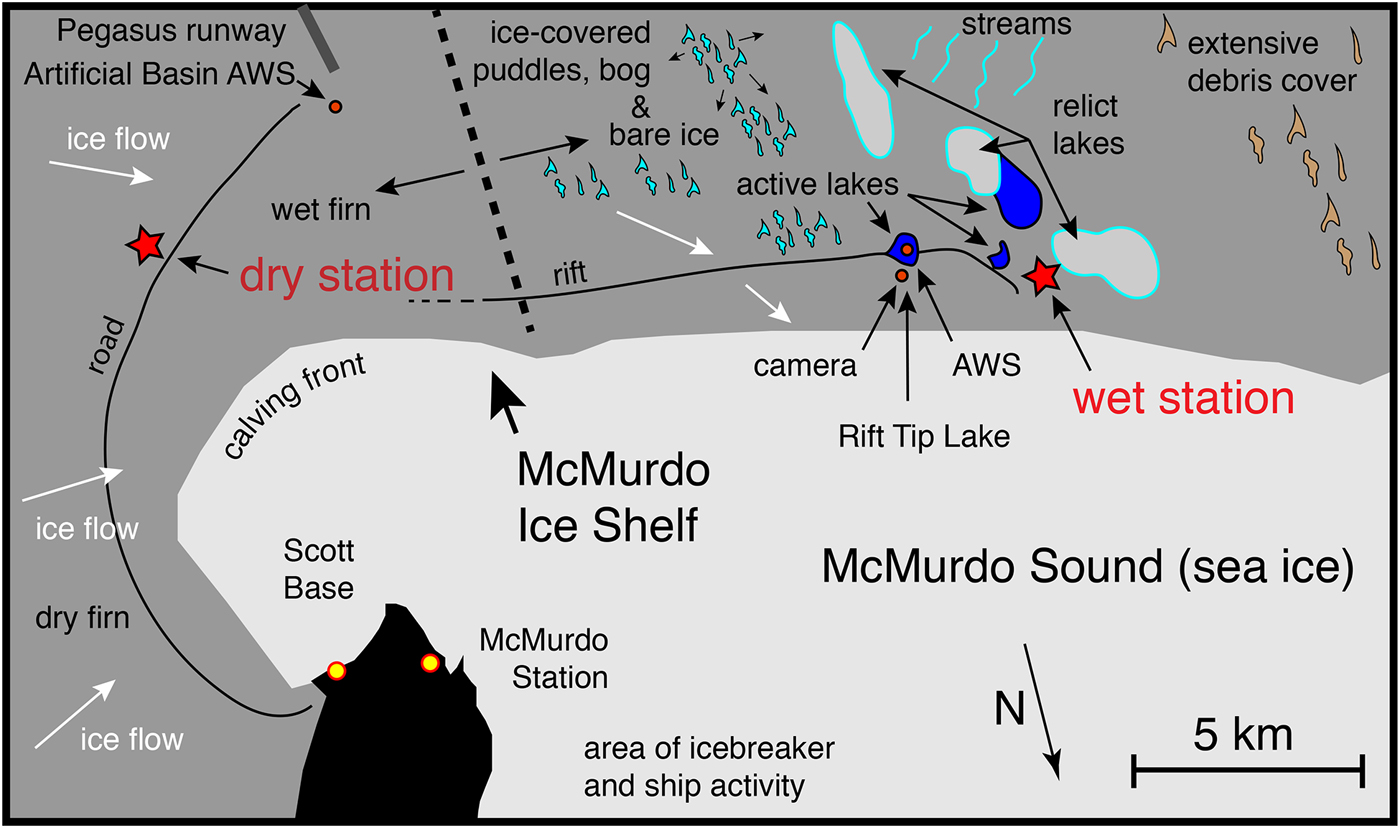
Fig. 1. Field setting and location of instrumentation. The seismometer deployed at the ‘dry station’ is in a conventional, firn-covered ice-shelf area of ~50 m thickness. The seismometer deployed at the ‘wet station’ is in a region of bare ice and (some) debris cover displaying complex surface meltwater features including surface and subsurface lakes, ephemeral surface ponds with ephemeral ice cover, streams, and ‘relict’ surface lakes that had open water in previous years. Ice thickness at the wet station is ~25 m.
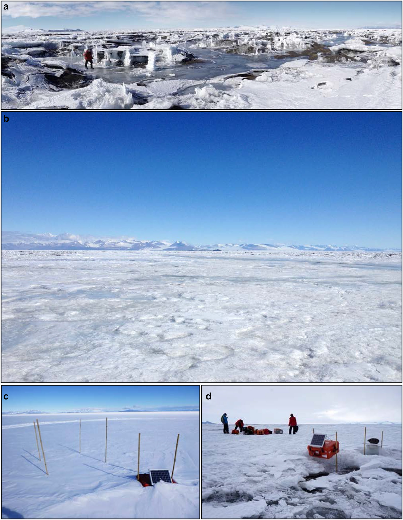
Fig. 2. Photographs of the McMIS surface melt zone taken in December and January. (a) Surface lake near the wet station (28 January 2017). (b) Bog-like conditions near Rift Tip Lake (17 December 2015). (c) Seismometer deployment at the dry station (23 November 2016). (d) Seismometer deployment at the wet station (20 November 2016).
Previous deployment of seismometers on, or adjacent to, floating ice shelves, has been exclusive to cold, firn-covered accumulation zones where surface temperatures are colder than freezing for most, or all, of the year (Podolskiy and Walter, Reference Podolskiy and Walter2016). These previous deployments have focussed primarily on aspects of ice/ocean interaction that give rise to seismic signals, such as flexural wave propagation (Hatherton and Evison, Reference Hatherton and Evison1962), ocean gravity-wave forcing (Cathles and others, Reference Cathles, Okal and MacAyeal2009; Bromirski and others, Reference Bromirski, Sergienko and MacAyeal2010; Bromirski and Stephen, Reference Bromirski and Stephen2012), rift propagation (Bassis and others, Reference Bassis2007; Banwell and others, Reference Banwell2017), tidally modulated stick-slip earthquakes and slip tremor at grounding lines (e.g. Winberry and others, Reference Winberry, Anandakrishnan, Wiens and Alley2013; Lipovsky and Dunham, Reference Lipovsky and Dunham2016), vertical stratification of seismic and hydro-acoustic properties (Zhan and others, Reference Zhan, Tsai, Jackson and Helmberger2014; Diez and others, Reference Deiz2016) and tidal flexure (e.g. Hulbe and others, Reference Hulbe2016). Where these studies have addressed glacial hydrologic processes, the majority have been focussed on subglacial hydrology (e.g. Walter and others, Reference Walter, Deichmann and Funk2008; Winberry and others, Reference Winberry, Anandakrishnan and Alley2009). The present study joins a few other recent cryoseismological efforts (e.g. Chaput and others, Reference Chaput2018; MacAyeal, Reference MacAyeal2018; Podolskiy and Others, Reference Podolskiy, Fujita, Sunako, Tsushima and Kayastha2018) in attempting to characterize surface conditions such as melting, freezing and changing temperature using seismological methods and data.
FIELD SETTING
The McMIS occupies an embayment surrounded by the mountainous Ross Island Archipelago and is neighbored by the dry-valleys of the Royal Society Range to the West, the Ross Ice Shelf to the South and East, and the McMurdo Sound, into which it flows, to the North (e.g. see Fig. 2 of Dunbar and others (Reference Dunbar, Bertler and McKay2009)). Both the US McMurdo Station and N.Z. Scott Base are located proximal to our field area. Ice flow of the McMIS is primarily from East to West, traversing a strong micro-climate gradient that extends from the firn-covered Ross Ice Shelf, which rarely has a surface temperature above 0°C, to a zone of strong surface ablation made possible by down-slope winds coming over Mount Discovery and Minna Bluff (e.g. Kuipers Munneke and others, Reference Kuipers Munneke2018). The Western end of the McMIS is covered with wind-blown terrigenous debris (Glasser and others, Reference Glasser, Goodsell, Copland and Lawson2006) and marine sediment derived from basal freezing and anchor ice deposition (Debenham, Reference Debenham1965; Swithinbank, Reference Swithinbank1970; Kellogg and Kellogg, Reference Kellogg and Kellogg1987). The presence of convoluted medial moraines on the Western McMIS, suggests that the McMIS is largely a relict of a once more widespread ice shelf filling McMurdo Sound (Glasser and others, Reference Glasser, Goodsell, Copland and Lawson2006).
The microclimate gradient and the increasing presence of supraglacial debris (a combination of windblown dust and marine material brought up from the ice-shelf bottom) lead to a major transition from cold, firn-covered ice shelf in the East, to bare-ice/debris-covered surfaces in the West. This transition also involves a change in the surface hydrology: first, a surface that is mottled with puddles and slush-filled depressions that are typically covered by thin frozen ice lids (Paige, Reference Paige1968; Klokov and Diemand, Reference Klokov and Diemand1995); second, a region of surface ‘bogs’ and lakes within patches of debris; and third, an area of numerous incised sub-parallel surface streams and rivers (Figs 1 and 2).
INSTRUMENTATION AND DATA CHARACTERISTICS
The two seismometer stations were deployed ~ 20 km apart on either side of the transition between firn-covered and bare/melting ice-shelf surface, and so we refer to them as the ‘dry station’ and the ‘wet station’ (Fig. 1). Both stations were equipped with broadband instruments (Nanometrics T120), and the wet station was additionally equipped with two 3-component short-period geophones (Sercel L28). The instruments operated autonomously from mid-November 2016 to late January 2017 (Table 1). The dry station's single instrument was deployed in a dry snow pit 30 cm below the surface, adjacent to a heavily travelled over-snow road to Pegasus runway. Three instruments at the wet station were deployed in a 1 m deep hole in the bare-ice surface. Due to uncertainty about how the instruments would behave in a wet, ice-shelf ablation zone and concern about widespread flooding, all three instruments of the wet station were deployed within a 5 m2 area.
Table 1. Instrumentation

* Hydroacoustic noise generated by ship operations in McMurdo Sound dominated the data from 15 January 2017 onward.
The Nanometrics T120 seismometers have an instrument response function that is ideal (‘flat’ Bode diagram with amplitude near unity and phase near zero) for periods from 120 s to frequency 100 Hz (see https://www.passcal.nmt.edu). Data from the T120s was dominated by sub 1 Hz sea swell, buoyancy oscillations (ice-shelf bobbing and rocking), impulsive surface gravity waves from nearby calving and iceberg capsize, and teleseisms from distant earthquakes (Lin, Reference Lin2017). The L28s have an instrument response function that is ideal from ~ 5 Hz to > 500 Hz (again, featuring a ‘flat’ Bode diagram with amplitude near unity and phase near zero, see https://www.passcal.nmt.edu). The L28 instrument response is also ideal for the observation of icequake activity, which is the main emphasis in this study, because it naturally high-pass filters the ground motion to eliminate the sub 1 Hz signal that dominates the record observed by the T120s. A preliminary display of data, high-pass filtered (passing frequencies above 10 Hz), collected by the two T120s operating at each station is provided in Fig. 3 for an 18-day period. The T120 data are high-pass filtered to eliminate the dominant sea-swell signal at frequency ~ 1 Hz and below, and to reveal the diurnal pattern of seismicity (appearing in the top panel of Fig. 3 representing the wet station) to be discussed below. While the data were easily corrected for instrument response, no elements of the analysis presented here involved signals that were outside of the ideal response range of the sensors (‘flat’ Bode diagram with amplitude near unity and phase near zero). Because the T120s were the only common sensors between the two stations, comparisons between the two stations were done with T120 data. When analyzing the diurnal seismicity cycle (see the following sections) at the wet station, data from the L28s was used because their instrument response naturally suppressed sub 1 Hz sea swell.

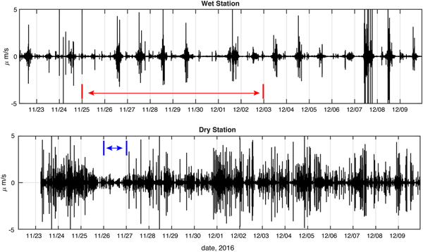
Fig. 3. Comparison of ground velocity (μm s−1) seismograms (100 sample per second vertical HHZ channel high pass filtered to > 10 Hz; both collected using T120 broadband seismometers, Table 1) for the wet (top panel) and dry stations (bottom panel) over the 18-day period in late November to early December 2016, when differences between the two stations were most apparent (time measure is UTC). The wet station displays a repeating diurnal pulse of seismicity (~6–12 hr in length), and this forms the focus of interest in the present study. The dry station is much noisier due to a predominance of anthropogenic signals from a nearby over-snow road and airfield. The minimum in signal level from 26 to 27 November (blue span lower panel) corresponds to the Thanksgiving holiday (station recess from work activity) for McMurdo Station, when the anthropogenic noise was reduced. The 8-day period over which the standard deviation of the wet and dry ground velocities are compared in Fig. 5 is indicated in red on the upper panel.
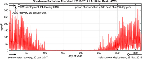
Other instruments (see Table 1) involved in our project included two automatic weather stations (AWS), one deployed for a full-year at a site called Artificial Basin (Fig. 1), and another operated for 3 months at Rift Tip Lake during the period of seismometer operation (Fig. 1). The AWS data provide air temperature and net shortwave radiation measurements at 2 m above the surface for comparison with the seismic data. GPS instruments were also deployed in the area, which recorded tidal elevation data for comparison with the seismic data (see below).
COMPARISON: WET VS. DRY ICE-SHELF SEISMICITY
Figure 3 displays high-pass filtered (> 10 Hz) vertical ground velocity seismograms for the wet and dry stations over an 18-day subset (22 November--10 December) of the 63-day total observation window, when the differences between the wet and dry ice-shelf seismicity were most apparent. The wet station's ground motion (top panel, Fig. 3) displays a diurnally repeating, ~ 6–12 hr-long, period of increased seismicity that forms the central focus of interest in this study. This period occurred during the local evening. Following 10 December (not shown in Fig. 3), the diurnal seismicity was intermittent and sometimes absent for days. The pattern of diurnal seismicity is not seen in the dry station's seismogram (bottom panel, Fig. 3).
Inspection of the event waveforms in the two stations (Fig. 4) suggests that the events composing the wet station's diurnal seismic signal are generated primarily by natural sources which have small spatial and temporal scales (judging from < 1 s duration and frequency content of the events). In contrast to the short seconds-scale duration of events at the wet station, the majority of signals observed at the dry station are on the order of tens of minutes in duration. This probably reflects anthropogenic sources related to vehicle traffic on the over-snow road located ~ 100 m from the seismometer vault, and possibly also to activity at the McMurdo Station airstrip on the dry part of the McMIS (Williams Field), ~ 4 km distant. The wet station is separated by ~ 20 km from the dry station and associated anthropogenic activity, so the data show no corresponding anthropogenic signals except in late January when hydroacoustic tremor generated in McMurdo Sound by a US Coast Guard icebreaker and the ships it escorted is observed.

Fig. 4. Example waveforms (100 sample per second HHZ channel, high pass filtered > 10 Hz) for the wet (top panel) and dry (bottom panel) stations. Typical signals at the wet station are sub-second in duration and exhibit frequencies well above 10 Hz. In contrast, the dry station exhibits emergent tremor signals that last for tens of minutes with quasi-symmetric amplitude envelopes suggestive of passing vehicles on the nearby road.
To quantitatively investigate the difference between the dry- and wet-station signals, we computed the standard deviation of each station's vertical ground motion evaluated over 60-second time segments and then used a 20-minute running mean to provide a relatively smooth proxy record for event density and seismicity (we shall refer to this proxy record as ‘seismicity’ from this point on). An alternative measure of seismicity, which identifies and counts individual icequakes and other events is developed below in a discussion of how event number varies with amplitude. Both measures of seismicity were found to identify the diurnal cycle, and the standard deviation proxy is preferable for determining correlations with possible causes.
Figure 5 presents each station's seismicity over an 8-day window (25 November–3 December 2016), chosen as it is representative of the differences between the two stations. Prominent in the seismogram of the wet station is the diurnal cycle identified in Fig. 3. Over the 8-day window shown in Fig. 5, the prominent diurnal peaks are visible on 7 days, but one diurnal peak is conspicuously missing on 30 November. We shall use this missing peak as a crucial test in developing a hypothesis for the cause of the diurnal seismicity.
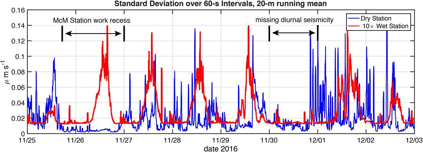
Fig. 5. Standard deviation of ground velocity over 60-second intervals (μm s−1, 100 sample per second HHZ channel high pass filtered to > 10 Hz) for the wet and dry stations over a representative 8-day period at the start of the melt season (time measure is UTC). The data are then smoothed using a 20-minute running mean filter. The wet station's values have been multiplied by 10 to facilitate comparison with the values from the dry station. The wet station has a prominent diurnally repeating pulse of seismicity which appears each day except on 30 November.
Seismicity of the dry station is about an order of magnitude larger in amplitude than that of the wet station, but lacks the prominent diurnally repeating cycle. Although data on local work activity at McMurdo Station and Scott Base were not collected, the peaks and valleys of the dry station's seismicity are consistent with anthropogenic activity on the nearby roads and airfields. In fact, a prominent window of low seismicity is seen from late 25 to early 27 November 2016 in the dry station's record. McMurdo Station celebrated a Thanksgiving holiday work recess during this period. Efforts to find the short-duration, high-frequency events associated with the wet station's diurnal cycle of seismicity in the dry station's record were unsuccessful.
CAUSE OF DIURNAL SEISMICITY AT THE WET STATION
The diurnal pulsation of seismicity observed at the wet station in November and early December, and intermittently from mid-December to mid-January, constitutes the largest difference between the wet and dry station records. The presence of this phenomenon at the wet station, but not at the dry station, is a simple and strong indicator that it is associated with some aspect of ice-shelf melting and surface hydrology.
Diurnal cycles of seismicity on an ice shelf have been observed before, but not in association with ice-shelf melting and surface hydrology. Hulbe and others (Reference Hulbe2016) observed diurnal and semidiurnal pulsations of seismicity on the Ross Ice Shelf near the grounding line of the Kamb Ice Stream that correlated with falling tide and was caused by tidal flexure induced fracture (see Fig. 7 in Hulbe and others, Reference Hulbe2016).
To test whether the diurnal pulsations at the wet station are caused by the tide, we compared the seismicity with the tide observed at a GPS station located 80 m from the seismometer site. The result is shown in Fig. 6. The periods of strong seismicity begin with the rising tide, and seismicity reaches a maximum during the initial period of falling tide. Thus, the mechanism of seismicity generation applicable in the grounding-line situation described by Hulbe and others (Reference Hulbe2016) could be at play on the McMIS. The most conspicuous refutation of a tidal cause, however, is the fact that a diurnal seismicity pulse is absent on 30 November 2016, despite the ocean tide being approximately the same as for the days when the diurnal seismicity pulse was observed.
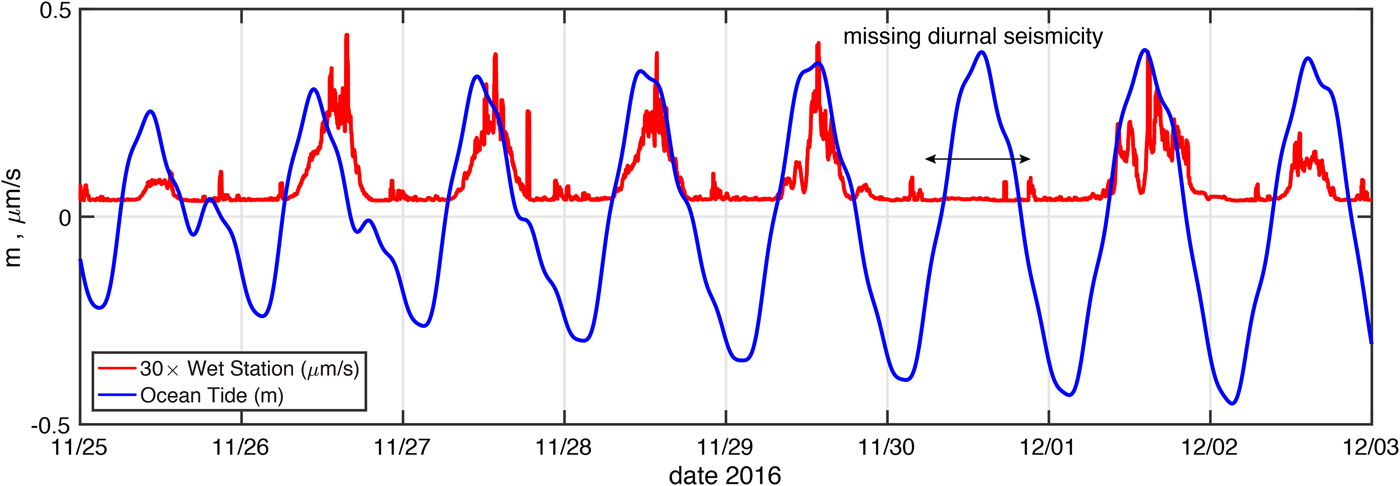
Fig. 6. Comparison of ocean tide elevation (m) and seismicity (μm s−1) at the wet station (see Fig. 5). The absence of diurnal seismicity episode on 30 November 2016 is conspicuous given the relatively strong ocean tide at the time. The wet station's values have been multiplied by 30 to facilitate visual comparison with the tidal elevation. We also note the presence of smaller-amplitude seismicity in the record, typically occurring during the last few hours of each day (UTC time). The focus of our study is on the windows of seismicity of large amplitude which occur during mid-day, i.e., between 11:00 and 18:00 UTC.
We conclude, therefore, that a process associated with ocean tide is not the cause of the diurnal seismicity. We qualify this conclusion by noting that there appear to be other, smaller pulsations of seismicity that occur on a daily basis, most notably during the last 2 hours of the day (UTC time), which could be driven by ocean tide (Fig. 5). These smaller pulses occur just before low tide, so they may reflect some aspect of ice-shelf flexure or other movement (Fig. 6).
In searching for another possible cause of the diurnal seismicity, we found studies which reported diurnal seismicity pulsation below Arctic sea ice, near the floating ice cover of Lake Bonney, Antarctica and in debris-covered alpine glaciers of the Himalaya (Milne, Reference Milne1972; Carmichael and others, Reference Carmichael, Pettit, Hoffman, Fountain and Hallet2012; Podolskiy and others, Reference Podolskiy, Fujita, Sunako, Tsushima and Kayastha2018). In all of these studies, the cause of the seismicity was cited to be plate fracture associated with thermal bending moments on the floating ice cover driven by cooling air temperature. The theory of thermal bending moment induced fracture is described by Evans and Untersteiner (Reference Evans and Untersteiner1971) and Bažant (Reference Bažant1992).
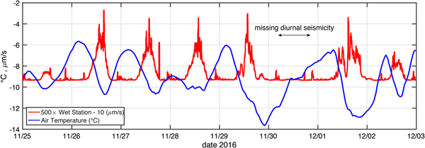
To test this possibility, we compared the seismicity (described above) with the 2-m air temperature measured at an automatic weather station (AWS, data measured every 15 s, and averaged every 15 minutes) located at Rift Tip Lake, ~3 km away from the wet station (Fig. 1). The result is shown in Fig. 7. The comparison reveals that seismicity pulses seem to correspond with the daily cycle of falling air temperature. Most notable in the comparison is the lack of a seismicity pulse on 30 November coinciding with the only day of the 8-day period in which surface temperature did not fall (i.e., the minimum temperature occurs on the day before, and the temperature rises all day to a maximum occurring the following day).

Fig. 7. Comparison of 2-m air temperature (°C, smoothed with a 4-hour running mean filter) with standard deviation of ground motion at the Wet Station (see Fig. 5). The wet station's standard deviation signal has been multiplied by 500 to facilitate comparison with the temperature record. Diurnal seismicity pulses seem to occur at times of falling air temperature except on 30 November when temperature only increased all day.
THERMAL MODEL OF THE ICE SHELF
To investigate further the relationship between diurnal seismicity and air temperature, we created a simple one-dimensional (1-D) (vertical column) numerical model of heat transfer on the McMIS. The purpose of this model is to determine when thermal bending moments on the ice-shelf surface can induce fracture. Key to this model is its ability to simulate subsurface slush/water layers and the development of a centimeters-thick surface ice lid. Thermal bending moments on this lid, and associated fracture are what we propose to be the origin of the diurnal seismicity cycle at the wet station.
The model computes the time-dependent temperature vs. depth profile, T(z, t), using surface temperature, T s(t), and sea-water temperature, T sw, as boundary conditions at the surface, z = z s and base, z = z b, of the ice shelf. The ice shelf is taken to be 25 m thick, although it varies within the field area from 10 to 30 m (Rack and others, Reference Rack, Haas and Langhorne2013; Campbell and others, Reference Campbell, Courville, Sinclair and Wilner2017). The model features solar radiative heating, S(z, t), in the near surface of the ice column. The solar heating is taken from shortwave radiation observations at the Artificial Basin AWS, because its time series is longer than at the Rift Tip Lake AWS, and is assumed to decay with depth below the surface with a skin depth of 0.5 m (Leppäranta and others, Reference Leppäranta, Jarvinen and Mattila2012; Jarvinen and Leppäranta, Reference Jarvinen and Leppäranta2013). When boundary conditions and solar heating allow, the temperature at the surface and in the subsurface can reach the melting point for ice, which we take to be 0°C. The model accounts for latent heat absorption once T = 0°C by changing the water/ice mixing ratio, Q(z, t), which is 0 for all ice and 1 for all water. Because of the small ice-shelf thickness, heat transfer associated with advection driven by strain rate, surface ablation (e.g. Glasser and others, Reference Glasser, Goodsell, Copland and Lawson2006) and basal platelet ice accumulation (e.g. Smith and others, Reference Smith, Langhorn, Frew, Vennell and Haskell2012) are considered second-order effects, and so, for simplicity, only heat conduction associated with shortwave solar absorption is treated here.
A schematic representation of our simple model domain is shown in Fig. 8. In this simple geometry, a frozen lid covers a slushy, water-covered surface when there is sufficient incoming solar radiation to support melting. This concept is based on observations of supraglacial lakes in Dronning Maud Land, Antarctica, in a flat area near a nunatak (Leppäranta and others, Reference Leppäranta, Jarvinen and Mattila2012; Jarvinen and Leppäranta, Reference Jarvinen and Leppäranta2013).
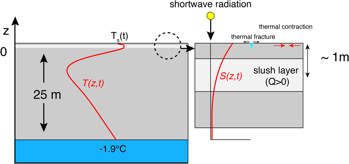
Fig. 8. Schematic depiction of 1-D model domain used for simple thermal modeling. The temperature- depth profile T(z, t) (left side of figure) represents conditions around ~1 January when solar absorption below the surface generates a subsurface meltwater/slush layer. The schematic depiction of solar heating S(z, t) (right side of figure) displays exponential decay with depth below the surface with a skin depth, d, of 0.5 m, which is taken from observations by Jarvinen and Leppäranta (2013).
The governing equation for the temperature-depth profile is
 $$ {\displaystyle{\partial {\cal W}} \over {\partial t}} = k {\displaystyle{\partial^2 T} \over {\partial z^2}} + S(z,t) $$
where t is time, z is the vertical distance (positive upward, 0 at sea level), k = 2.22 W m−1 K−1 is the thermal conductivity of ice, S(z, t) is the solar heating,  ${\cal W}$ is the total heat density (sum of sensible and latent heat) of the ice defined by
 $$ {\cal W}(z,t) = \rho_i \ c \ T(z,t) + \rho_i \ L\ Q(z,t) $$
where T(z, t) is temperature, 0 ≤ Q(z, t) ≤ 1 is water mixing ratio, and ρi = 917 kg m−3, c = 2.05 kJ kg−1 K−1, and L = 334 kJ kg−1 are the density, heat capacity and latent heat of fusion of ice, respectively. Disregarding pressure effects, we take the melting temperature to be constant, 0°C. This then means that
 $$W(z,t) = \left\{ {\matrix{ {\rho _i c\,T(z,t)} & {{\rm if}\quad T \lt 0} \cr {\rho _i\,L\,Q(z,t)} & \,\,{{\rm if}\quad T = 0.} \cr } } \right.$$
To compute T and Q, we use an implicit time-stepping scheme (which is unconditionally stable) with a time-step dt = 30 minutes consistent with the sampling rates of the AWS system providing model forcing data. The vertical resolution of the finite-difference grid, dz, is 3 cm.
At the end of each time step, grid points where T > 0 are adjusted to restore T to 0 by increasing Q by the amount needed to convert the unphysical sensible heat (ρi c T where T > 0) to latent heat (ρi L Q with T = 0). Grid points where Q < 0 are adjusted to restore Q to 0 by decreasing T from the melting point (0°C) to the new temperature T = LQ/c. The water fraction Q is not allowed to exceed 1. When this happens in the model, Q is restored to 1 (at the end of an offending time step) and the extra heat that caused Q to exceed 1 is discarded, as our model is intentionally too simple to account for heat transfer in liquid water layers. Strictly speaking, the adjustments to Q needed to keep it within the [0, 1] interval mean that the model does not conserve energy. Adjustments to prevent Q > 1 were relatively rare and probably acted to reduce the net meltwater production, thus meltwater generation estimates made by the model represent a lower bound.
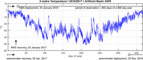
Boundary conditions required by Eqn (1) are the specifications of the basal and surface temperatures. For basal temperature at z = z b, T(z b, t) is constant at T sw = −1.9°C, the melting temperature in saline ocean water (e.g. Smith and others, Reference Smith, Langhorn, Frew, Vennell and Haskell2012). For surface temperature at z = z s, we specify T s = T(z s + 2, t) using a derived annual record of temperature measured 2 m above the ice-shelf surface by the AWS located ~ 12 km away at the Artificial Basin (Table 1, Fig. 1). When T(z s + 2, t) was >0°C, we substituted T s = 0.
To compile the derived annual record, we noted that the AWS at Artificial Basin observed T(z s + 2, t) for 365 days over the period of 24 January 2016 to 22 January 2017 (this was not the case for the AWS at Rift Tip Lake, which was closer to the wet station). The AWS observations covered 364 days of a 365-day year; thus we assigned each day of AWS data to the appropriate day-of-year and interpolated for the one missing day to derive the annual record.
The derived annual record of temperature used to force the model, T s = T(z s + 2, t), is shown in Fig. 9. To account for the temperature difference between the Artificial Basin and the wet station site, located 12 km away, a warming offset, T off = +1°C was added to the 2-m temperature shown in Fig. 9. This offset temperature is the value (rounded to the nearest degree) obtained by comparing the AWS stations at Artificial Basin and Rift Tip Lake. (The AWS at Rift Tip Lake operated only from mid-November 2016 to mid-January 2017, so it could not be used to develop the annual surface-temperature record used by the model.) Sensitivity of the results to this offset temperature is discussed below.

Fig. 9. Temperature (°C) measured 2 m above the ice-shelf surface at Artificial Basin, approximately 18 km from the wet station from 25 January 2016 to 23 January 2017 . This record has been re-expressed as a function of day-of-year for a perpetually repeating 366-day leap year to develop the annual record used as the surface boundary condition for the thermal model. This annual boundary condition record was repeated during model spin-up to eradicate the effects of an arbitrary initial condition. Also shown are time-lines for AWS and seismometer operation relative to the derived annual record.
Solar heating, S(z, t), required by Eqn (1) is specified as an exponential function of depth in the ice,
 $$ S(z,t) = s_{{\rm enh}} \times s_{{\rm net}}(t) {\displaystyle{1} \over {d}} \exp{\left( \displaystyle{z-z_{\rm s}} \over {d}\right)} $$
where s net(t) is a derived annual record of the net shortwave radiation absorbed by the ice shelf developed from the radiation measurements made by the AWS at Artificial Basin. This derivation was made in the same manner as used to derive the annual record of surface temperature described above. Other parameters appearing in Eqn (4) are d = 0.5 m, the shortwave absorption e-folding decay scale (Leppäranta and others, Reference Leppäranta, Jarvinen and Mattila2012; Jarvinen and Leppäranta, Reference Jarvinen and Leppäranta2013), and s enh = 1.5, a non-dimensional enhancement factor that accounts for the increase of solar radiation absorbed in the wet, debris-covered area of the ice shelf near the wet station relative to the Artificial Basin. As for the offset temperature T off used in the specification of surface temperature, the solar radiation enhancement factor was based on a comparison of shortwave absorption between the AWS measurements at Artificial Basin and Rift Tip Lake. Sensitivity to this choice of s enh is discussed below. The integral of S(z, t) over the range z ∈ [z s, z b] is ~ s net because d ≪ H. This means that the function expressed in Eqn (4) effectively deposits the entire shortwave radiation absorbed into the several meters of the ice column just below the ice-shelf surface. The annual climatology of s net(t) derived from the AWS is shown in Fig. 10.
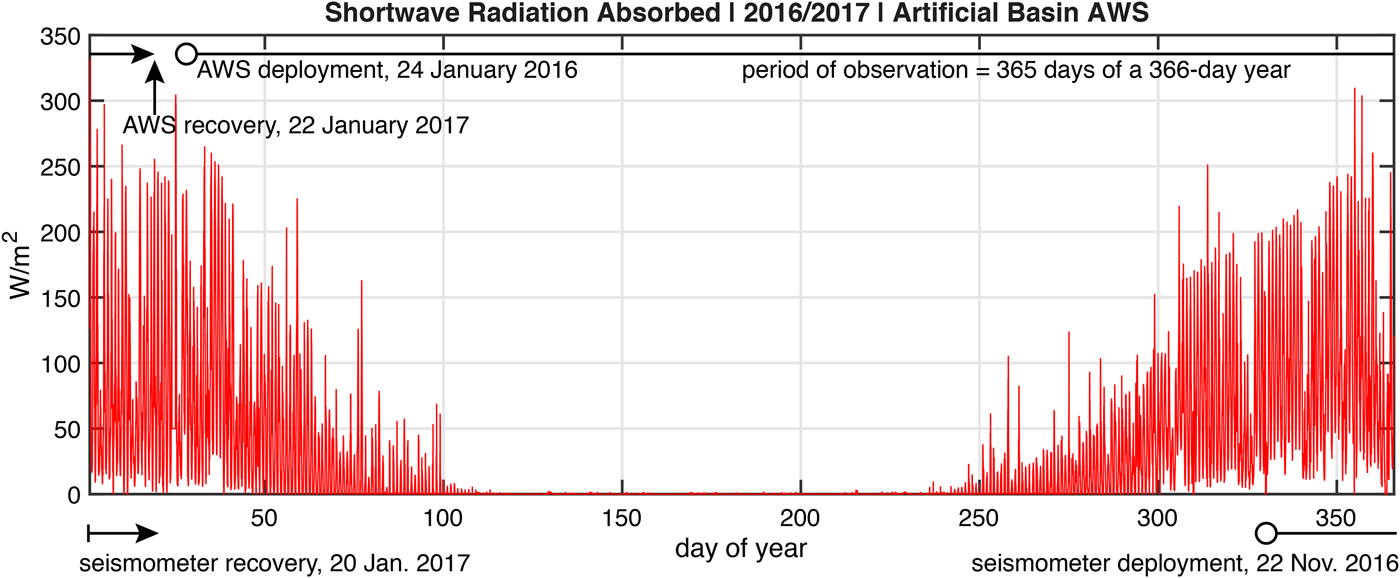
Fig. 10. Absorbed shortwave radiation (W m−2) measured 2 m above the surface at Artificial Basin using a 4-component radiometer. The longwave radiation was observed but not used in the parameterization of solar heating within the ice. This record has been re-expressed as a function of day-of-year for a perpetually repeating 366-day leap year to develop the annual record used as the solar forcing parameter s net for the thermal model. This annual forcing record was repeated during model spin-up to eradicate the effects of an arbitrary initial condition. Also shown are time-lines for AWS and seismometer operation relative to the derived annual record.
Model results
The thermal model was run for a period of 21 years, with each year's forcing being exactly the same time sequence of temperature and solar radiation as shown in Figs. 9 and 10. This model run was sufficient to stabilize T and Q so that they repeated the exact same time evolution in subsequent years. The initial condition was an arbitrary linear function between − 10°C at the surface and − 1.9°C at the bottom.
Results of the model simulation are shown in Fig. 11. The model produces temperate, water-filled ice immediately below a frozen lid, that is maintained by heat loss to the atmosphere above. Notably, from mid-December through late January, the surface temperature is at 0°C, and the lid thickness is 0. The net-water thickness (ice equivalent), distributed in the ice/water mixture reaches a maximum of 161 cm. Our simple model does not allow this water to move horizontally, for example, to drain away via surface streams or through the ice-shelf base by moulins. The water remains in place and is thus available to supply latent heat to the ice column through the Austral winter period.
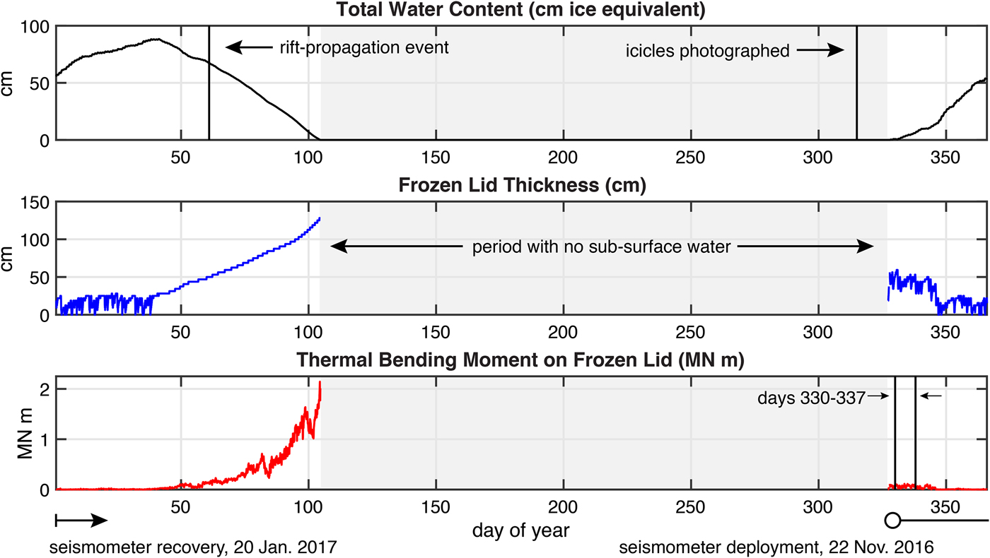
Fig. 11. Results of the baseline thermal model, total water in the ice column (top panel), thickness of frozen lid (middle panel), bending moment on frozen lid (bottom panel). Period when no subsurface (or surface) water exists on the ice shelf is indicated with gray shading. On day 61 (1 March 2016, vertical line in top panel) of the year, the rift on the McMIS that had previously terminated at Rift-Tip Lake (Fig. 1) propagated another 3 km. Inspection of the rift extension on approximately day 315 of the year ( ~11 November 2016) prior to the onset of surface or subsurface melting revealed that, over the Austral winter (probably immediately following the rifting event), subsurface water drained through the exposed walls of the rift, to form icicles seen in Fig. 12. The 8-day period shown in Figs 6, 7 and 13 is indicated on the bottom panel (i.e., days 330–337).
Although there are no direct observations to verify the model results given for the presence of subsurface meltwater, there is indirect evidence available from Banwell and others (Reference Banwell2017). They observed a rift propagation event occurring on 1 March 2016 (day 61 of the year) by satellite, and later went to inspect the newly extended rift on 10 November 2016 (day 315 of 2016), which was prior to the onset of the melt season following the rifting event (see timings of rift event and inspection indicated in Fig. 11). As shown in Fig. 12, icicles were found protruding from the rift walls just below the surface of the ice shelf on 10 November. Given that the rift walls were made on day 61 of the year, during the part of the year when the surface air temperature was falling, it is likely that these icicles represent residual subsurface water that leaked out of the rift immediately after its formation. The top panel of Fig. 11 shows that the total water content of the ice column was still above ~ 60 cm, and the middle panel of Fig. 11 shows that the subsurface water was covered by ~30 cm of frozen ice. These results are consistent with what is seen in the photograph of the rift walls shown in Fig. 12.
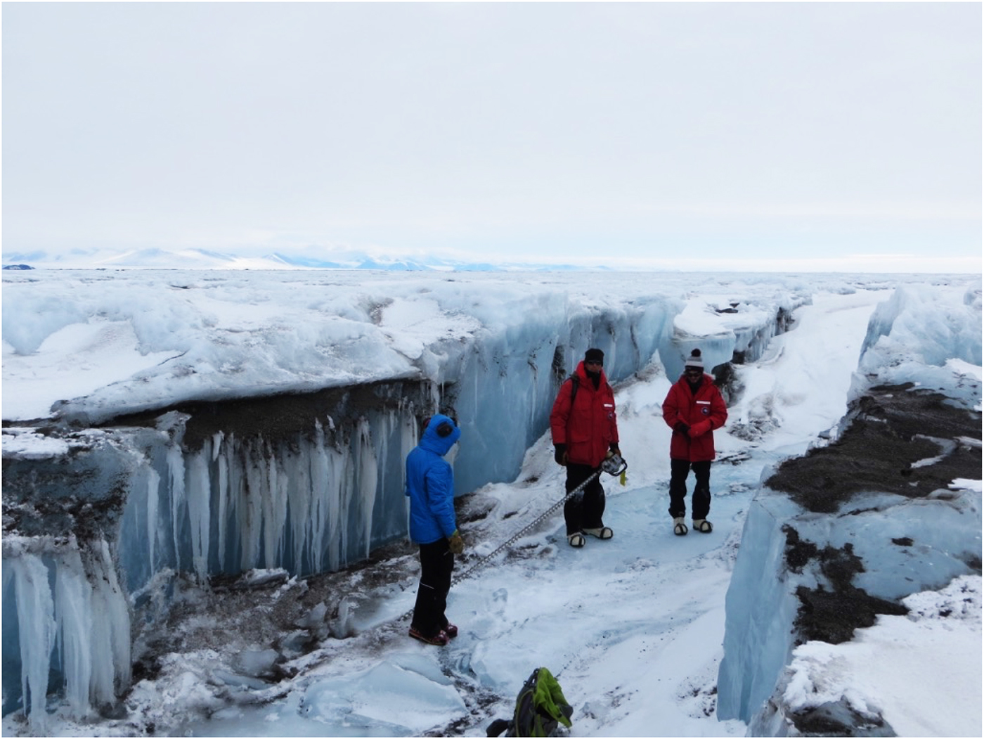
Fig. 12. Icicles protruding from subsurface layer along walls of a recently propagated rift (opening on 1 March 2016, see Banwell and others (Reference Banwell2017)). This photograph was taken on 10 November 2016, which was before renewed surface or subsurface melting on the ice shelf, immediately after the ensuing winter. We conclude that the most likely time for the icicles to have developed was immediately after the splitting of the ice shelf to form the rift walls on 1 March 2016. This was at a time when surface temperatures would have prohibited melting, hence the source of the water must have been subsurface residual from the preceding December/January period.
Thermal bending moment on frozen lid
The ‘frozen lid’ produced by the model is taken to be the cold ice layer with zero water content (Q = 0) that overlies a layer of temperate ice that contains water within its inter-grain space (Q > 0). If there is no temperate/slushy ice below the frozen lid, the frozen lid is assumed not to exist. The frozen lid first appears in the melt season around mid November (~ day 320) as a thin, ~ 0.5-m thick, superimposed ice cover that fluctuates in thickness until early February (~ day 40, Fig. 11). After about day 40, the lid monotonically thickens to ~125 cm as the subsurface water slowly freezes with the end of the austral summer melt season. The lid ceases to exist once the subsurface layer of temperate/slushy ice disappears around day 100 (9 April).
To pursue the hypothesis that the seismicity of the wet station is associated with thermal fracture, we compute the thermal bending moment per meter width of the frozen lid, M T (N m)/m, using the expression developed by Baz̆ant (1992; Eqn 5):
 $$ M_T(t) = {\displaystyle{E} \over {1 - \nu}} \alpha \Delta T(t) h_{{\rm lid}}(t)^2 I_T $$
where E = 5 GPa is the Young's modulus for ice, ν = 1/3 is the Poisson ratio for ice, α = 50 × 10−6 K−1 is the thermal expansion coefficient, h lid(t) is the frozen lid thickness (m), I T = 1/12 is a nondimensional shape function, and ΔT is the temperature drop between the lower side of the frozen lid, where T = 0, and the ice-shelf surface where T = T(z s, t) is expressed as a model boundary condition. The formula expressed in Eqn (5) is for a 2-D plate where all bending is confined to 1 dimension. The result of the baseline simulation is shown in the bottom panel of Fig. 11.
The evolution of the bending moment M T(t) over the melt season essentially mimics the frozen lid thickness h lid(t), due to its dependence on the square of the lid thickness (Eqn 5). What is most notable in the bending moment's evolution is the fact that it varies on a diurnal timescale, and can be compared with the seismicity for the period of 25 November--2 December (days 330–337), which is the time when the diurnal pulsation of seismicity contains the conspicuous ‘missing day's cycle’. A close-up of the baseline model results for 25 November--2 December (days 330–337) is shown in Fig. 13. The seismicity is plotted as a function of dM t/dt using the data and model results for this same period in Fig. 14. Notable in the comparison is that seismicity tracks increases of bending moment. This correspondence explains the conspicuous lack of seismicity on 30 November because the bending moment on that day rarely increases (except for a few short windows on the order of a few minutes). We conclude that the bending moment on a frozen lid produced by the thermal model constitutes a plausible explanation for the cause of the seismicity cycle seen in our data.
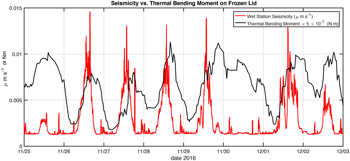
Fig. 13. Comparison of thermal bending moment on the simulated frozen lid, M T(t), with the standard deviation of seismicity for November 25--2 December 2016. Seismicity tends to correlate with periods of sustained daily increase of thermal bending moment. When the bending moment is constant, falling, such as is conspicuous on 30 November, or undergoing short-time-period changes, there is little-associated seismicity.

Fig. 14. Seismicity as a function of d/dtM T. Seismicity preferentially occurs when d/dtM T.
Reduction of diurnal seismicity during late December
Having used the 8-day window of observations from 25 November through the end of 2 December to develop a hypothesis for the cause of diurnal seismicity, we now examine the entire seismicity record (22 November 2016--14 January 2017) at the wet station to see if the hypothesis successfully predicts the seismicity over a longer time window. (While our seismometer deployment ran through to 20 January 2017, we discard the window from 15 January onward because of hydroacoustic noise in the seismic data associated with icebreaker and ship operations in McMurdo Sound). As shown in Fig. 15, the magnitude of the thermal bending moment on the frozen lid from 11 December 2016 to 14 January 2017 is much less than that before 11 December. This reduction in magnitude is seen to correspond with the elimination of the diurnal pulsations of seismicity, with the exception of a few isolated days. (Notable days in which the diurnal seismicity returned, ~19 December 2016 and 2 January 2017, were during periods when the weather was relatively cold.) This elimination corresponds with the time when the thickness of the frozen lid was generally zero in the model run (Fig. 11). The zero thickness was, in turn, due to the continued warming of the surface as the melt-season progressed. We regard the correspondence between the seismicity and thermal bending moment as further confirmation that periods of increasing bending moment are what cause the diurnal pulsations of seismicity.
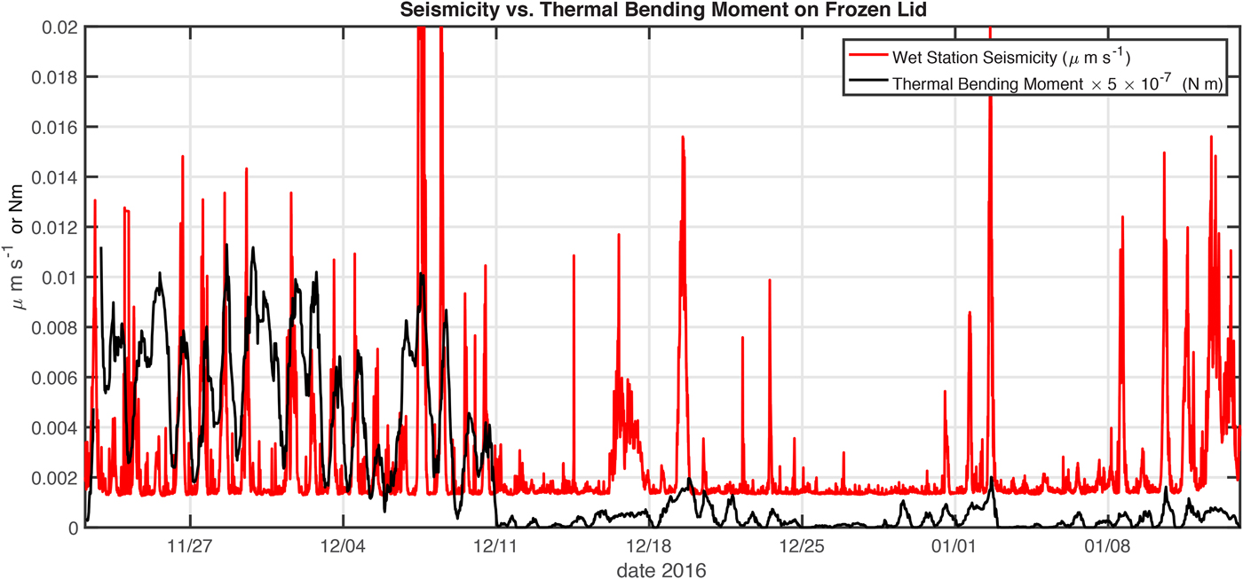
Fig. 15. Comparison of thermal bending moment on the simulated frozen lid, M T(t), with the standard deviation of seismicity at the wet station for 22 November 2016--14 January 2017. Diurnal seismicity pulses are absent during the time periods (e.g. starting on 11 December) when the thermal bending moment on the simulated frozen lid became very small or zero. The seismicity is not shown from 15 to 20 January because it was dominated by icebreaker and ship hydroacoustic noise from McMurdo Sound.
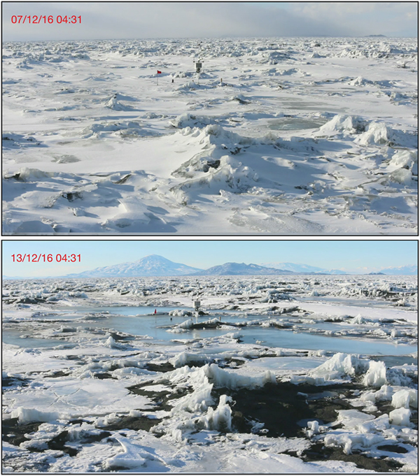
Our automated camera system (Fig. 1, Table 1) produced a record of surface conditions at Rift Tip Lake (Fig. 16). Figure 16 shows conditions on 7 December and 13 December, 2016, the 2 days that bracket the period of transition from robust diurnal seismicity to a complete absence of diurnal seismicity. The main difference visible in the two images is the replacement of a frozen surface with ice-free meltwater. This confirms that the frozen lid disappeared at roughly the time predicted by the model, and that this accounts for the fact that diurnal seismicity only happened sporadically after 13 December.

Fig. 16. Automatic camera photographs from 7 (top panel) to 13 (lower panel) December taken at 4:31 local time (UTC + 13). View is of a portion of Rift Tip Lake taken toward the South (Mount Discovery in the background) with an AWS in the middle ground. Conditions shown here are similar to those at the wet station. Prior to 13 December, and most strongly on 7 December, diurnally pulsed seismicity was observed 3 km to the West at the wet station. As the top picture confirms, this was during a period of time when the surface was covered by a frozen lid. After 12 December, the diurnal pulses of seismicity disappeared for days at a time. As the bottom picture shows, this corresponds to when the frozen lid had been melted through.
Dependence of model results on assumptions
We return to the question of how the comparison between diurnal seismicity and model-derived thermal bending moments on a frozen lid depends on the assumed T off = +1°C and s enh = 1.5. In model sensitivity simulations, we evaluated the two cases: (a) T off = +1°C and s enh = 1.0, and (b) T off = 0°C and s enh = 1.5. In case (a), a frozen lid covering subsurface water did not develop until day 333 corresponding to 28 November 2016, so the comparison between bending moment on the lid and seismicity was unsatisfactory. In case (b), without an offset warming, the period of time from 25 November through 3 December 2016, did not have a continuously present frozen lid, and, as with case (a), the comparison between the model-derived thermal bending moment and the observed seismicity was unsatisfactory. We conclude that, while our model and its forcing have been simplified to the utmost, its results are satisfactory for the simple purpose of identifying the cause of the diurnal seismicity.
DIURNAL SEISMICITY WAVEFORMS
To characterize the events of the diurnal seismicity cycle in terms of seismic phases is challenging because we have only one seismograph observing them. We examined a large number of individual events selected randomly throughout the window of observation and found that a few general descriptive comments can be made about the waveforms and phases comprising the vast catalog of events observed. Our comments must necessarily be viewed as preliminary until further study can acquire data from more than one seismograph.
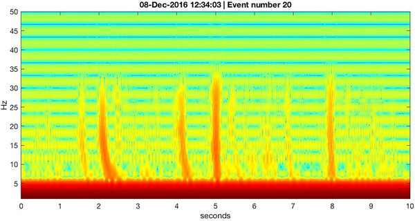
In Fig. 17, we show the spectrogram for a 10-second interval surrounding the 20th most prominent event (in terms of vertical ground motion) observed on 8 December 2016 at ~12:34 UTC. At 5 s in the spectrogram's horizontal axis, the 20th event is seen to be a sharply defined vertical swath of energy that is greatest in the 100--250 Hz frequency band, but which extends down to 1 Hz (the lower bound of sensitivity for the L28 geophone sensor, which was recording at 500 sps). This event's energy is consistent with a body wave propagating to the seismometer site from a nearby location.
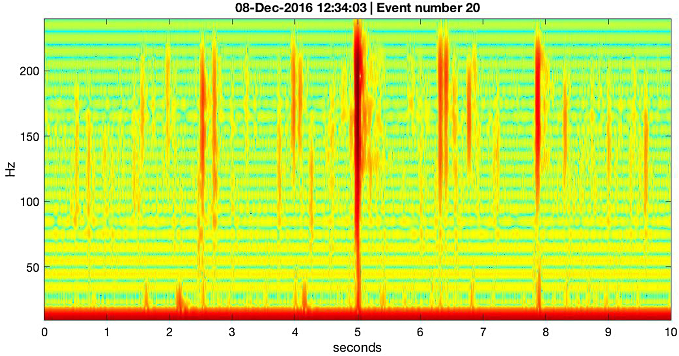
Fig. 17. Spectrogram of vertical ground motion (log velocity squared, relative color scale) observed with the wet station L28 geophone on 8 December 2016, during a prominent part of the diurnal seismicity cycle. The 20th most prominent amplitude event (event 20, out of > 1.6 × 10⁵ events detected on that day) is shown along with about 25 other small events. Event 20 shows energy distributed across all frequencies, consistent with an undispersed body wave propagating from a source location near the seismometer. The other events all exhibit a low-frequency cutoff that appears to range between ~ 25 and ~ 100 Hz. Below about 30 Hz, there are other signals, detailed in Fig. 18. Horizontal striping is likely an artifact of the MatLab routine (spectrogram()) used to make the spectrogram.
In the 5-second windows before and after the 20th event in Fig. 17, there are numerous smaller events (their ranking among the ~ 150 000 events observed during 8 December 2016 was determined but not of interest). These events show a curious low-frequency cutoff somewhere between 25 and 100 Hz (depending on event), and there are also discrete bands of energy at the low-frequency portion of the spectrogram, below ~30 Hz, which have an apparent high-frequency cutoff. We speculate that the low-frequency cutoff is likely due to the vertical arrangement of ice over water over solid earth rendering the water column a ‘slow’ layer sandwiched between two ‘fast’ layers in terms of body-wave phase velocity (MacAyeal and others, Reference MacAyeal, Sergienko and Banwell2015a,Reference MacAyeal, Wang and Okalb). This arrangement is analogous to the ‘SOFAR’ sound channel in the ocean (Ewing and Worzel, Reference Ewing and Worzel1948). The events that show the low-frequency cutoff in Fig. 17 are typical of the 10s of thousands of events of moderate to small magnitude, and this suggests that they are propagating as hydroacoustic phases from event sources distant on the order of hundreds of meters from the seismometer. The cutoff frequency, f cut, is related to the vertical thickness of the water layer,
 $$ f_{{\rm cut}} = {\displaystyle{c_{\rm s}} \over {d}} $$
where c s ≈ 1500 ms−1 is the speed of sound in seawater near 0°C, and d is the water-column thickness. This relation, and the 25–100 Hz cutoff frequency range observed in the data suggest that d ranges from ~ 15 to ~ 60 m, which is consistent with the bathymetry and ice thickness of the McMurdo Sound and McMIS, respectively.
At low frequency, below 30 Hz, the spectrogram in Fig. 17 displays signals that appear related to the high-frequency events, but which are restricted to frequencies below 30 Hz. A spectrogram of the low-pass filtered vertical ground motion (< 30 Hz) shown in Fig. 18 reveals that the signals tend to be reverse dispersed, with higher frequency components arriving before low-frequency ones. This is also evident in the seismogram of the signals, as displayed in Fig. 19. Phases displaying reverse dispersion are a prominent component of floating ice-sheet seismology, and are observed commonly in lake ice, sea ice and ice shelves (e.g. Ewing and Crary, Reference Ewing and Crary1934; Press and Ewing, Reference Press and Ewing1951; Hunkins, Reference Hunkins1960; Hatherton and Evison, Reference Hatherton and Evison1962; Xie and Farmer, Reference Xie and Farmer1994; Dudko, Reference Dudko1999, and references therein). A parsimonious explanation of the reverse-dispersed phases seen in the diurnal seismicity cycle is that they are generated when the superimposed ice lid imparts a vertical impulse to the ice-shelf immediately below as it undergoes thermal fracture (e.g. Yang and Yates, Reference Yang and Yates1995).

Fig. 18. Spectrogram of low-pass filtered (30 Hz) vertical ground motion (log velocity squared, relative color scale) observed with the wet station L28 geophone on 8 December 2016, during a prominent part of the diurnal seismicity cycle. Events near 2 and 4 s exhibit reverse dispersion, where high-frequency energy arrives before low-frequency energy. Waveforms of the low-pass filtered vertical ground motion shown here are shown in the seismogram of Fig. 19. Horizontal striping is likely an artifact of the MatLab routine (spectrogram()) used to make the spectrogram.

Fig. 19. Seismogram of the low-pass filtered (30 Hz) vertical ground velocity (μm s−1) at the wet station associated with the spectrogram of Fig. 18. Events near 12:34:01 and 12:34:03 clearly display reverse dispersion.
DIURNAL SEISMICITY STATISTICS
A notable aspect of the diurnal seismicity cycle is the fact that it involves very large numbers of relatively small events. To provide some sense of what number of events are involved and how their amplitudes are distributed, we attempted to count them. Following Carmichael and others (Reference Carmichael, Pettit, Hoffman, Fountain and Hallet2012, 2017), we experimented with using a short-term/long-term signal variance detector to determine the onset and amplitude of individual events. Difficulty in the implementation of this detector due to the variability of intra- and inter-event timescales led us to use the MatLab™ function findpeaks() as a means of identifying and measuring the amplitude of single events. After experimentation with the parameters that characterize the event detection algorithm findpeaks(), we selected a minimum peak threshold (1 μm s−1 in the vertical ground motion) and a minimum peak time separation (0.1 s) to exclude multiple peak detections within a single apparent event. This approach thus means that multiple events which occur within a time window of 0.1 s or less will contribute one detection (the first one to occur) to the event statistics. Furthermore, the detection algorithm does not exclude noise features that are unrelated to the diurnal seismicity, and it is difficult to assess the uncertainty in the event statistics that result. Assuming the noise features to be of uniform amplitude during the entire day, the minimum peak threshold (1 μm s−1) in the vertical ground motion chosen for the detection algorithm was higher than the noise features observed during quiescent periods of the diurnal cycle.
Using the 500-Hz vertical ground velocity channel of one of the two short-period instruments deployed at the wet station (the other instrument did not stay level through the observation period), we identified > 2 × 10⁶ events during a 53-day window when the presence or absence of a diurnal cycle could be attributed to natural causes, and not to interference from anthropogenic icebreaker and ship noise. The 500-Hz vertical ground velocity signal was first high-pass filtered with 100 Hz as the pass frequency to emphasize the dominant frequency band of the majority of events determined from Fig. 17. A summary of the event timing and their amplitude is shown in Fig. 20.
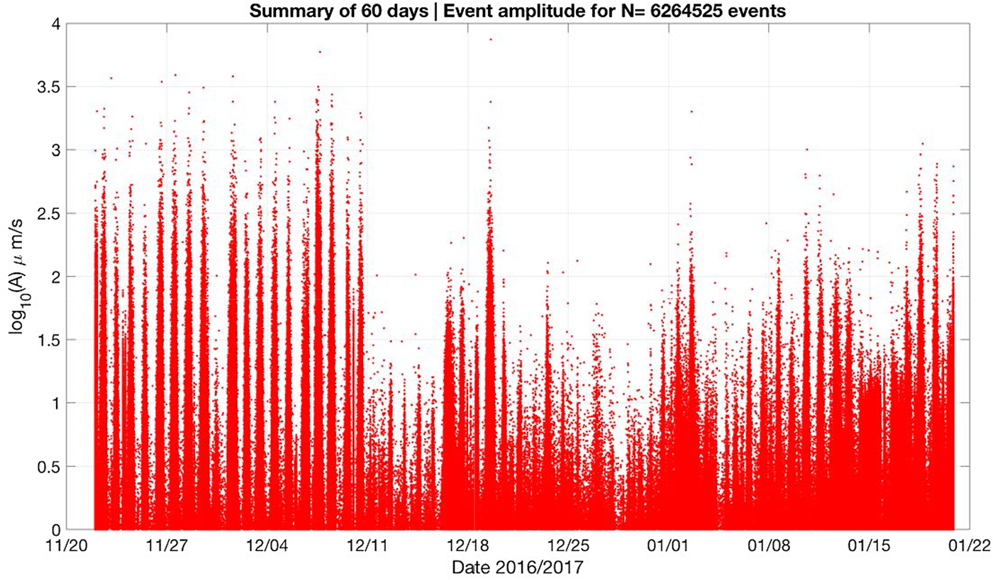
Fig. 20. Individual seismic events detected from 100 Hz high-pass filtered vertical ground motion at the wet station during a 53-day period (23 November 2016--14 January 2017) used to compute event amplitude distribution N. Data from 14 to 20 January 2017 were excluded due to the presence of anthropogenic tremor from icebreaker and ship activity in McMurdo Sound. The event detection algorithm was simple, involving peak detection (findpeaks() from MATLAB) with a specified low-amplitude cutoff and time window following a given event detection during which no further events would be detected. The algorithm likely leads to a bias in detecting noise features at low amplitudes that are unrelated to the diurnal seismicity cycle.
Using the event detection algorithm described above, we investigated how the number of events varied with event-amplitude measured at the seismometer site. This approach constitutes a variant to classical frequency-size investigations, which have been carried out routinely since Gutenberg and Richter (Reference Gutenberg and Richter1954) noted that, in any population of earthquakes, the logarithm (base 10) of the number N(M) of events with magnitude at least equal to M varies as
 $$ \log_{10} N(M) = C - b \ M $$
Because of the mathematical properties of the logarithm function, Eqn (7) also applies with the same b-value to the opposite of its derivative n(M) = −dN/dM, i.e., to the number of events falling into a magnitude bin of constant width centered on a magnitude value M:
 $$ \log_{10} n(M) = c - b \ M $$
In practice, the ‘Gutenberg and Richter law’, hereafter ‘GR’, applies remarkably well with b ≈ 1 in Eqns (7) or (8) to most populations of shallow earthquakes. This property was later justified based on scaling laws, for fault zones with a fractal dimension of 2 (Rundle, Reference Rundle1989). A departure from GR, and, in particular, a b-value >1, illustrates a different mechanism of seismogenesis, for example, involving a 3-D medium as opposed to a fault, as found for certain classes of deep earthquakes (Okal and Kirby, Reference Okal and Kirby1995), or in the highly brecciated material where a large number of fractures hinders the growth of the source for large seismic events (e.g. McNutt, Reference McNutt, Lee, Kanamori, Jennings and Kisslinger2002). For example, a high b-value is generally a proxy for volcanic earthquakes releasing the stress transferred into the volcanic edifice by the ascent of magma (e.g. Yuan and others, Reference Yuan, McNutt and Harlow1984).
In the present study, we can only quantify the events through their recorded amplitude A, rather than through a magnitude M, which would have to be obtained by applying a distance correction to log 10A; with only one recording station, we cannot infer epicentral distance and carry out such a correction. Faced with similar circumstances, many scientists have simply fit a GR law to the distribution of recorded amplitudes (using a logarithmic scale)
 $$ \log_{10} n(M) = C_1 - b_1 \ \log_{10} A $$
and interpreted their results under the assumption that the observed opposite slope, b 1, is indeed the physical b-value of the original distribution of seismic sources; this was the case, for example, of the first studies, using a single ocean-bottom seismometer, of the micro-seismicity associated with earthquakes along oceanic rifts (Francis and others, Reference Francis, Porter and McGrath1977). This assumption would obviously be correct if all events were at the same distance from the receiver, and hence their amplitudes identically affected by propagation. We show in Appendix A that it does indeed hold (at least for the smaller earthquakes in the dataset considered) for a number of geometries where epicentral distance varies, but the spatial density of sources is constant.
In this context, our observable ‘amplitude’ A recorded on the short-period seismometer can be regarded as ground velocity, measured in μm/s−1 (L28, Table 1). We proceed to evaluate the population of events as a function of amplitude by binning the data into intervals αi ≤ A ≤ αi+1, with  $\alpha _i = \alpha _0 + i \ \Delta \alpha $, and define a cumulative population N as a function of amplitude A as the number of events with an amplitude at least equal to A; note that this definition is independent of the details of the binning procedure. We then use log 10A as a substitute for observed magnitude M and study the distribution of log 10N as a function of M.
Using the entire 53-day observation window to compute N, the result is shown in Fig. 21. The main feature of this distribution is the increasing negative slope of the distribution with increasing log 10(A). While it is tempting to compare the shape of this distribution, with the slope corresponding to minus the ‘b-value’ of the Gutenberg--Richter distribution for earthquakes, this should not be done, because log 10(A), the argument of N, is not corrected for distance, as is the case for M, earthquake magnitude.
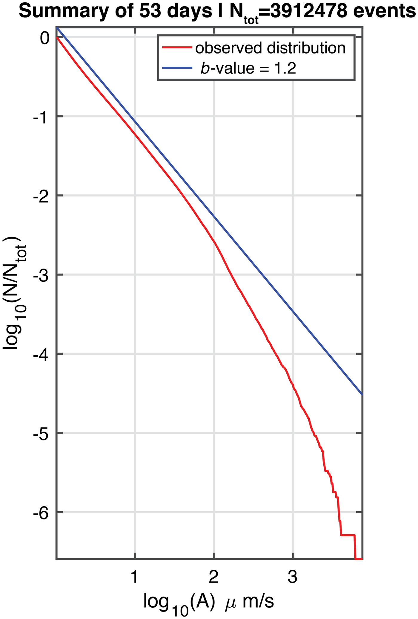
Fig. 21. Distribution of N for high-frequency events (>100 Hz) observed at the wet station during the 53-day window (23 November 2016--14 January 2017) when diurnal seismicity was prominent. The observations from 14 to 20 January were excluded due to the presence of ship tremor.
The population N(A) shown in Fig. 21 is characterized by a GR distribution with a slope b 1 ≈ 1.2 for low amplitudes (A < 60 μm/s−1), beyond which an elbow is present and b 1 increases significantly, to values of the order of 3. As discussed in the Appendix, the low-magnitude end of the population implies a similar GR distribution with an intrinsic b 0 = 1.2 for the events recorded. The experiments reported in Appendix A would suggest that the position of the elbow is related to the maximum (true) magnitude m max of the events, to the dominant frequency of the wavetrains (~100 Hz), to the unknown epicentral distance, and to the seemingly unknown anelastic attenuation along the path to the station.
Irrespective of the fractal dimension of the seismogenic material, many factors can affect the b-value of a population of earthquakes. In very general terms, a b-value slightly larger than 1 could be expected in a fractured medium (Mogi, Reference Mogi1962) where faults will have difficulty growing coherently to large dimensions, and for low stresses, as b-values have been found to decrease significantly with increasing ambient stress (Scholz, Reference Scholz1968). Such conditions seem legitimate in the particular environment of the ice shelf. While these preliminary remarks are encouraging, it would be futile to attempt deeper interpretation in the absence of an adequate knowledge of fundamental parameters such as epicentral distances.
A remarkable property of the low-frequency signals described in the previous section (see Figs 18 and 19) is that they obey different population statistics from those shown for the high-frequency signals. (Restricting the event counting routine to low-frequency signals was accomplished by applying the detection algorithm to a low-pass filtered time series.) As shown on Fig. 22, they exhibit a value b 1 ≈ 3 much higher than their high-frequency counterparts, with a much less pronounced, if at all defined, elbow. Their lower dominant frequencies would argue for longer wavelengths, and hence a generally larger source, even though the range of their ground velocities recorded at the receiver is not significantly different from that for the high-frequency events. In this context, we recall that the scaling of strong motion ground velocities (or a fortiori accelerations) with earthquake size in the near field can deviate from simple power laws predicted by source similitude arguments (Anderson and Lei, Reference Anderson and Lei1994; Abrahamson and Silva, Reference Abrahamson and Silva1997). In the general framework of a highly fractured source medium, we would certainly expect a decrease of the population of large events, and thus an increase in b-values at the source. As for the weakening or absence of the elbow, it is probably a direct consequence of the higher b-values, as evidenced on Fig. 23: when fewer large events are present the effect of the upper bound m max on the undersampling of large observed amplitudes will be weaker.

Fig. 22. Distribution of N for low-frequency (< 30 Hz), reverse-dispersed events recorded during a 53-day period (23 November 2016--14 January 2017) when diurnal seismicity was prominent. The observations from 14 to 20 January were excluded due to the presence of ship tremor.
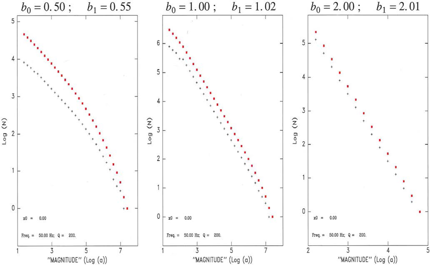
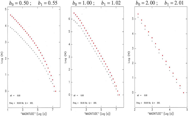
Fig. 23. Populations of observed amplitudes interpreted as ‘magnitudes M’ for a dataset of earthquake sources with magnitudes m obeying a GR law with an initial b-value of 0.5 (Left), 1 (Center) and 2 (Right). The earthquakes are distributed with a constant density μ along a linear segment of length L = 10 km, with the receiver located at one end of the segment. The plus symbols are the populations of the individual magnitude bins, and the red dots are the cumulative values. The apparent b-values, b 1, are obtained by linearly regressing the cumulative populations.
DISCUSSION AND CONCLUSION
One signal revealed by our modest seismometer deployment was not previously observed on an ice shelf and it was only observed in the ‘wet’ area of the McMIS (Fig. 1). It consisted of a pervasive diurnal cycle of seismicity, featuring hundreds of thousands of very small icequakes each day, clustered in time when temperatures were falling. At times of the day when surface temperatures were stable or rising, or at times when there was pervasive standing water on the ice shelf, virtually no seismicity was observed (at frequencies > 1 Hz). The diurnal seismicity cycle was only observed at the wet station and is thus presumed to be caused by processes associated with surface melt/freeze cycles.
The diurnal seismicity cycle had sufficient day-to-day variability to allow its cause to be deduced. For example, we were able to rule out the tidal-flexure process seen elsewhere on ice shelves, most notably at a dry ice-shelf site near the grounding line of Kamb Ice Stream (Hulbe and others, Reference Hulbe2016), because days when the seismicity cycle was missing did not show unusually small tidal displacement. (We do not rule out, however, that tidal flexure and other movements do not drive other, smaller-amplitude periods of seismicity on the McMIS. We simply note that tide was not responsible for the conspicuous large diurnal pulsation of interest here.) The physical process that most readily correlates with the seismicity cycle and its variation from day to day was found to be thermally induced bending and fracture of a ‘frozen lid’ that overlies a near-surface partial melt zone.
To test this mechanism, we constructed a simple, idealized thermal model of the ice shelf and simulated the development of subsurface partial melt layers. When forced with AWS-derived weather conditions, the model produced volumes of meltwater, frozen lid thicknesses and thermal bending moments that were consistent with the observed variation in seismicity.
Two types of seismic waves are prominent in our observations. At high frequency, most events are hydroacoustic phases exhibiting a low-frequency cutoff (25–100 Hz). This cutoff is likely induced by the seawater layer between the ice shelf and the seabed which has low sound speed relative to the layers above and below. At low frequency, most events are probably flexural-gravity waves that have a high-frequency cutoff (30 Hz), and that display reverse-dispersion, with high-frequency arriving before low-frequency. These two types of seismic waves follow different population statistics; the high-frequency events feature a Gutenberg--Richter distribution with an intrinsic b-value of 1.2, previously observed in fractured media rupturing at low ambient stress, as is consistent with an ice lid superimposed on a subsurface slush layer. The low-frequency events, whose larger wavelengths would advocate larger source dimensions, expectedly feature a higher b-value, of the order of 3.
We speculate that thermally regulated seismicity may exist on all ice shelves that undergo surface melting and freezing, especially those that have lost their protective, insulating firn layer. We agree, therefore, with previous studies (e.g. Chaput and others, Reference Chaput2018; Podolskiy and Others, Reference Podolskiy, Fujita, Sunako, Tsushima and Kayastha2018) suggesting that seismological methods may be a practical means of monitoring glacier surface conditions over a wide area and through long periods of time. In addition, we note that some seismic signals on ice shelves, such as those associated with surface lake induced hydrofracture, may be masked by seismicity associated with near-surface thermal forcing. The agreement between the numerical model of thermal forcing and seismicity seen in our data suggests it may be possible to use local weather data to separate seismic signals associated with thermal forcing from those due to other phenomena.
ACKNOWLEDGEMENTS
We thank the US Antarctic Program, UNAVCO and IRIS/PASSCAL, especially Phillip Chung and Pnina Miller, who have made our study, particularly our presence in the field, possible. We also acknowledge help by Mike Cloutier and the PGC. This work was supported by US National Science Foundation grant PLR-1443126. Seismic data are archived for public distribution at the IRIS Data Management Center (DMC), and is identified by network ID 9G. AWS and GPS data are archived at the US Antarctic Program Data Center (USAP-DC), and are identified by digital object identifier (doi) numbers 10.15784/601106 and 10.15784/601107. AWS data are additionally archived at the University of Wisconsin's Antarctic Meteorological Research Center (AMRC). AFB acknowledges support from a Leverhulme/Newton Trust Early Career Fellowship. GJM acknowledges support from a NASA Earth and Space Science Fellowship (NNX15AN44H). We thank Brad Lipovsky for discussion and valuable suggestions on the analysis presented here. The two anonymous referees and scientific editor who reviewed this manuscript provided extremely good comments and criticism.
AUTHOR CONTRIBUTION
DRM, EAO and JL conducted the seismological data analysis. EAO conducted the theoretical analysis presented in the Appendix. AFB, ICW, BG and GJM deployed and recovered the seismographs in the field. All authors were involved in conceiving and writing the manuscript.
APPENDIX A. GR STATISTICS FOR A POPULATION OF EARTHQUAKES AT UNKNOWN DISTANCES
We consider here the effect of propagation over an unknown (and assumed variable) distance x on the distribution of observed amplitudes, and hence of observed b-values. In very general terms, the decay of a seismic wave with distance has two components, one purely elastic, the other anelastic. The elastic effect is known as geometrical spreading and depends on the nature of the wave: a body wave propagating in a conceptually unlimited, 3-D space will see its amplitude decay as 1/x while a wave propagating in a vertically restricted waveguide (including interface waves such as Rayleigh waves) will feature a  $1/\sqrt {x}$ dependence. At very short distances, comparable to the wavelength of the wave, the near field terms of body waves, which scale as 1/x 2, would become prominent. In addition, anelastic attenuation will dampen the amplitude of a seismic wave as
 $$A(x) = A_{{\rm init}}\,e^{-\gamma x}; \quad {\rm with} \quad \gamma = \displaystyle{{\omega} \over {2 Q V}}$$
where ω is the dominant angular frequency of the wave, V its [group] velocity and Q the quality factor of the medium. Because of the exponential nature of Eqn (A1), anelastic attenuation eventually becomes dominant at large distances.
We consider the problem of a population of earthquakes distributed with a parameter b 0, and observed at a variable distance x, the question being ‘Does the population of observed amplitudes satisfy a GR law and, if so, what is the relationship between the observed b 1 at distance x and the original b 0?’
We start with the simple model of a line source where seismicity is distributed along a 1-D axis, with a constant density of source per unit length, μ. The amplitude A observed at some distance x from an event originating with a magnitude m will result from the combination of m and of the attenuation suffered along the path. The combination of geometrical spreading and anelastic attenuation can be represented by a function Φ(x);
 $$\Phi(x) = \Phi_{0} \displaystyle{{\exp {( - \gamma x)}} \over {x}} \quad {\rm or} \quad \Phi(x) = \Phi_0 \displaystyle{{\exp{( - \gamma x)}} \over {\sqrt{x}}}$$
depending on the nature of the wave (body or guided), which controls geometrical spreading. The observed amplitude is then
 $$ A(x,m) = A_0 10^m \cdot \Phi(x) $$
and the apparent ‘magnitude’ M, defined as
 $$ M = \log_{10} \left ( A / A_1 \right ) $$
(where A 0 and A 1 are constants) will simply be
 $$ M = m + \log_{10} \Phi(x) + M_2 $$
with M 2 being yet another constant.
For any given x, the number of events originating between x and x + dx and observed with an apparent magnitude > M will be the number dN of earthquakes with an initial magnitude
 $$ m \gt M - \log_{10} \Phi(x) - M_2 $$
or
 $$ dN = \mu dx \cdot \displaystyle 10 ^{ C_0 - b_0 \left ( M - \log_{10}\Phi(x) - M_2 \right ) } $$
The total number N of such earthquakes is obtained by simply integrating Eqn (A7) over x. Assuming a simple geometry where the observation point is at the end of the line source of length L,
 $$ N(M) = \mu \int_0^L 10 ^{ C_0 - b_0 \left ( M - \log_{10}\Phi(x) - M_2 \right ) } \cdot {\rm d}x $$
 $$ = \mu 10^{ C_0 - b_0 \left ( M - M_2 \right ) } \cdot \int_0^L \left [ \Phi(x)\right ]^{b_0} \cdot {\rm d} x $$
which takes the form
 $$ N(M) = N_2 \cdot 10^{-b_0 M}; \quad \log_{10}N(M) = C_2 - b_0 M \ \ . $$
It is easily verified that a similar conclusion would be reached if the receiver is outside, or inside, the line source. Its physical interpretation is that, because distance-controlled attenuation is independent of original source size (magnitude m), it affects events of all sizes in the same way and does not perturb the relative distribution of earthquake sizes.
We verified this property by numerically building populations of earthquakes originally satisfying GR laws with various values of b 0, and applying full distance corrections including geometrical spreading. Fig. 23 shows results for a receiver located at the end of the line source (L = 10 km), a 1/x geometrical spreading law, a P-wave velocity in the ice of 3 km s−1, a dominant frequency of 50 Hz and a quality factor of 200; we tested three original b-values, b 0 = 0.5, 1 and 2, respectively. The apparent b-value, b 1, is computed by linearly regressing the cumulative distribution of observed magnitudes. It is clear that the lemma is verified for the small-magnitude portion of the dataset, but that the population of larger events becomes deficient when the magnitude is increased. This is an artifact of the necessity, in our computational exercise, to use an upper limit for the original magnitude m, since we cannot extend it to infinity. When reaching large values of M, the magnitudes m given by Eqn (A5) are undersampled, and we have verified that the domain where this effect becomes significant is a function of the imposed m max, of x, of the parameters defining Φ (e.g. ω and Q), and of the distribution of source size and hence b 0. In retrospect, this apparent limitation in our models is actually reproduced in real life, since the magnitude of the events observed on the ice is expected to be limited upwards by the coherence length over which rupture can develop inside the seismogenic medium.
However, it is important to keep in mind that the development of the elbows in Figs 23 to 25, and the subsequent increases in b 1 are rooted in the presence of a maximum source magnitude m max (which can be physical, as probably is the case for our icequake populations, or artificially imposed by the impossibility of reaching an infinite magnitude in our numerical models). It does not necessarily reflect a genuine change in scaling laws, as for example in the case of the distribution of seismic moments for shallow earthquakes, where an elbow is also observed when the growth of seismic sources is affected by the saturation of fault width at depth (e.g. Okal and Romanowicz, Reference Okal and Romanowicz1994, Fig. 1). In simple terms, an elbow in b 1 does not require one in b 0, if the population of sources is limited to a maximum magnitude m max, but keeps a constant b 0 below that value.
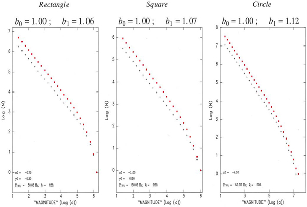
We further tested the robustness of our results with respect to a variation of the geometry of the parameters of the model, with representative examples given on Fig. 24, where we moved the receiver inside the line source (Left), used a much lower level of attenuation (Q = 1000 at f = 10 Hz; Center), or considered a guided wave with a geometrical spreading varying as  $1/\sqrt {x}$ (Right), with no significant effect on the main result, i.e., in all cases b 1 ≈ b 0. Finally, in Fig. 25, we explore different geometries, by replacing the line source with a 2-D seismogenic zone of rectangular (Left), square (Center), or circular (Right) shape; once again, we conclude that our results are robust, with b 1 essentially reproducing b 0, especially at low magnitudes.
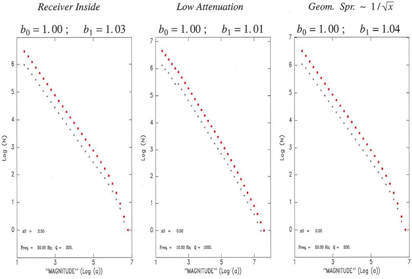
Fig. 24. Same as Fig. 23 for a receiver located inside the line source (Left); a significantly less attenuating medium (Q = 1000 at f = 10 Hz; Center); and a guided wave with geometrical spreading falling as  $1 / \sqrt {x}$ (Right). Note robustness of results.
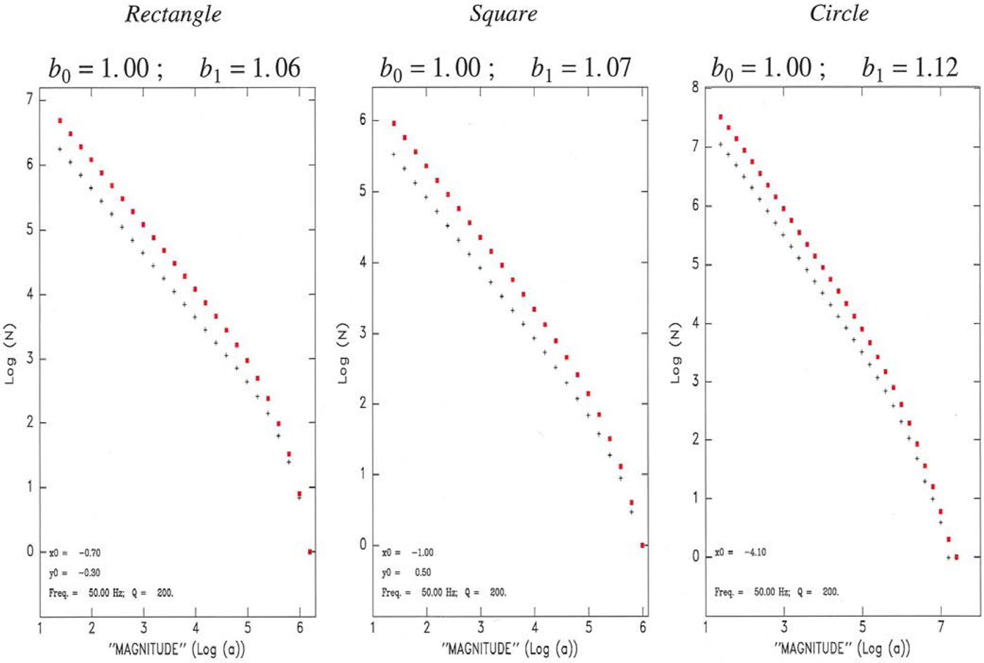
Fig. 25. Same as Fig. 23 for a receiver located outside a rectangular seismogenic zone (Left); outside a square seismogenic zone (Center); and inside a circular seismogenic zone (Right). Note robustness of results.


 Open access