


Introduction
A geographical pole of inaccessibility is generally defined as that point which is most distant from a coastline (Garcia-Castellanos & Lombardo, Reference Garcia-Castellanos and Lombardo2007; Stefansson, Reference Stefansson1920). The concept has been applied both to oceans (where it refers to the point farthest from land) and to islands and continents (where it becomes the point farthest from water). In the former sense, the Arctic Pole of Inaccessibility has recently been shown to lie at 85° 48’ N, 176° 09’ W (Rees, Headland, Scambos, & Haran, Reference Rees, Headland, Scambos and Haran2014), correcting an inexplicable but persistent error of over 200 km in its stated position.
The corresponding concept for the Antarctic uses the opposite sense of the definition, i.e. the point on the surface of the continent farthest from its “edge”. However, more than one definition of this edge is possible. In all cases, the edge represents the boundary on the map between two different surface types. The Scientific Committee on Antarctic Research’s Antarctic Digital Database (the SCAR ADD) defines coastlines with respect to land, ocean, ice shelves, ice tongues and ice rumples (ADD3.0, 2000), and these coastlines together form a set of topological polygons. Outside the outermost polygon lies the ocean, while inside the innermost polygon lies the “true” continent, shorn of any floating ice. These two extremes form the two accepted definitions of the “edge” of Antarctica, from which the Southern Pole of Inaccessibility (SPI) is found. They will be referred to here as the inner and outer coastlines.
Where is the SPI located? As with the Arctic Pole of Inaccessibility, there has been some uncertainty and confusion about this, and some variation in the accepted position over time. It seems probable that much of this variation can be attributed to errors of calculation or of transcription, rather than significant alteration of the geographical facts. A research station was established by the Soviet Union in December 1958 during the International Geophysical Year. The location (82° 06’ S, 54° 58’ E) was chosen to be close to the calculated position of the pole of inaccessibility, and this was the name given to the station: Полюс недоступности (Polyus Nedostupnosti) (Petrov, Reference Petrov1959). (Note that geographical locations are specified in the text with a precision of 1 min of arc, although some of the underlying data are given with greater precision than this.) Although the Soviet Union went to the trouble of erecting a bust of Lenin at the site, it was largely abandoned after only a couple of weeks of operation (Gan, Drewry, Allison, & Kotlyakov, Reference Gan, Drewry, Allison and Kotlyakov2016). However, it appears to have served as something of an authority for subsequent statements about the position of the SPI. In the terms defined in the previous paragraph, it corresponds approximately to the SPI of the inner coastline.
Subsequently stated locations of the “inner” SPI have been rather variable. Headland (1996: https://web.archive.org/web/20160528131216/http://www.spri.cam.ac.uk/resources/infosheets/23.html) placed it at 85° 50’ S, 65° 47’ E; the British Antarctic Survey was quoted as having located it at 82° 53’ S, 55° 04’ E (2005: https://web.archive.org/web/20160414194423/http://www.explorersweb.com/polar/news.php?id=1298), the International Polar Heritage Committee gave a position (2016: https://web.archive.org/web/20070929161454/http://www.polarheritage.com/index.cfm/Sitelist01up) of 83° 06’ S, 54° 58’ E, and the Atlas Obscura website (https://www.atlasobscura.com/articles/have-fun-trying-to-reach-the-poles-of-inaccessibility; retrieved 2020-11-12) confidently locates it, with a precision equivalent to around 1 cm, at 76° 19’ S, 49° 26’E. These locations are shown in Figure 1(b). Some are probably mistranscriptions of others, while the last mentioned is clearly though inexplicably incorrect. We have not found any statements of the position of the “outer” SPI before one attributed to BAS (2005: https://web.archive.org/web/20160414194423/http://www.explorersweb.com/polar/news.php?id=1298), which located it at 83° 51’ S, 65° 44’ E. Using a new method, Barnes (Reference Barnes2019) calculates an inner SPI of 77° 24’ S, 105° 23’ E and an outer SPI of 78° 16’ S, 103° 38’ E; subsequent analysis shows these values are incorrect because the data they are based on split the Antarctic continent into two large polygons, a mistake we do not make here. As noted by Rees et al. (Reference Rees, Headland, Scambos and Haran2014), verification of the location of a pole of inaccessibility requires the identification of the three points on the coastline from which it is maximally equidistant, which we refer to as tangent points (the concept is equivalent to that of “closest shoreline points” defined by Garcia-Castellanos and Lombardo (Reference Garcia-Castellanos and Lombardo2007)). All online statements about the location of the SPI that we have been able to find fail to include information about the location of these tangent points, which makes it difficult to assess them.
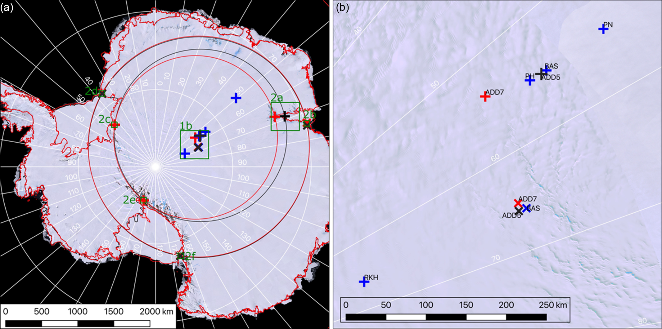
Fig. 1. (a) Map showing positions of SPI and tangent points, and circles centred on SPIs and passing through tangent points. Black symbols and lines refer to ADD5, red symbols and lines to ADD7.2 and blue symbols to other SPI positions reported in the literature. “+” = inner coast, “×” = outer coast. Ice sheets are labelled. (b) Enlargement of the central part of (a), identifying SPI positions excluding the outlier position reported by Atlas Obscura. PN = Polyus Nedostupnosti (Soviet IGY station), PH = Polar Heritage (2016), RKH = Headland (1996), BAS = British Antarctic Survey (2005: https://web.archive.org/web/20160414194423/http://www.explorersweb.com/polar/news.php?id=1298). Background: Centre-filled LIMA (Landsat Image Mosaic of Antarctica: Bindschadler et al. Reference Bindschadler, Vornberger, Fleming, Fox, Mullins, Binnie and Gorodetzky2008).
Another factor contributing to uncertainty in the location of the SPI is its dynamic nature. While no coastline can be said to be truly static, Antarctic coastlines, especially the outer coastline, are especially variable over time. Changing coastlines are likely to change the position of the SPI.
The aim of this paper is to determine an accurate current position for the SPI and to assess the rate at which it has moved during the present century. Fundamental reference data for the task are available from the SCAR ADD (Thomson & Cooper, Reference Thomson and Cooper1993). This has been updated several times since its original compilation in the 1990s, the updates reflecting both real changes in the location of coastlines and improvements in cartographic techniques. Comparing an older version of the ADD coastline with the current version is an appealing option to examine how change in the coastline has affected the position of the Pole of Inaccessibility, though the changes in technique need also to be borne in mind. Earlier Landsat data had very poor spatial positioning and relied on ground survey data for location, data that may not have existed in some areas and large areas were often obscured by cloud cover. A further difficulty occurs in the case of the inner coast defined by the ice grounding line. In earlier versions of the ADD, the grounding line was based on interpretation by glaciologists, based on features such as crevassed areas indicating a hinge zone, changes in slope (from shading on the images) and visible flow lines on the images. ADD 1 had a baseline dataset for this interpreted by hand onto film overlays from hard-copy images by an experienced Antarctic glaciologist from Landsat MSS images mosaicked together and then positioned as best as possible. This was an attempt to define what could be achieved from the available data in 1990. During the lifetime of the ADD, the grounding line has come to be defined from changes in velocity of the ice as it starts to float, using feature tracking in Landsat imagery and using radar interferometry (Bindschadler et al. Reference Bindschadler, Choi, Wichlacz, Bingham, Bohlander, Brunt and Young2011; Rignot, Mouginot, & Scheuchl, Reference Rignot, Mouginot and Scheuchl2011).
Datasets
The “present-day” locations of the SPI for both inner and outer coastlines were calculated using coastline data downloaded from the ADD v7.2 (https://www.add.scar.org/). These coastline data, revised within the last 10 years in the majority of regions, were downloaded as line-feature shapefiles. We also acquired data for ADD v5, the earliest version of the ADD for which suitable shapefiles were available.
ADD v7.2 defines several types for coastline which are composed to form polygons which delineate the Antarctic continent. We represent the inner coastline by composing the “rock coastline”, “rock against ice shelf”, “ice coastline” and “grounding line” coast types; we represent the outer coastline with the “ice coastline”, “ice shelf and front” and “rock coastline” types. For ADD v5, we use all coast types to represent the inner coastline and the 22010 (ice coastline), 22011 (rock coastline), 22020 (ice coastline), 22021 (rock coastline) and 22050 (ice shelf front) types to represent the outer coastline.
These data are archived on Zenodo (Barnes, Reference Barnes2021) and available via the SCAR ADD website.
Modern calculation of present-day positions and rates of change
To ensure the accuracy of our results, we performed two independent calculations.
The first calculation is based on an iterative search procedure described by Garcia-Castellanos and Lombardo (Reference Garcia-Castellanos and Lombardo2007). The procedure starts by taking as input a box large enough that it surely contains the SPI. We generate this box by buffering the coastlines in the native Antarctic Polar Stereographic projection of the ADD to get a conservatively sized (that is, larger than necessary) box centred at 84° S, 65° E with a spatial extent of 10° of latitude and 50° of longitude. The iterative search procedure samples points within this box and, at each iteration, shrinks the box towards the point farthest from shore. Although the location of this point is initially uncertain, as the box shrinks the sample density around the true SPI increases until, eventually, the procedure finds it.
More concretely, we overlay an 11 × 11 grid of uniformly spaced points over the box. On the first iteration, these are spaced by 1° of latitude and 5° of longitude. For each grid point, we calculate the minimum distance to the coastline using the Vincenty algorithm (Vincenty, Reference Vincenty1975) for distance calculations, as implemented by Michael Kleder (https://uk.mathworks.com/matlabcentral/fileexchange/5379-geodetic-distance-on-wgs84-earth-ellipsoid). This is done by simply looping through all shoreline points. Once all the grid points have been processed, the coordinates of the grid point with the maximum value of minimum distance to any coastline are used as the centre of the new search region with half the area of the original (the latitudinal and longitudinal dimensions of the old search region are halved). Garcia-Castellanos and Lombardo (Reference Garcia-Castellanos and Lombardo2007) did not use their procedure to calculate an SPI and, in contrast to them, we use the World Geodetic System (WGS84) ellipsoid, rather than spherical, calculations.
For computational efficiency, we simplified our input data to a geometrical accuracy of 50 m using the Douglas–Peucker algorithm implemented in QGIS (QGIS Development Team, 2020). The shapefiles were then converted to a set of latitude-longitude coordinate pairs, approximately 100,000 for both the inner and outer coastlines. We implemented the above algorithm in the GNU Octave programming language and ran it on this dataset for 15 iterations, so that the final search region had an extent of 0.000061° of latitude and 0.00031° of longitude, equivalent to around 7 × 6 m. We approximate the SPI as being at the centre of this box. Having identified the SPI, it was then simple to determine the minimum distance to the coastline and to find the three tangent points.
The above algorithm requires reducing the resolution of the raw coastline data and refines its search area deterministically in a way which could, because the Antarctic coastline is non-convex, lead it into a local, rather than global, maximum. Though this does not compromise the precision of the result, it could reduce its accuracy. To overcome these issues and verify our first result, we modify an algorithm described by Barnes (Reference Barnes2019).
The second algorithm (archived at Barnes, Reference Barnes2021) takes as an input the full-resolution ADD data. It then interpolates these data along great elliptic arcs to ensure that no two coastline points are more than 0.5 km apart. GeographicLib (Karney, Reference Karney2021) is then used to project these points into 3D space at nanometre accuracy; the points are then indexed with a nanoflann (Blanco & Rai, Reference Blanco and Rai2014) kd-tree. The area south of 66.5° S is then overlaid with a set of points approximating a Fibonacci spiral wrapped around the WGS84 ellipsoid (Marques, Bouville, Ribardière, Santos, & Bouatouch. Reference Marques, Bouville, Ribardière, Santos and Bouatouch2013) to give an ∼50 km inter-point spacing. Each point is then used as the seed for a random-restart stochastically directed simulated annealing hill-climbing search. From its seed point, the search chooses a random direction and moves a small distance in that direction if it is farther from a coastline than the current point, as determined by asking the kd-tree for a nearest neighbour. This repeats until no direction offers an improvement. As the search progresses, the distance moved decreases. Several searches are performed for each seed point. Choosing many starting points, trying each several times and decreasing the step size over time all help the algorithm to avoid local minima. See Barnes (Reference Barnes2019) for additional details. This algorithm was run on XSEDE’s Comet supercomputer (Towns et al. Reference Towns, Cockerill, Dahan, Foster, Gaither, Grimshaw and Wilkins-Diehr2014).
The above algorithms were applied to both the inner and outer coastlines of ADD v7.2 and ADD v5. This allows us to calculate implied displacements of SPIs and tangent points between the two dates of the ADD. The main results presented here are derived from these two versions of ADD, although during the review of the article we were able to repeat the calculations for versions 1-4 and also 7.4 of the ADD.
Results
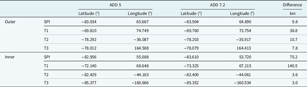
Our two algorithms agreed to within a few metres of each other. Results are summarised in Table 1, which shows the coordinates of the SPIs and the corresponding tangent points. Results are given in decimal degrees (north and east positive), with a precision of 0.001 degree (around 0.1 km in latitude) The table also shows the difference between the ADD v5 and ADD v7.2 positions, in kilometres. The distances from the outer SPIs to the outer coasts are 1588.6 km in ADD5 and 1590.4 km in ADD7.2; the corresponding distances for the inner coasts are 1242.8 and 1179.4 km respectively. Calculations using ADD7.4 gave essentially identical results to those using ADD7.2 (the largest difference noted for any of the positions reported in Table 1 was less than 1 m). Calculations repeated using ADD1-4 gave essentially identical results to those calculated using ADD5 for the outer coastline (all calculated distances were within 2 m of those reported in Table 1). For the inner coastline, the position of the calculated SPI varied by up to 3 km relative to the ADD5 value, although the positions of the tangent points T1 and T2 exhibited greater variability.
Table 1. Coordinates of the Southern Pole of Inaccessibilities (SPIs) and tangent points in decimal degrees (north and east positive), and differences between ADD5 and ADD7.2 positions in kilometres, for both outer and inner coasts.
Positions of the calculated SPIs and tangent points are shown in Figure 1, together with other locations of the SPI reported in the literature. The figure also shows the circles, centred on the SPI and passing through the corresponding tangent points. Figure 2 shows enlargements around the tangent points. The inner and outer coast tangent points labelled T1 are around the Amery Ice Shelf, while T2 are around the Ronne-Filchner Ice Shelf and T3 around the Ross Ice Shelf.
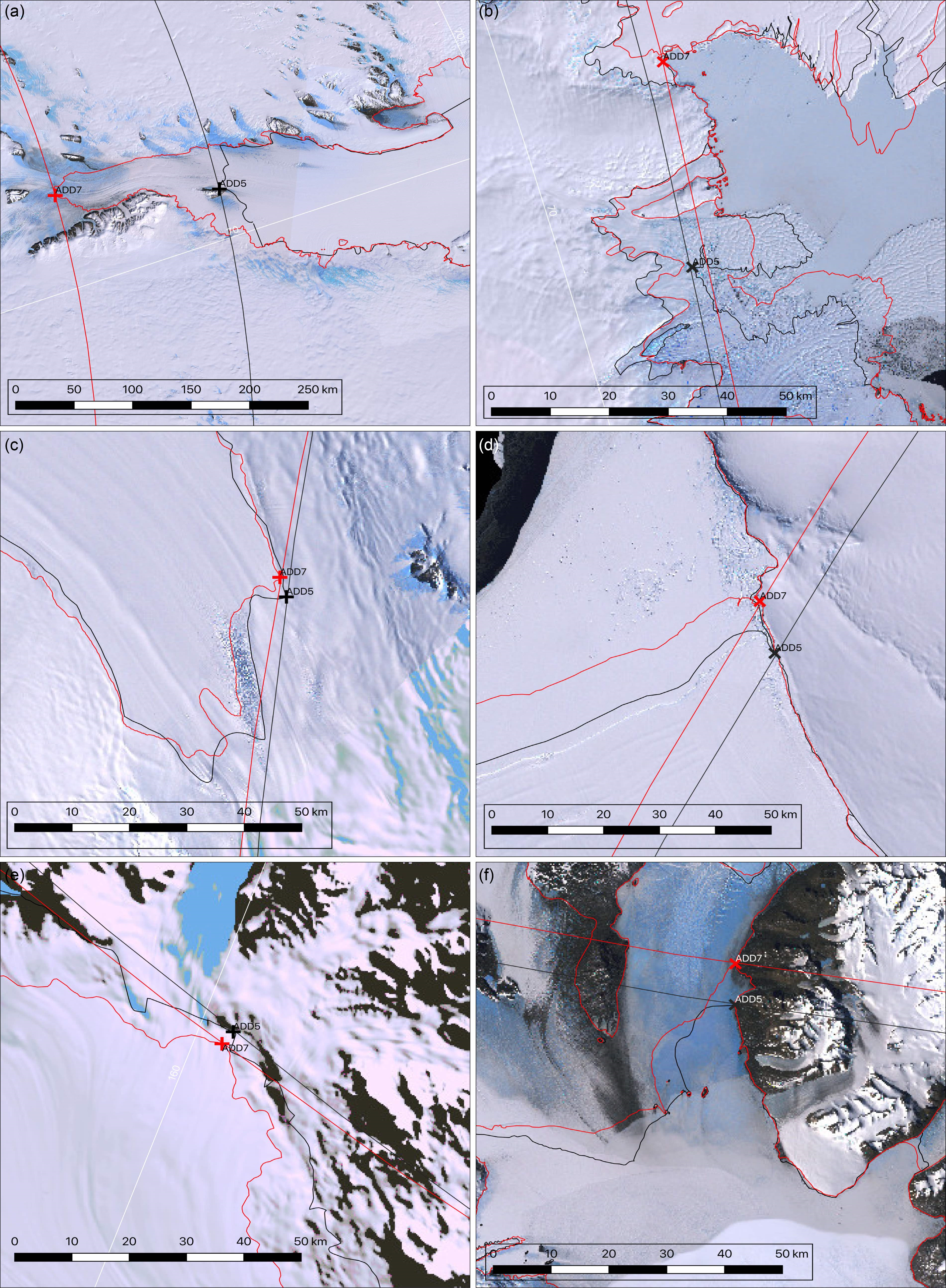
Fig. 2. Coastlines, tangent points and equidistant circles in the vicinity of T1 (Amery Ice Shelf; a and b), T2 (Ronne-Filchner Ice Shelf; c and d) and T3 (Ross Ice Shelf; e and f). Left (a, c and e): inner coast; right (b, d and f): outer coast. Black = ADD5, Red = ADD7.2. Background: Centre-filled LIMA (Landsat Image Mosaic of Antarctica: Bindschadler et al. Reference Bindschadler, Vornberger, Fleming, Fox, Mullins, Binnie and Gorodetzky2008).
Discussion
Examining first the tangent points on the outer coast, we can say that the shifts in position are plausible. The change in configuration of the Ronne-Filchner and Ross Ice Shelves between the two ADDs is relatively simple and coherent in form, and has resulted in shifts in position of the tangent points of the order of 10 km, consistent with the observed expansion of these ice shelves of around 1–2 km per year (e.g. Patel, Shah, Jayaprasad, & James, Reference Patel, Shah, Jayaprasad and James2020). The relevant geometry of the Amery Ice Shelf is more complex, and the shift is larger but again appears to be real. No major calvings occurred from the Amery Ice Shelf between 1964 and 2019 (Walker, Becker, & Fricker, Reference Walker, Becker and Fricker2021) and its behaviour during the time represented by this investigation was generally northwards expansion. The revision dates of the coastlines are not quite the same in all cases. The ADD5 coasts at T1, T2 and T3 are from 2000, 2005 and 1993, respectively, and the ADD7.2 coasts are from 2007, 2015 and 2020, respectively, so we can say that the mean rates of change in these positions are around 5 km per year for T1, and less than 1 km per year for T2 and T3. The corresponding rate of change in the position of the SPI is of the order of 1 km per year. We believe it is reasonable to assume that these positions are all accurate to within something of the order of 1 km, so that the rate of change is meaningfully different from zero. Although the latest data available for the T1 point are from 2007, the Amery Ice Shelf’s boundary was relatively unchanged until the calving of iceberg D28 in 2019 (Walker et al. Reference Walker, Becker and Fricker2021), which implies that the movement of the outer SPI would have been relatively constant during this period.
The tangent points on the inner coastline tell a different story. Two of them (T2 and T3) show very small shifts in position, while T1 shows a shift of well over 100 km. However, this is very likely to be an artefact of the improvement in the ability to map the grounding line of the Amery Ice Shelf (e.g. Fricker at al. Reference Fricker, Allison, Craven, Hyland, Young, Coleman and Popov2002). We can therefore not conclude that there is any evidence for a shift in the position of the inner SPI.
While we maintain that differences in position of both the SPIs and the corresponding tangent points between ADD5 and ADD7.2 (i.e. as reported in Table 1) are meaningful, methodological differences in obtaining them probably mean that variation in position of the inner SPI observed in earlier versions of the ADD is not meaningful. Previous statements about the position of the SPI can be interpreted in the light of these results. The positions attributed to BAS (2005: https://web.archive.org/web/20160414194423/http://www.explorersweb.com/polar/news.php?id=1298) for both the inner and outer SPIs are not essentially different (Fig. 1(b)) from those derived from ADD5 in this work. The Polar Heritage position for the inner SPI is also similar. The position of the inner SPI in other cases is unreliable.
Conclusions
The SPI (Antarctic Pole of Inaccessibility) is currently located at 83° 54’ S, 64° 53’ E, defined by the outer coast of Antarctica, and has been shifting its position at a rate of around 1 km per year since the early 21st century, as a result of changes in the Amery, Ronne-Filchner and Ross Ice Shelves. This point recently had a minimum distance of 1590 km from the coast, although it is probable that the 2019 calving of iceberg D28 from the Amery Ice Shelf will have shifted its position noticeably. The SPI defined from the inner coast is located at 83° 37’ S, 53° 43’ E and is a minimum distance of 1179.4 km from the inner coast. Although it appears to have shifted its position by around 75 km in the last decade, most if not all of this shift is likely to be due to improvements in our ability to map the position of the inner coast.
Competing interests
The authors declare that they have no competing interests.


 Open access