1. Introduction

The sea-ice cover in the polar oceans both affects and is affected by the overlying atmosphere. The sea ice restricts exchanges of heat, mass, and momentum between ocean and atmosphere, whereas the atmospheric temperatures and winds affect the freezing of the water and the melting and transport of the ice. In a recent paper Reference AckleyAckley (1981) reviews previous work on sea-ice/atmosphere relationships in the Southern Ocean. In some of the studies reviewed the change in Ice cover appears to result from atmospheric conditions and in other studies to cause them, for example, reduced ice cover intensifying cyclonic activity. The availability of several years of almost continuous global coverage by satellite now permits these interactions to be better defined. In an effort to examine year-to-year variations in sea ice and ice/atmosphere interactions, monthly sea-ice concentrations derived from satellite data have been compared for the three years 1973 to 1975 and these have been further compared with atmospheric temperature and pressure fields.

2. Data sets

3. Annual trends of temperature, pressure, and sea-ice extent

For an initial overall comparison of atmospheric fields and sea-ice extent, the mean latitude of the ice edge was calculated for each 3-day period of available data, and the mean temperatures and mean pressures over the latitude belt of the seasonal seaice cover, 60°S to 70°S, were also calculated for each 3-day period (Figs. 1-3). The ice-edge data reveal a strong, smooth yearly cycle, with minimum ice extent occurring in February and maximum ice extent occurring in September or October. The decay of the ice, which takes place over approximately 5 months, is decidedly more rapid than the growth, a point noted and discussed in several recent studies (Reference Rayner and HowarthRayner and Howarth 1979, Reference Lemke, Trinkl and HasselmannLemke and others 1980, Reference AckleyAckley 1981, Reference Cavalieri and ParkinsonCavalieri and Parkinson 1981). This contrasts with the situation found by Reference Walsh and JohnsonWalsh and Johnson (1979) in the Arctic and by Reference DeyDey (1980) specifically in Baffin Bay, where the growth is more rapid than the decay. For no 3-day period with available data do any pair of the 3 years examined differ by as much as 1 in the latitude of the mean ice edge (Fig.l).

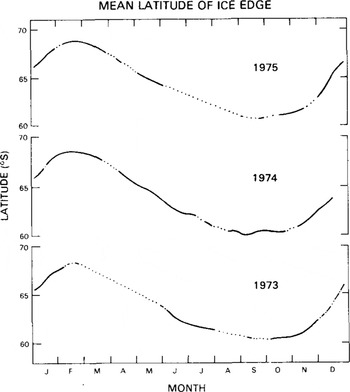
Fig.1. Annual cycle of the mean latitude of sea-ice extent in the Southern Ocean, 1973–75. The dotted portions of the curve signify time periods for which insufficient ESMR sea ice data are available.

The temperature data also show a clear yearly cycle (Fig.2), though this is far less smooth than the cycle for the ice edge (Fig.l). The temperature field appears to lead the ice field by 1 to 1.5 months, with maximum temperatures occurring several weeks before minimum ice extents and minimum temperatures occurring several weeks before maximum ice extents. (Relatedly, Reference Lemke, Trinkl and HasselmannLemke and others (1980) find the sea-ice maximum to lag the solar radiation minimum by 1.5 to 3 months, dependent upon longitude.) This reflects the stronger inertia of the ice. The mean temperatures exhibit considerably more interannual variability than do the mean ice-edge positions. In 1973 and 1974 temperatures peak in late December and early January and reach their minima in late July. In 1975 the temperatures reach a higher and sharper peak in mid-January and a broader minimum in August and September. Marked warmings occur in early May, late May, and late June 1975, and in late June 1974. Many of these warmings are of about two weeks' duration (Fig.2), which is typical of large-scale atmospheric wave fluctuations. Such warmings have been explained by Reference Van LoonVan Loon (1967), who demonstrates that during the months April to June an increase in wave activity, particularly in the Australian sector, results in the advection of warm air into high latitudes and often reverses the seasonal cooling.

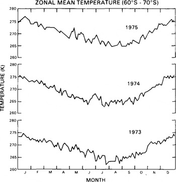
Fig.2. Annual cycle of zonal mean temperature for 60°S to 70°S, 197–5.

The zonal mean temperature maxima vary from 275 K to 276 K to 277 K and the minima vary from 262 K to 263 K to 265 K in 1973, 1974, and 1975, respectively, offering a rough suggestion of a 1 Ka⁻¹ warming over these years. In view of the wide-scale data interpolation necessitated by the sparsity of weather stations in the 60°S-70°S region, this 1 K interannual temperature change may be within the noise of the data. On the other hand, since it does represent an average over an entire latitude band, and since it is apparent in both the maximum and minimum temperatures, it may not be insignificant. There is a small coincident 197–5 increase in the latitude of minimum ice extent, from 68.3°S to 68.6°S to 68.9°S, consistent with the January-February temperature differences; but the gaps in the ice data prevent determining whether a corresponding trend exists in the latitude of maximum ice extent. A more definitive analysis of the apparent summertime association would require examination of the data on a regional basis, especially since the summer ice is dominated so strongly by certain regions (in particular, those in the western hemisphere). Certainly the zonal mean data do not show as strong an ice response to the temperature as that found by Reference BuddBudd (1975) for interannual variations in maximum ice extent versus annual mean temperatures at Laurie Island.

In contrast to temperature and sea-ice extent, zonal mean sea-level pressure (Fig.3) does not exhibit a strong yearly cycle. Instead, there is some indication of a semi-annual pressure variation consistent with that noted at 65°S by Reference Van LoonVan Loon (1967). This semi-annual variation reflects the semi-annual oscillation in the position of the circumpolar trough. In all three years, both the highest and lowest mean pressures occur during winter months, the highest occurring in July or August and the lowest in August or September. The mean pressures are almost all within the range 980 to 1 000 mbar, with the highest value (1 005 mbar in early August) and the lowest value (976 mbar in mid-September) both occurring in 1974. It is possible that the slightly earlier initiation of ice retreat in 1974 than in 1973 (Fig.l) is related to the lower mean pressures in September 1974, as intensified cyclonic activity would contribute to breaking up the ice cover.

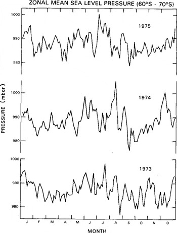
Fig.3. Annual cycle of zonal mean sea level pressure for 60°S to 70°S, 197–5.

4. Interannual sea-ice variations and atmospheric influences

The small amount of interannual variation in the mean latitudinal position of the Southern Ocean sea-ice edge over the years 197–5 (Section 3) contrasts sharply with the large amount of interannual variation apparent in the ice concentrations when these are mapped spatially. This large variation occurs on many time scales, including the monthly scales depicted here through maps of interannual differences in monthly-averaged ice concentrations. For each month with available ESMR data in both 1973 and 1974, the monthly-averaged ice concentrations for 1973 were subtracted, grid square by grid square, from those of 1974. In order to display detail both in the regions having more ice in 1973 and in the regions having more ice in 1974, maps generated from these data are presented in pairs, one map for each of the two sets of regions. The same procedure was followed for comparing ice conditions in 1974 and 1975. Some of the general points apparent from the maps, a few of which appear in Figure 4, are the following: (1) in each month and with each pair of years, there are millions of square kilometers with greater sea-ice amount in the first year and also millions of square kilometers with lesser ice amount, (2) for no month does one year have uniformly more or less ice than another year; i.e., the interannual differences are strongly spatially-dependent, (3) strong spatial coherence exists in the winter months, with lesser spatial coherence in the summer months of December and January, when the ice cover is decaying.

Examination of the sea-ice maps in conjunction with monthly averages of sea-level pressures and 1 000 mbar temperatures yields numerous examples of apparent atmospheric influences on interannual sea-ice differences. In many cases, the year-to-year differences in the positioning of low pressure systems and high pressure ridges correlate closely with the year-to-year differences in the ice. To illustrate various types of correspondences we have selected a few regions of interest in a summer month (January), in an ice-growth period (June-July), and at the time of maximum ice (September)

In January 1973, but in neither 1974 nor 1975, a prominent extension of ice exists to the north-east of the Antarctic Peninsula (Figs.4(a)-4(d)). This ice extension can be readily explained by the low pressure system which occurs in the Weddell Sea in the mean January sea-level pressure field for 1973 (Fig.5(a)) but not for 1974 or 1975. The winds, moving roughly clockwise around the low, advect cold air to the north-east of the peninsula, inhibiting rapid ice decay, and contribute a wind stress term encouraging transport of ice to lower latitudes. The greater ice extent in 1973 in turn contributes to the colder air temperatures by restricting the transfer of heat from the ocean and by providing a cold surface over which the advecting air is cooled. Indeed, the mean monthly temperatures north-east of the peninsula are 1 K to 2 K colder in 1973 than in either 1974 or 1975 (temperature maps not shown).

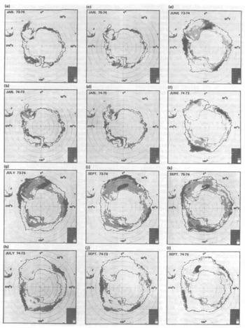
Fig.4. Monthly ice concentration differences, calculated by subtracting ESMR-derived mean monthly ice concentrations for corresponding months in different years, (a) January differences 197–4 for those regions with more ice in 1973 than in 1974; (b) January differences 1974-73 for those regions with more ice in 1974 than in 1973; (c) to (1) labeled similarly to (a) and (b). The 1974 ice edge is indicated in each map by a dashed line.

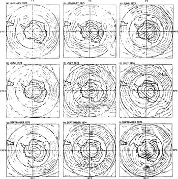
Fig.5. Monthly mean sea-level pressures.

Persistent features in the atmospheric fields are reflected in the zonal mean curves (Figs.2 and 3) as well as in the monthly maps (Fig.5). An example of such a feature in January 1975 is the poleward curving of the isobars in the South Pacific at about 170°E (Fig.5(b)). This pressure pattern presumably caused advection of warm air into the 60°S to 70°S latitude band, contributing to the significantly higher zonal mean temperature for the month (Fig.2) and thereby influencing the maximum latitude attained by the mean ice extent in that year. As discussed in section 3, this 1975 maximum latitude exceeds that attained in either of the other two years, signifying a lesser ice amount (Fig.l).

For June, the ice difference maps exhibit a strong longitudinal wave 3 pattern of contrasts between the years 1973 and 1974 (Figs.4(e) and 4(f)). At least some of the differences correspond well with the respective pressure fields (Figs.5(c) and 5(d)): the strong pressure gradient in the Bellingshausen Sea in 1974 suggests warm air advection and thereby explains the failure of the ice to advance as far northward as in June 1973, when no such pressure gradient existed; the 10°W to 40°w 1974 Weddell Sea pressure gradient suggesting south winds and cold air advection is consistent with the greater growth of ice there in 1974, and the greater growth off Enderby Land (30°E to 75°E) in 1974 can also be explained by the low to the east. No corresponding contrast in the positioning of low pressure systems can explain the prominent interannual ice differences in the outer reaches of the Ross Sea, but the stronger zonal flow associated with the more intense Ross Sea low in June 1973 probably contributes to the much lower ice concentration in that year.

Although, as noted by Reference AckleyAckley (1981), it is impossible with ice maps alone to differentiate definitively between thermodynamic and dynamic processes, it is conceivable that greater ice transport from the Ross to the Bellingshausen-Amundsen seas in June 1973 than in June 1974 created the interannual contrasts in the June ice extents and concentrations in these regions (Figs.4(e) and 4(f)). The possibility of west-to-east ice transport in June 1973 was noted earlier by Reference Zwally, Parkinson, Carsey, Gloersen, Campbell, Ramseier and KreinsZwally and others (1979) and disputed by Reference AckleyAckley (1981). However, Ackley's argument that the dominant winds in these latitudes should be the polar easterlies is not substantiated by a comparison of the latitudes of the ice edge (60°S to 70°S, Figs.4(e) and 4(f)) and the June pressure field (Fig.5(c)).

The amount of ice in a given month naturally depends heavily on the amount in the previous month as well as on atmospheric variables. To illustrate this, we center our discussion of the July ice-difference maps (Figs.4(g) and 4(h)) on their contrasts with the June maps (Figs.4(e) and 4(f)). Many of the changes from June to July can be explained by the positioning of three intense lows centered at 70°S, 0°E, 63°S, 120°E, and 65°S, 140°W in July 1973 (Fig.5(e)). To the west of each of the three lows, one would expect a stronger increase in ice concentrations in July of 1973 than in July of 1974, when the lows were significantly weaker. At least as reflected In the June-to-July transition (Figs.4(e) to 4(h)), this is true In each of the three cases: (1) in the northern Weddell Sea, the June ice concentrations were greater In 1974 but the July concentrations were greater 1n 1973, (2) In the northern Ross Sea the June concentrations were very much greater 1n 1974, but the July concentrations were only mildly greater In 1974, (3) at 90°E, the June concentrations were slightly greater 1n 1973 but the July concentrations were significantly greater 1n 1973. Similarly, to the east of each of the three major lows of Figure 5(e), one would.expect from the atmospheric circulation a lesser Increase In ice concentrations In July of 1973 than In July of 1974. As reflected In the June-to-July transition (Figs.4(e) to 4(h)), this 1s true for two of the three lows, those at 120°E and 140°W.

The dramatic shift off Wilkes Land (120°E to 160°E) from greater June Ice concentrations in 1973 to greater July concentrations In 1974 is consistent with the high pressure ridge located at 170°E in July 1973. This ridge, 1n combination with the two adjacent low pressure centers, suggests strong warm air advection Into the region In July 1973, leading to some decay of the ice cover. A discussion both of the influence of the blocking high over South America in July 1973 (Fig.5(e)) on decreasing the ice concentrations in the Bellingshausen Sea area and of the probable influence of the altered Ice conditions on creating, sustaining, or strengthening atmospheric lows can be found in Ackley and Keliher (1976).

The September pressure maps for 1973 and 1974 (F1gs.5(g) and 5(h)) are characterized by weak low pressure centers near the Antarctic coast and by predominantly zonal flow further toward the equator. The zonal winds are generally stronger in 1974 than in 1973 in the proximity of the 1ce edge, particularly in the 90°E to 180°E sector. These stronger westerlies in 1974, plus the meridional component of the 1973 winds at 135°E, provide an explanation for the sharp regional contrast observed in the ice, i.e., the fact that 1n the western portion of the 90°E to 180°E sector more 1ce exists in 1973 than In 1974, whereas In the eastern portion more 1ce exists in 1974 (Figures 4(i) and 4(j)). Similarly, the low pressure system centered in the Ross Sea (70°S, 180°E) 1n September 1975 could explain the lesser concentrations along the Ice edge in the Amundsen Sea (Fig.4(k)), although fluctuations In the position of the Antarctic Circumpolar Current cannot be ruled out as a contributing cause (Reference Zwally, Wilheit, Gloersen and MuellerZwally and others 1976). Another major Interannual contrast visible in the September Ice maps occurs in the region of the Weddell polynya (absent in 1973, centered at 0°E, 67°S in 1974, centered at 20°W, 67°S in 1975). Being unable to explain this polynya on the basis of the atmospheric fields, we refer the reader to recent studies examining possible oceanographic causes (Reference GordonGordon 1978, Reference CarseyCarsey 1980, Reference Martinson, Killworth and GordonMartinson and others 1981).

The fact that in September the ice concentrations were much lower in 1974 than in 1973 or 1975 (Figs.4(i) to 4(l)) is consistent with the greater variability in the pressure field in September 1974 (Fig.3), as the rapid passage of intense low pressure systems could be expected to maintain a lower ice concentration. This phenomenon of lower September ice concentrations in 1974 persists somewhat into October but not into November or December (images not shown).

5. Discussion

Selected features of the ice-atmosphere system over the three years 1973 to 1975 have been described using ESMR ice data and Australian southern hemisphere temperature and pressure data. Discussion has been basically restricted to large space and time scales because of the inherent difficulties in the atmospheric data, which, in contrast to the satellite derived ice data, are smoothed from very nonuniformly spaced stations with an unfortunately low density over sea-ice regions. The resulting uncertainty in the exact positioning of the temperature contours and the centering and intensity of low pressure systems makes some more detailed, quantitative analyses unwarranted, although such analyses are certainly desirable, and are in the planning stages, for the more data-dense FGGE year 1979.

Both the 60°S to 70°S zonal mean atmospheric temperature and the mean latitude of the ice edge exhibit strong yearly cycles over the 197–5 period, with the ice lagging the temperature field by about 1 to 1.5 months. Although the mean ice edge undergoes considerably less interannual variation than either the pressure or temperature, the variations that do exist are consistent with the temperature contrasts.

Regionally, the ice varies significantly among the years 197–5. Interannual differences in monthly ice concentration presented for 197–4 and 1974-75 show these variations generally to be coherent spatially on scales of several hundred kilometers and to exhibit patterns in which large regions with greater ice in one of two years are adjacent to large regions with greater ice in the other year. This fact alone shows that analysis of records predominantly from one or two regions can produce distorted impressions of possible climatic change if conclusions are extrapolated from these regions to the Southern Ocean as a whole. Furthermore, the difference maps demonstrate that the spatial patterns can change significantly from one month to the next.

Even with the data-sparse atmospheric analyses available, there are strong indications that the large-scale features of the interannual ice differences, in particular the tendency for alternating large regions of heavier and lighter ice near the ice edge in one year vs another, often result from the interannual changes in the positioning and intensity of cyclonic and anticyclonic systems. Other large-scale features presumably result from oceanographic systems, and from the interactions among the ice, the atmosphere, and the ocean.

Acknowledgements

The authors thank personnel from Computer Sciences Corporation for their assistance in generating the plots used in this study, Greg Walters of the National Center for Atmospheric Research for supplying the digitized southern hemisphere data from the Australian Bureau of Meteorology, and Tracy Pepin for her care in typing repeated versions of the manuscript. This research was supported by NASA's Climate Program in the Environmental Observations Division.