


1. Introduction and rationale
Recent progress in defining the standard cosmological model—known as  $\Lambda$
CDM—has been dominated by observations of the Cosmic Microwave Background (CMB, Hinshaw et al. Reference Hinshaw2013; Planck Collaboration et al. Reference Planck2016a, Reference Planck2018). Maps of the microwave sky made by the Planck satellite between 30 and 857 GHz have allowed almost cosmic variance limited measurements of the temperature anisotropy spectrum out to multipoles in excess of
$\Lambda$
CDM—has been dominated by observations of the Cosmic Microwave Background (CMB, Hinshaw et al. Reference Hinshaw2013; Planck Collaboration et al. Reference Planck2016a, Reference Planck2018). Maps of the microwave sky made by the Planck satellite between 30 and 857 GHz have allowed almost cosmic variance limited measurements of the temperature anisotropy spectrum out to multipoles in excess of  $\ell=1\,000$
as well as high fidelity measurements of the polarisation of the CMB. These measurements have constrained five of the standard six parameters
$\ell=1\,000$
as well as high fidelity measurements of the polarisation of the CMB. These measurements have constrained five of the standard six parameters  $\Lambda$
CDM to 1% precision and the final one (the optical depth to reionisation) to 10%. The parameter constraints from CMB observations are broadly compatible with other cosmological indicators such as measurements of the cosmic distance scale using standard candles such as Cepheids and Supernovae (Astier et al. Reference Astier2006) and number counts of clusters of galaxies (Planck Collaboration et al. Reference Collaboration2016c).
$\Lambda$
CDM to 1% precision and the final one (the optical depth to reionisation) to 10%. The parameter constraints from CMB observations are broadly compatible with other cosmological indicators such as measurements of the cosmic distance scale using standard candles such as Cepheids and Supernovae (Astier et al. Reference Astier2006) and number counts of clusters of galaxies (Planck Collaboration et al. Reference Collaboration2016c).
A wide range of physical phenomena can be probed beyond the  $\Lambda$
CDM model. These include the dark sector which is responsible for cosmic acceleration, massive neutrinos, and Primordial Non-Gausianity (PNG). Although these phenomena can be constrained with further observations of the CMB, probes of large-scale structure (LSS), mapping the Universe at relatively lower redshifts, are essential to break some of the degeneracies inherent in CMB observations.
$\Lambda$
CDM model. These include the dark sector which is responsible for cosmic acceleration, massive neutrinos, and Primordial Non-Gausianity (PNG). Although these phenomena can be constrained with further observations of the CMB, probes of large-scale structure (LSS), mapping the Universe at relatively lower redshifts, are essential to break some of the degeneracies inherent in CMB observations.
Measurements of the matter power spectrum through galaxy redshift surveys have been around for some time (Cole et al. Reference Cole2005), indeed before the detection of the CMB anisotropies, and have played a significant role in defining  $\Lambda$
CDM (Efstathiou, Sutherland, & Maddox Reference Efstathiou, Sutherland and Maddox1990). The next two decades will see rapid progress in the field of LSS surveys with the advent of the Euclid Satellite (Laureijs et al. Reference Laureijs2011a), the Large Synoptic Survey Telescope (LSST, LSST Science Collaboration et al. Reference Science Collaboration2009), the Dark Energy Spectroscopic Instrument (DESI, DESI Collaboration et al. Reference Collaboration2016), and the Wide-Field Infrared Survey Telescope (WFIRST, Akeson et al. Reference Akeson2019), which will create large-scale maps of the Universe. In particular, they will use measurements of the angular positions and redshifts of galaxies to infer the matter power spectrum, facilitating measurements of Baryonic Acoustic Oscillations (BAOs) and redshift space distortions (RSDs), and measurements of cosmic shear power spectrum by estimation of galaxy shapes. There are many challenges in achieving the fantastic levels of statistical precision which will be possible with these instruments, notably reducing the levels of observational systematic errors.
$\Lambda$
CDM (Efstathiou, Sutherland, & Maddox Reference Efstathiou, Sutherland and Maddox1990). The next two decades will see rapid progress in the field of LSS surveys with the advent of the Euclid Satellite (Laureijs et al. Reference Laureijs2011a), the Large Synoptic Survey Telescope (LSST, LSST Science Collaboration et al. Reference Science Collaboration2009), the Dark Energy Spectroscopic Instrument (DESI, DESI Collaboration et al. Reference Collaboration2016), and the Wide-Field Infrared Survey Telescope (WFIRST, Akeson et al. Reference Akeson2019), which will create large-scale maps of the Universe. In particular, they will use measurements of the angular positions and redshifts of galaxies to infer the matter power spectrum, facilitating measurements of Baryonic Acoustic Oscillations (BAOs) and redshift space distortions (RSDs), and measurements of cosmic shear power spectrum by estimation of galaxy shapes. There are many challenges in achieving the fantastic levels of statistical precision which will be possible with these instruments, notably reducing the levels of observational systematic errors.
The Square Kilometre ArrayFootnote a (SKA) is an international project to build a next-generation radio observatory which will ultimately have a collecting area of  $10^{6}\,{\hbox{m}}^2$
, i.e. the collecting area necessary to detect the neutral hydrogen (HI) emission at 21 cm from an
$10^{6}\,{\hbox{m}}^2$
, i.e. the collecting area necessary to detect the neutral hydrogen (HI) emission at 21 cm from an  $L_{*}$
galaxy at
$L_{*}$
galaxy at  $z\sim 1$
in a few hours (Wilkinson 1991). The SKA will comprise of two telescopes: a dish array (SKA-MID) based in the Northern Cape province of South Africa, and an array of dipole antennas (SKA-LOW) based near Geraldton in Western Australia, with the international headquarters on the Jodrell Bank Observatory Site in the United Kingdom. There will be two phases to the project dubbed SKA1 and SKA2 with a cost cap of
$z\sim 1$
in a few hours (Wilkinson 1991). The SKA will comprise of two telescopes: a dish array (SKA-MID) based in the Northern Cape province of South Africa, and an array of dipole antennas (SKA-LOW) based near Geraldton in Western Australia, with the international headquarters on the Jodrell Bank Observatory Site in the United Kingdom. There will be two phases to the project dubbed SKA1 and SKA2 with a cost cap of  $\sim$
675 MEuros being set for the SKA1. Only when SKA2 is built, will the SKA live up to its name.
$\sim$
675 MEuros being set for the SKA1. Only when SKA2 is built, will the SKA live up to its name.
The science case for the SKA has been presented in some detail in two volumes produced in 2015 (Braun et al. Reference Braun, Bourke, Green, Keane and Wagg2015), with 18 separate chapters presenting the cosmology science case for the SKA (see Maartens et al. Reference Maartens, Abdalla, Jarvis and Santos2015 for the overview chapter). The aim of this Red Book is to present the status of this science case, with updated forecasts based on the now agreed instrumental design of SKA1, to the cosmology community and beyond. We will not attempt to make detailed forecasts for SKA2 since its precise configuration is yet to be decided; suffice to say that it will have a significant impact on cosmology when it comes online. Furthermore, this is not intended to be a complete review of the subject area, rather it is a summary of the main science goals. We refer the reader to the individual papers for many of the details of the individual science cases.
The observations we will focus on here are:
Continuum emission largely due to synchrotron emission from electrons moving in the magnetic field of galaxies. Selecting galaxies in this way will allow the measurements of the positions and shapes of galaxies.
Line emission due to the spin-flip transition between the hyperfine states of neutral hydrogen (HI) at 21 cm. Using the redshifted HI line, it is possible to perform spectroscopic galaxy redshift surveys and also to use a new technique called Intensity Mapping (IM) whereby one measures the large-scale correlations in the HI brightness temperature without detecting individual galaxies.
Note that it should be possible to perform continuum and line surveys at the same time, also referred to as commensal observations, and that it may be possible to use the line emission of the galaxies to deduce redshifts, at least statistically, for the continuum galaxy samples.Footnote b
In this Red Book, we aim to update previous performance forecasts of the SKA Science Book for Phase 1 and to study the synergies between the SKA1 and future LSS experiments such as Euclid, LSST, and DESI focusing on cosmological parameters which are particularly well constrained by LSS measurements. In order to constrain the full set of cosmological parameters, many of which are already well constrained by the CMB, we also use Planck priors for our forecasts, which is a conservative choice and avoids making assumptions about the future progression of CMB measurements. These will improve and should provide more precise measurements of the standard set of parameters, but it is well understood that it is necessary to include LSS data to break the degeneracies inherent in the CMB power spectrum. Furthermore, we have already pointed out that the next generation of LSS surveys will be affected by significant observational systematic biases. The addition of radio observations by the SKA could be crucial to achieving the most reliable constraints from LSS, as cross-correlating the distribution and shapes of galaxies in two different wavebands will heavily suppress systematic effects. This is because one only expects weak correlations between the contaminants in the different wavebands. Furthermore, additional wavebands can lead to a host of other synergies, a topic we will return to in the discussion section.
2. Cosmological surveys with SKA1
In this section, we will present the specifications of SKA1 telescopes required for forecasting cosmological parameters, adopting the SKA1 Design Baseline in accordance with SKA-TEL-SKO-0000818Footnote c (Anticipated SKA1 Science Performance). In addition, we will define the fiducial cosmological model.
2.1. SKA1-MID
SKA1-MID will be a dish array consisting of a set of sub-arrays. The first is the South African SKA precursor MeerKAT which has 64 13.5 m diameter dishes which will be supplemented by 133 SKA1 dishes with 15 m diameter. These will be configured with a compact core and three logarithmically spaced spiral arms with a maximum baseline of  $150\,{{\text{km}}}$
which corresponds to an angular resolution of
$150\,{{\text{km}}}$
which corresponds to an angular resolution of  $\sim$
0.3 arcsec at a frequency of
$\sim$
0.3 arcsec at a frequency of  $1.4\,{\text{GHz}}$
. The details of the telescope configuration are presented in Table 1. It is planned that ultimately, these dishes will be equipped with receivers sensitive to 5 different frequency ranges or bands. The frequency ranges and, where appropriate, the redshift range for HI line observations are tabulated in Table 2.Footnote d In the present SKA baseline configuration, there are only sufficient funds to deploy Bands 1 and 2, which are most relevant to cosmology, and Band 5.
$1.4\,{\text{GHz}}$
. The details of the telescope configuration are presented in Table 1. It is planned that ultimately, these dishes will be equipped with receivers sensitive to 5 different frequency ranges or bands. The frequency ranges and, where appropriate, the redshift range for HI line observations are tabulated in Table 2.Footnote d In the present SKA baseline configuration, there are only sufficient funds to deploy Bands 1 and 2, which are most relevant to cosmology, and Band 5.
Table 1. Summary of the array properties of SKA1-MID which will comprise purpose-built SKA dishes and those from the South African precursor instrument, MeerKAT.

Table 2. Receiver bands on SKA1-MID. Included also is the range of redshift these receiver bands will probe using the 21-cm spectral line.

The overall system temperature for the SKA1-MID array can be calculated using
 \begin{equation}T_{{\text{sys}}}=T_{{\text{rx}}}+T_{{\text{spl}}}+T_{{\text{CMB}}}+T_{{\text{gal}}}\,,\end{equation}
where we have ignored contributions from the atmosphere.  $T_{{\text{spl}}}\approx 3\,{\text{K}}$
is the contribution from spill-over,
$T_{{\text{spl}}}\approx 3\,{\text{K}}$
is the contribution from spill-over,  $T_{{\text{CMB}}}\approx 2.73\,{\text{K}}$
is the temperature of the CMB,
$T_{{\text{CMB}}}\approx 2.73\,{\text{K}}$
is the temperature of the CMB,  $T_{{\text{gal}}}\approx 25\,{\text{K}}(408\,{\text{MHz}}/f)^{2.75}$
is the contribution of our own galaxy at frequency f, and
$T_{{\text{gal}}}\approx 25\,{\text{K}}(408\,{\text{MHz}}/f)^{2.75}$
is the contribution of our own galaxy at frequency f, and  $T_{{\text{rx}}}$
is the receiver noise temperature. In Band 1, we will assume
$T_{{\text{rx}}}$
is the receiver noise temperature. In Band 1, we will assume
 \begin{equation}T_{{\text{rx}}}=15\,{\text{K}}+30\,{\text{K}}\left(\frac{f}{{\text{GHz}}}-0.75\right)^2\,,\end{equation}
and in Band 2  $T_{{\text{rx}}}=7.5\,{\text{K}}$
.
$T_{{\text{rx}}}=7.5\,{\text{K}}$
.
2.2. SKA1-LOW
The SKA1-LOW interferometer array will consist of 512 stations, each containing 256 dipole antennas observing in one band at  $0.05\,{\text{GHz}}<\nu<0.35\,{\text{GHz}}$
. Most of the large-scale sensitivity comes from the tightly packed ‘core’ configuration of the array with
$0.05\,{\text{GHz}}<\nu<0.35\,{\text{GHz}}$
. Most of the large-scale sensitivity comes from the tightly packed ‘core’ configuration of the array with  $N_{d} = 224$
stations; however, the long baselines will be crucial for calibration and foreground removal. We assume that the core stations are uniformly distributed out to a 500-m radius, giving a maximum baseline
$N_{d} = 224$
stations; however, the long baselines will be crucial for calibration and foreground removal. We assume that the core stations are uniformly distributed out to a 500-m radius, giving a maximum baseline  $D_{{\text{max}}} = 1\, {{\text{km}}}$
. The station size is
$D_{{\text{max}}} = 1\, {{\text{km}}}$
. The station size is  $D =40\, {{\text{m}}}$
, the area per antenna is
$D =40\, {{\text{m}}}$
, the area per antenna is  $3.2\,{{\text{m}}}^2$
at 110 MHz, and the instantaneous field of view is
$3.2\,{{\text{m}}}^2$
at 110 MHz, and the instantaneous field of view is  ${(1.2 \, \lambda /D)^2}$
sr, with
${(1.2 \, \lambda /D)^2}$
sr, with  $\lambda = 21(1+z) \, {{\text{cm}}}$
. Although multi-beaming should be possible, we consider the conservative case of one beam only. The system temperature is given by
$\lambda = 21(1+z) \, {{\text{cm}}}$
. Although multi-beaming should be possible, we consider the conservative case of one beam only. The system temperature is given by  $T_{{\text{sys}}} = T_{{\text{rx}}}+T_{{\text{gal}}}$
, with the receiver temperature
$T_{{\text{sys}}} = T_{{\text{rx}}}+T_{{\text{gal}}}$
, with the receiver temperature  $T_{{\text{rx}}} = 0.1T_{{\text{gal}}}+40 \, {\text{K}}$
, and
$T_{{\text{rx}}} = 0.1T_{{\text{gal}}}+40 \, {\text{K}}$
, and  $T_{{\text{gal}}}$
defined as for SKA-MID.
$T_{{\text{gal}}}$
defined as for SKA-MID.
2.3. Proposed cosmology surveys
In this document, we will refer to the following surveys targeting cosmology with the SKA:
Medium-Deep Band 2 Survey: SKA1-MID in Band 2 covering 5 000
 ${{\text{deg}}}^2$
and an integration time of approximately
$t_{{\text{tot}}}= 10\,000$
h on sky. Main goals: a continuum weak lensing survey and an HI galaxy redshift survey out to
$z\sim 0.4$
(see Sections 3.2 and 4).
${{\text{deg}}}^2$
and an integration time of approximately
$t_{{\text{tot}}}= 10\,000$
h on sky. Main goals: a continuum weak lensing survey and an HI galaxy redshift survey out to
$z\sim 0.4$
(see Sections 3.2 and 4).Wide Band 1 Survey: SKA1-MID in Band 1 covering
$20\,000\,{{\text{deg}}}^2$
and an integration time of approximately
$t_{{\text{tot}}}= 10\,000$
h on sky. Main goals: a wide continuum galaxy survey and HI IM in the redshift range z = 0.35–3 (see Sections 3.3, 3.4 and 5).Deep SKA1-LOW Survey: This survey will naturally follow the Epoch of Reionisation (EoR) survey strategy. Currently, a three-tier survey consisting of a wide-shallow, a medium-deep, and a deep survey is planned. For our forecasts in this paper, we have assumed a deep-like survey with
$100 {\text{\, deg}}^2$
sky coverage and an integration time of approximately
$t_{{\text{tot}}}= 5\,000$
h on sky using data from sub-bands at frequencies 200–350 MHz, equivalent to
$3<z<6$
(see Section 5).


We emphasise that these are surveys which the Cosmology Science Working Group (SWG) is suggesting should be done as part of the SKA Key Science Program (KSP) which is currently envisaged to start  $\sim$
2028. A key feature of the KSP will be commensality with other science programmes; the ones which are most relevant are those convened under the auspices of the Continuum SWG, the Magnetism SWG, and the HI in galaxies SWG, all of which have the goal of understanding the physical properties of the objects we are proposing to use as cosmological indicators. In this paper, we have not presented analyses which attempt to optimise the output of the surveys and have relied on various previous studies in choosing, for example, the survey area and depth.
$\sim$
2028. A key feature of the KSP will be commensality with other science programmes; the ones which are most relevant are those convened under the auspices of the Continuum SWG, the Magnetism SWG, and the HI in galaxies SWG, all of which have the goal of understanding the physical properties of the objects we are proposing to use as cosmological indicators. In this paper, we have not presented analyses which attempt to optimise the output of the surveys and have relied on various previous studies in choosing, for example, the survey area and depth.
2.4. Survey processing requirements
The production of SKA data products will be performed by the Science Data Processor (SDP) element through High Performance Computer facilities at Perth and Cape Town for SKA1-LOW and SKA1-MID, respectively. The SKA1 Design Baseline for the telescope will deliver a compute power of 260 PFLOPs to deliver the science data products that will be transported to Regional Data Centres for further analysis. However, in order to meet the overall telescope cost cap, a Deployment Baseline has been defined which will deliver only 50 PFLOPs of compute power when telescope operations start, with a plan to increase to the full capability then being delivered over a 5-yr period. Although it is already planned that scientific programmes will be scheduled to spread the computational load across a period defined by the SDP ingest buffer, here we assess the computational load that will result from the surveys defined in Section 2.3. This assessment is based upon document SKA-TEL-SKO-0000941Footnote e (Anticipated SKA1 HPC Requirements).
Medium-Deep Band 2 Survey: This survey will require approximately 2 h of observing time on each individual field. Since the survey is assumed to be commensal with the project to create and an all sky rotation measure map to probe the galactic magnetic field, data products for all 4 polarisations will be required. The weak lensing experiment (Section 3.2) requires use of the longest baselines (150 km). The HI galaxy redshift survey requires that spectral line data products are generated in addition to the continuum ones needed for other purposes. Although combining these various requirements would seem to imply a maximally difficult data processing task, one of the key findings of SKA-TEL-SKO-0000941 is that the dominant computational cost is driven by the calibration step and that after this has been achieved, the delivery of multiple different science products to address their differing requirements at minimal incremental cost. Assuming that observations are only required in sub-band Mid sb4 (as defined in SKA-TEL-SKO-0000941), we therefore estimate that the computational cost of this experiment is approximately 75 PFLOPs (assuming 10% efficiency). While sb4 observations are sufficient for most continuum science goals, note that this would only cover  $z>0.2$
for HI galaxy surveys, and additional sb5 observations doubling the computational cost might be necessary.
$z>0.2$
for HI galaxy surveys, and additional sb5 observations doubling the computational cost might be necessary.
Wide Band 1 Survey: The primary data products required for the HI IM experiment (Section 5) are the antenna auto-correlations, potentially complemented with additional calibration derived from the shortest interferometer baselines. The compute power needed for processing autocorrelation data is negligible compared with that for visibility data. This survey will also be used to generate the Band 1 continuum source sample discussed in Section 3. The total observing time on each individual field is around 1 h, so the analysis in SKA-TEL-SKO-0000941 suggests that the computational cost of this survey is approximately 50 PFLOPs (assuming 10% efficiency) for each of the three sub-bands in Band 1 that are desired. However, as discussed in Section 5, in order to beat down systematic errors on the autocorrelation measurements, a fast scanning strategy may be adopted for this survey. Commensality with the continuum survey will then require an on-the-fly observing mode for the interferometer.Footnote f Although it seems technically feasible to implement such mode with SKA1-MID up to scanning speeds of 1 deg s−1, further assessments are still needed on the calibration requirements for the continuum survey and on the extra computational costs.
Deep SKA1-LOW Survey: This survey consists of more than 1 000 h integrations on a small number of individual fields with observations being commensal with the EoR Key Science Project (KSP). The computational load of calibrating such deep observations is not only severe, but is also a strong function of frequency across the SKA1-LOW band, with 200–350 MHz being substantially easier than 50–200 MHz. Although the signal of interest resides on the shortest baselines, it is likely that high angular resolution image data products will be required in order to remove the effects of contamination of discrete radio sources in the field, so we assume that baselines out to 65 km will need to be processed. We therefore estimate that the computational load for the 200–350 MHz survey is approximately 130 and 70 PFLOPs (assuming 10% efficiency) for sub-bands LOW sb5 and sb6. It should be noted that if these observations are performed commensally with the EoR, the requirement 24 for the Low sb 1,2,3,4 data are approximately 200, 300, 200, and 200 PFLOPs (assuming 10% efficiency), respectively.
In conclusion, if balanced against other projects with low computational demands such as the pulsar search and timing, then both the Medium-Deep Band 2 Survey should be feasible to conduct even with the reduced capability offered by the Deployment Baseline. The Wide IM survey by itself will not be constrained by computational demands, but commensality with the Wide continuum source survey requires further assessments depending on the scanning strategy. Observing a single sub-band of the Wide Band 1 Survey should be feasible with the initial HPC capability, but processing all three sub-bands simultaneously will be challenging until the HPC capability increases. The Deep SKA1-LOW Survey will be more problematic and may need to wait until the HPC capability increases. A caveat to this is that the EoR observing is planned to be conducted in only the best ionospheric conditions, or approximately 15% of the total available time, so potentially this work can start before the full Design Baseline capability is realised.
2.5. Synergies with other surveys
SKA cosmology will greatly benefit from synergies with optical surveys. Throughout this paper, we refer to the classification of surveys in the report of the Dark Energy Task Force (DETF, Albrecht et al. Reference Albrecht2009), which describes dark energy research developing in stages. Stage III comprises current and near-term projects, which improve the dark energy figure of merit by at least a factor of 3 over previous measurements; representatives of cosmic shear and galaxy clustering Stage III DETF experiments are, respectively, the Dark Energy Survey (DES) and SDSS Baryon Oscillation Spectroscopic Survey (BOSS). It is also customary to categorise Phase 1 of the SKA as Stage III. Stage IV experiments increase the dark energy figure of merit by at least a factor of 10 over previous measurements; Euclid, LSST and the full SKA stand as Stage IV observational campaigns. In the following, we outline various optical experiments suggested for synergies with the SKA1 throughout this document.
The Stage III DES explores the cosmic acceleration via four distinct cosmological probes: type Ia supernovae, galaxy clusters, BAO, and weak gravitational lensing. Over a 5 yr programme, it is covering  $5\,000\,{{\text{deg}}}^2$
in the Southern hemisphere, with a median redshift
$5\,000\,{{\text{deg}}}^2$
in the Southern hemisphere, with a median redshift  $z\approx 0.7$
(Dark Energy Survey Collaboration et al. Reference Collaboration2016).
$z\approx 0.7$
(Dark Energy Survey Collaboration et al. Reference Collaboration2016).
DESI is a Stage IV ground-based spectroscopic survey with 14 000 deg2 sky coverage (Aghamousa et al. Reference Aghamousa2016). It will use a number of tracers of the underlying dark matter field: luminous red galaxies up to  $z=1$
; emission line galaxies up to
$z=1$
; emission line galaxies up to  $z=1.7$
; and quasars and Ly-
$z=1.7$
; and quasars and Ly- $\alpha$
features up to
$\alpha$
features up to  $z=3.5$
. It plans to measure around 30 million galaxy and quasar redshifts and obtain extremely precise measurements of the BAO features and matter power spectrum in order to constrain dark energy and gravity, as well as inflation and massive neutrinos.
$z=3.5$
. It plans to measure around 30 million galaxy and quasar redshifts and obtain extremely precise measurements of the BAO features and matter power spectrum in order to constrain dark energy and gravity, as well as inflation and massive neutrinos.
The Euclid satellite is a European Space Agency’s medium class astronomy and astrophysics space mission. It comprises of two different instruments: a high-quality panoramic visible imager; and a NIR 3-filter (Y, J and H) photometer (NISP-P) together with a slitless spectrograph (NISP-S) (see Markovic et al. Reference Markovic2017 for details on the survey strategy). With these instruments, Euclid will probe the expansion history of the Universe and the evolution of cosmic structures, by measuring the modification of shapes of galaxies induced by gravitational lensing, and the three-dimensional distribution of structures from spectroscopic redshifts of galaxies and clusters of galaxies (Laureijs et al. Reference Laureijs2011b; Amendola et al. Reference Amendola2013, Reference Amendola2018).
The LSST is a forthcoming ground-based, wide field survey telescope. It will examine several probes of dark energy, including weak lensing tomography and BAOs. The LSST survey will cover  $18\,000\,{{\text{deg}}}^2$
, with a number density of galaxies
$18\,000\,{{\text{deg}}}^2$
, with a number density of galaxies  $40\,{{\text{arcmin}}}^{-2}$
, redshift range
$40\,{{\text{arcmin}}}^{-2}$
, redshift range  $0 < z < 2$
with median redshift
$0 < z < 2$
with median redshift  $z \approx 1$
(LSST Dark Energy Science Collaboration Reference Dark Energy2012).Footnote g
$z \approx 1$
(LSST Dark Energy Science Collaboration Reference Dark Energy2012).Footnote g
WFIRST was the highest rank large space project in the 2010 US Decadal Survey. The 2.4 m WFIRST is the same size telescope as the venerable Hubble Space Telescope but will operate hundreds of times faster due the 0.28 square degree ‘wide-field instrument’, which performs optical and NIR imaging and NIR grism spectroscopy using 16 Teledyne H4RG detectors. WFIRST will launch in late 2025 for a 5-yr primary mission that will have a dedicated wide-field surveys for cosmology, deep, high cadence surveys for SN detection and follow-up as well as exoplanet microlensing, and a General Observer programme that will allow the worldwide community to propose surveys for WFIRST (Akeson et al. Reference Akeson2019).
In addition, we note that on the timescale of the proposed observations, there will have been evolution also in the CMB observations which might be used to break degeneracies between cosmological parameters. These might include those which will come from the Simons Observatory (Ade et al. Reference Ade2019) and the CMB S4 projects (Abazajian et al. Reference Abazajian2016).
2.6. Fiducial cosmological model and extensions
The standard cosmological model that we have used is a  $\Lambda$
CDM model based on the the parameters preferred by the 2015 Planck analysis (TTTEEE + lowP). In particular, the physical baryon and cold dark matter (CDM) densities are
$\Lambda$
CDM model based on the the parameters preferred by the 2015 Planck analysis (TTTEEE + lowP). In particular, the physical baryon and cold dark matter (CDM) densities are  $\Omega_{b}h^2=0.02225$
and
$\Omega_{b}h^2=0.02225$
and  $\Omega_{c}h^2=0.1198$
, the value of the Hubble constant is
$\Omega_{c}h^2=0.1198$
, the value of the Hubble constant is  $H_0=100h\,{{\text{km}}}\,{{\text{s}}}^{-1}\,{\text{Mpc}}^{-1}=67.27\,{{\text{km}}}\,{{\text{s}}}^{-1}\,{\text{Mpc}}^{-1}$
, the amplitude and spectral index of density fluctuations are given by
$H_0=100h\,{{\text{km}}}\,{{\text{s}}}^{-1}\,{\text{Mpc}}^{-1}=67.27\,{{\text{km}}}\,{{\text{s}}}^{-1}\,{\text{Mpc}}^{-1}$
, the amplitude and spectral index of density fluctuations are given by 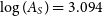 $\log(A_{S})=3.094$
and
$\log(A_{S})=3.094$
and  $n_{S}=0.9645$
, and the optical depth to reionisation is
$n_{S}=0.9645$
, and the optical depth to reionisation is  $\tau=0.079$
. We note that these parameter constraints were derived under the assumption that the sum of the neutrino masses is fixed to
$\tau=0.079$
. We note that these parameter constraints were derived under the assumption that the sum of the neutrino masses is fixed to 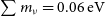 $\sum m_\nu=0.06\,{{\text{eV}}}$
and therefore we use this in the definition of our fiducial model.
$\sum m_\nu=0.06\,{{\text{eV}}}$
and therefore we use this in the definition of our fiducial model.
We also consider extensions to the standard model, focusing on those where addition of information from SKA1 can have an impact. Specifically, we will consider the following possibilities.
Curvature: parameterised by
$\Omega_{k}$
.Massive neutrinos: parameterised by the sum of the masses
$M_{\nu}=\sum m_{\nu}$
.Modifications to the dark sector equation of state: using the CPL parameterisation (Chevallier & Polarski Reference Chevallier and Polarski2001),
$P/\rho=w(a)=w_0+(1-a)w_a$
.Modified gravity: deviations from General Relativity (GR) can be encoded by an effective description of the relation between the metric potentials of the form
(3)
\begin{align} -2k^2\Psi&=8\pi G_Na^2 \mu(a,k) \rho \Delta,\end{align}
(4)where the GR limit is
\begin{align}\hspace*{-11pt}\frac{\Phi}{\Psi} &= \gamma(a,k),\end{align}
$\mu=\gamma=1$
and
$\Delta$
is the comoving density perturbation. We consider scale independent deviations from GR which emerge at late times (we neglect the effect at
$z>5$
), hence we assume they are proportional to the dark energy density parameter:
(5)
\begin{align}\mu(a,k) &= 1+\mu_0\frac{\Omega_\Lambda(a)}{\Omega_{\Lambda,0}},\end{align}
(6)
\begin{align}\gamma(a,k) &= 1+\gamma_0\frac{\Omega_\Lambda(a)}{\Omega_{\Lambda,0}}.\end{align}
$\mu_0$
and
$\gamma_0$
are the free parameters in our analysis.Non-Gaussianity: this is parameterised using the local
$f_{{\text{NL}}}$
defined in terms of the amplitude of the quadratic contributions to the metric potential
$\Phi$
as a local function of a single Gaussian field
$\phi$
,
(7)
\begin{equation}\Phi(x) = \phi(x) + f_{{\text{NL}}}\left(\phi^2(x)-\langle\phi^2\rangle\right) + \ldots\,.\end{equation}


At various stages during the analysis, we have imposed a Planck prior on our forecast cosmological parameter constraints. Unless stated otherwise, this is based on the Planck 2015 CMB + BAO + lensing results presented in Planck Collaboration et al. (Reference Planck2016a). This was implemented by taking published MCMC chainsFootnote h and calculating the covariance matrix for the following extended set of cosmological parameters:  $n_s$
,
$n_s$
,  $\sigma_8$
,
$\sigma_8$
,  $\Omega_b h^2$
,
$\Omega_b h^2$
,  $\Omega_m h^2$
, h,
$\Omega_m h^2$
, h,  $w_0$
, and
$w_0$
, and  $w_a$
. The covariance matrix was then inverted to obtain an effective Fisher matrix for the prior, which is marginalised over all other parameters (including nuisance parameters) that were included in the Planck analysis. Applying the prior is then simply a matter of adding it to the forecast Fisher matrix for the survey of interest. While this method is approximate (e.g. it discards non-Gaussian information from the Planck posterior), it is sufficiently accurate for forecasting.
$w_a$
. The covariance matrix was then inverted to obtain an effective Fisher matrix for the prior, which is marginalised over all other parameters (including nuisance parameters) that were included in the Planck analysis. Applying the prior is then simply a matter of adding it to the forecast Fisher matrix for the survey of interest. While this method is approximate (e.g. it discards non-Gaussian information from the Planck posterior), it is sufficiently accurate for forecasting.
3. Continuum galaxy surveys
3.1. Modelling the continuum sky
In this section, we outline how to model the continuum sky and the science cases for the Wide Band 1 Survey and Medium-Deep Band 2 Survey. The continuum flux density limit of the Medium-Deep Band 2 Survey is estimated to be 8.2  $\mu$
Jy assuming a 10
$\mu$
Jy assuming a 10 $\sigma$
r.m.s. detection threshold, whereas the Wide Band 1 Survey will cover four times the area, to approximately slightly less than half the depth, and the flux density limit is predicted to be more than double the Medium-Deep Band 2 Survey, at
$\sigma$
r.m.s. detection threshold, whereas the Wide Band 1 Survey will cover four times the area, to approximately slightly less than half the depth, and the flux density limit is predicted to be more than double the Medium-Deep Band 2 Survey, at  $22.8\,\mu$
Jy assuming a 10
$22.8\,\mu$
Jy assuming a 10 $\sigma$
r.m.s. detection threshold. Note that this is not exactly a factor of two different to that for the Medium-Deep Band 2 Survey since the overall sensitivity of the array varies with frequency.
$\sigma$
r.m.s. detection threshold. Note that this is not exactly a factor of two different to that for the Medium-Deep Band 2 Survey since the overall sensitivity of the array varies with frequency.
In Figure 1, we plot the expected number distribution as a function of redshift of all radio galaxies as well as split by galaxy type, for the two different surveys in the top and bottom panel, respectively. These distributions are generated using the SKA Simulated Skies ( $S^3$
) simulations,Footnote i based on Wilman et al. (Reference Wilman2008).
$S^3$
) simulations,Footnote i based on Wilman et al. (Reference Wilman2008).

Figure 1. The total and number of each galaxy species as function of redshift N(z) for a  $5\,000\,{{\text{deg}}}^2$
survey (above) and a
$5\,000\,{{\text{deg}}}^2$
survey (above) and a  $20\,000\,{{\text{deg}}}^2$
survey (below) on SKA1-MID, assuming a flux limit of 8.2
$20\,000\,{{\text{deg}}}^2$
survey (below) on SKA1-MID, assuming a flux limit of 8.2  $\mu$
Jy (for the Medium-Deep Band 2 Survey) and 22.8
$\mu$
Jy (for the Medium-Deep Band 2 Survey) and 22.8  $\mu$
Jy (for the Wide Band 1 Survey), both assuming 10
$\mu$
Jy (for the Wide Band 1 Survey), both assuming 10 $\sigma$
detection. The galaxy types are SFG, SB, Fanaroff-Riley type-I and type-II radio galaxies (FR1 & FR2), and radio-quiet quasars (RQQ).
$\sigma$
detection. The galaxy types are SFG, SB, Fanaroff-Riley type-I and type-II radio galaxies (FR1 & FR2), and radio-quiet quasars (RQQ).

Figure 2. Bias as a function of redshift for the different source types, as following the simulated  $S^3$
catalogues of Wilman et al. (Reference Wilman2008) including the cut-off above some redshift as described in the text.
$S^3$
catalogues of Wilman et al. (Reference Wilman2008) including the cut-off above some redshift as described in the text.
We also need to choose a model for the galaxy bias. Each of the species of source (i.e. starburst (SB), star-forming galaxy (SFG), FRI-type radio galaxy, etc.) from the  $S^3$
simulation has a different bias model, as described in Wilman et al. (Reference Wilman2008). The bias in these models increases continuously with redshift, which is unphysical at high redshift; to avoid this, we follow the approach of Raccanelli et al. (Reference Raccanelli2011) holding the bias constant above a cut-off redshift (see Figure 2). Having a handle on the redshift evolution of bias and structure will represent a strong improvement for radio continuum galaxy surveys, thanks to the high-redshift tail of continuum sources and will translate into tighter constraints on dark energy parameters compared to the unbinned case, as shown in Camera et al. (Reference Camera, Santos, Bacon, Jarvis, McAlpine, Norris, Raccanelli and Rottgering2012). The true nature of the bias for high-redshift, low-luminosity radio galaxies, remains currently unknown; the choice of a bias model therefore remains a source of uncertainty, but one that the SKA will be able to resolve.
$S^3$
simulation has a different bias model, as described in Wilman et al. (Reference Wilman2008). The bias in these models increases continuously with redshift, which is unphysical at high redshift; to avoid this, we follow the approach of Raccanelli et al. (Reference Raccanelli2011) holding the bias constant above a cut-off redshift (see Figure 2). Having a handle on the redshift evolution of bias and structure will represent a strong improvement for radio continuum galaxy surveys, thanks to the high-redshift tail of continuum sources and will translate into tighter constraints on dark energy parameters compared to the unbinned case, as shown in Camera et al. (Reference Camera, Santos, Bacon, Jarvis, McAlpine, Norris, Raccanelli and Rottgering2012). The true nature of the bias for high-redshift, low-luminosity radio galaxies, remains currently unknown; the choice of a bias model therefore remains a source of uncertainty, but one that the SKA will be able to resolve.
As well as predicting the number and bias of the galaxies for the two strategies, we also use the fluxes from the  $S^3$
simulation to predict values for the slope of the source-flux to number density power law, which couples the observed number density to the magnification (magnification bias), given by
$S^3$
simulation to predict values for the slope of the source-flux to number density power law, which couples the observed number density to the magnification (magnification bias), given by
 \begin{equation}\alpha_{{\text{mag}}}(S) = -\frac{d(\!\log n)}{d(\!\log S)}\,,\end{equation}
where S is the flux density and n is the unmagnified number density (Bartelmann & Schneider Reference Bartelmann and Schneider2001). Magnification bias arises because faint objects are more likely to be seen if they are magnified by gravitational lenses due to overdensities along the line of sight. This changes the clustering properties of the sample and thus contains cosmological information.
Table 3. For each redshift bins used in our analysis, we present the redshift range, expected number of galaxies, galaxy bias, and magnification bias ( $\alpha_{{\text{mag}}}$
), for the two continuum surveys. The bias refers to the number-weighted average of the bias of all galaxies in the bin. These surveys are expected to have a total angular number density
$\alpha_{{\text{mag}}}$
), for the two continuum surveys. The bias refers to the number-weighted average of the bias of all galaxies in the bin. These surveys are expected to have a total angular number density 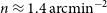 $n\approx 1.4\,{{\text{arcmin}}}^{-2}$
for the Wide Band 1 Survey and
$n\approx 1.4\,{{\text{arcmin}}}^{-2}$
for the Wide Band 1 Survey and  $\approx 3.2\,{{\text{arcmin}}}^{-2}$
for the Medium-Deep Band 2 Survey.
$\approx 3.2\,{{\text{arcmin}}}^{-2}$
for the Medium-Deep Band 2 Survey.

Finally, we will be able to divide our sample into redshift bins, based on photometric or statistical information (Kovetz, Raccanelli, & Rahman Reference Kovetz, Raccanelli and Rahman2017b; Harrison, Lochner, & Brown Reference Harrison, Lochner and Brown2017). While these bins will not be as accurate as spectroscopic redshifts, they will still allow us to recover some of the 3D information from the distribution of galaxies. The Medium-Deep Band 2 Survey will have cross-identifications from other wave-bands (optical from the DES, for example) over its smaller area, allowing for accurate photometric redshift bins, whereas the Wide Band 1 Survey will have limited all sky optical/IR information. We assume nine photo-z bins for Medium-Deep Band 2 Survey and five for Wide Band 1 Survey. The assumed redshift bin distribution, as well as the number of galaxies, bias, and slope of the source count power-law, is given in Table 3.
3.2. Weak lensing
A statistical measurement of the shapes of millions of galaxies as a function of sky position and redshift enables us to measure the gravitational lensing effect of all matter—dark and baryonic—along the line of sight between us and those galaxies. Weak lensing shear measurements are insensitive to factors such as galaxy bias. A number of studies have made marginal detections of the radio weak lensing signal (Chang, Refregier, & Helfand Reference Chang, Refregier and Helfand2004) and radio-optical cross correlation signals (Demetroullas & Brown Reference Demetroullas and Brown2016, Reference Demetroullas and Brown2018), but convincing detections have not yet been possible due to a lack of high number densities of resolved, high redshift sources (see Patel et al. Reference Patel, Bacon, Beswick, Muxlow and Hoyle2010; Tunbridge, Harrison, & Brown Reference Tunbridge, Harrison and Brown2016; Hillier et al. Reference Hillier, Brown, Harrison and Whittaker2018).
Here, we demonstrate the capabilities of SKA1 as a weak lensing experiment, both alone and in cross-correlation with optical lensing experiments. We consider only a total intensity continuum lensing survey, but note that useful information could also be gained on the important intrinsic alignment astrophysical systematic by using polarisation (Brown & Battye Reference Brown and Battye2010, Reference Brown and Battye2011; Thomas et al. Reference Thomas, Whittaker, Camera and Brown2017) and resolved rotational velocity (e.g. Morales Reference Morales2006) measurements.
3.2.1. Cosmic shear simulations for SKA
We create forecasts for the SKA1 Medium-Deep Band 2 Survey. This survey is very similar to the optimal observing configuration found from catalogue-level simulations in Bonaldi et al. (Reference Bonaldi, Harrison, Camera and Brown2016). We assume the survey will use the lower  $1/3$
of Band 2 and the weak lensing data will be weighted to give an image plane point spread function (PSF) width of
$1/3$
of Band 2 and the weak lensing data will be weighted to give an image plane point spread function (PSF) width of  $0.55\,{\text{arcsec}}$
, with the source population cut to include all sources which have flux
$0.55\,{\text{arcsec}}$
, with the source population cut to include all sources which have flux  $>10\sigma$
and a size
$>10\sigma$
and a size  $>$
1.5
$>$
1.5  $\times$
the PSF size. These source populations are also rescaled, as in Bonaldi et al. (Reference Bonaldi, Harrison, Camera and Brown2016), to more closely match more recent data and the T-RECS simulation (Bonaldi et al. Reference Bonaldi, Bonato, Galluzzi, Harrison, Massardi, Kay, De Zotti and Brown2018). For comparison to a similar Stage III optical weak lensing experiment, and for use in shear cross-correlations, we take the DES with expectations for the full 5-yr survey. The assumed parameters of the two surveys are fully specified in Table 4. For the Medium-Deep Band 2 Survey, we assume a sensitivity corresponding to baseline weighting resulting in an image plane PSF with a best-fitting Gaussian FWHM of
$\times$
the PSF size. These source populations are also rescaled, as in Bonaldi et al. (Reference Bonaldi, Harrison, Camera and Brown2016), to more closely match more recent data and the T-RECS simulation (Bonaldi et al. Reference Bonaldi, Bonato, Galluzzi, Harrison, Massardi, Kay, De Zotti and Brown2018). For comparison to a similar Stage III optical weak lensing experiment, and for use in shear cross-correlations, we take the DES with expectations for the full 5-yr survey. The assumed parameters of the two surveys are fully specified in Table 4. For the Medium-Deep Band 2 Survey, we assume a sensitivity corresponding to baseline weighting resulting in an image plane PSF with a best-fitting Gaussian FWHM of  $0.55\,{\text{arcsec}}$
.
$0.55\,{\text{arcsec}}$
.
Table 4. Parameters used in the creation of simulated weak lensing data sets for SKA1 Medium-Deep Band 2 Survey and DES 5-yr survey considered in this section.

We assume redshift distributions for weak lensing galaxies follow a distribution for the number density of the form
 \begin{equation}\frac{{\text{d}} n}{{\text{d}} z} \propto z^{2} \exp\left( -(z/z_0)^{\gamma} \right),\end{equation}
where  $z_0 = z_{m} / \sqrt{2}$
and
$z_0 = z_{m} / \sqrt{2}$
and  $z_{m}$
is the median redshift of sources using best fitting parameters for the SKA1-MID Medium-Deep Band 2 Survey population and DES survey given in Table 4. Sources are split into ten tomographic redshift bins, with equal numbers of sources in each bin and each source is attributed an error as follows. A fraction of sources
$z_{m}$
is the median redshift of sources using best fitting parameters for the SKA1-MID Medium-Deep Band 2 Survey population and DES survey given in Table 4. Sources are split into ten tomographic redshift bins, with equal numbers of sources in each bin and each source is attributed an error as follows. A fraction of sources  $f_{{\text{spec-}}z}$
out to a redshift of
$f_{{\text{spec-}}z}$
out to a redshift of  $z_{{\text{spec-max}}}$
are assumed to have spectroscopic errors, in line with the predictions of Yahya et al. (Reference Yahya, Bull, Santos, Silva, Maartens, Okouma and Bassett2015); Harrison et al. (Reference Harrison, Lochner and Brown2017). The remainder of sources are given photometric redshift errors with a Gaussian distribution (constrained with the physical prior
$z_{{\text{spec-max}}}$
are assumed to have spectroscopic errors, in line with the predictions of Yahya et al. (Reference Yahya, Bull, Santos, Silva, Maartens, Okouma and Bassett2015); Harrison et al. (Reference Harrison, Lochner and Brown2017). The remainder of sources are given photometric redshift errors with a Gaussian distribution (constrained with the physical prior  $z>0$
) of width
$z>0$
) of width  ${(1+z)\sigma_{{\text{photo-}}z}}$
out to a redshift of
${(1+z)\sigma_{{\text{photo-}}z}}$
out to a redshift of  $z_{{\text{photo-max}}}$
. Beyond
$z_{{\text{photo-max}}}$
. Beyond  $z_{{\text{photo-max}}}$
, we assume very poor redshift information, with
$z_{{\text{photo-max}}}$
, we assume very poor redshift information, with  ${(1+z)\sigma_{{\text{no-}}z}}$
.
${(1+z)\sigma_{{\text{no-}}z}}$
.
Of crucial importance to weak lensing cosmology is precise, accurate measurement of source shapes in order to infer the shear transformation resulting from gravitational lensing. For our forecasts, we assume systematic errors due to shear measurement will be sub-dominant to statistical ones. For the Medium-Deep Band 2 Survey, the formulae of Amara & Réfrégier (Reference Amara and Réfrégier2008) allow us to calculate requirements on the multiplicative shear bias of 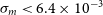 $\sigma_{m} < 6.4\times10^{-3}$
and additive shear bias of
$\sigma_{m} < 6.4\times10^{-3}$
and additive shear bias of  $\sigma_{c} < 8.0\times10^{-4}$
. These requirements are of the same order of magnitude as those achieved in current optical weak lensing surveys such as DES and the Kilo-Degree Survey,Footnote j but tighter (by an order of magnitude in the case of multiplicative bias) than current methods for radio interferometer to date (Rivi & Miller Reference Rivi and Miller2018; Rivi et al. Reference Rivi, Lochner, Balan, Harrison and Abdalla2018). We assume that in the period to 2028, when observations are currently expected to begin, sufficient progress will be made in radio shear measurement methods such that biases are comparable to those achievable in optical surveys today. Previous work has shown that this is highly unlikely to be possible with images created with the CLEAN algorithm (Högbom Reference Högbom1974) meaning access to lower level data products such as gridded visibilities (or equivalently dirty images) will be essential (see also Patel et al. Reference Patel2015; Harrison & Brown Reference Harrison and Brown2015). For the intrinsic ellipticity distribution of galaxies, we use a shape dispersion of
$\sigma_{c} < 8.0\times10^{-4}$
. These requirements are of the same order of magnitude as those achieved in current optical weak lensing surveys such as DES and the Kilo-Degree Survey,Footnote j but tighter (by an order of magnitude in the case of multiplicative bias) than current methods for radio interferometer to date (Rivi & Miller Reference Rivi and Miller2018; Rivi et al. Reference Rivi, Lochner, Balan, Harrison and Abdalla2018). We assume that in the period to 2028, when observations are currently expected to begin, sufficient progress will be made in radio shear measurement methods such that biases are comparable to those achievable in optical surveys today. Previous work has shown that this is highly unlikely to be possible with images created with the CLEAN algorithm (Högbom Reference Högbom1974) meaning access to lower level data products such as gridded visibilities (or equivalently dirty images) will be essential (see also Patel et al. Reference Patel2015; Harrison & Brown Reference Harrison and Brown2015). For the intrinsic ellipticity distribution of galaxies, we use a shape dispersion of  $\sigma_{g_i} = 0.3$
.
$\sigma_{g_i} = 0.3$
.

Figure 3. Forecast constraints for weak lensing with the SKA1 Medium-Deep Band 2 Survey as specified in the text, compared to the Stage III optical weak lensing DES and including cross-correlation constraints.
There are significant advantages to forming cosmic shear power spectra by cross-correlating shear maps made using two different experiments. In such power spectra, wavelength-dependent additive and multiplicative systematics can be removed (Camera et al. Reference Camera, Harrison, Bonaldi and Brown2017) and almost all of the statistical constraining power on cosmological parameters is retained (Harrison et al. Reference Harrison, Camera, Zuntz and Brown2016). Care must be taken in identifying the noise power spectra in the case of cross-power spectra; it will be affected by the overlap in shape information between cross-experiment bins. We note that constraints are relatively insensitive to the number of galaxies which are present in both bins, being degraded by only 4% when the fraction of overlap is varied between zero and one (see Harrison et al. Reference Harrison, Camera, Zuntz and Brown2016, Figure 1).
Table 5. One-dimensional marginalised constraints, from weak lensing alone and in combination with Planck CMB (Planck CMB2015 + BAO + lensing as described in Section 2.6), on the parameters considered, where all pairs (indicated by brackets) are also marginalised over the base ΛCDM parameter set.


Figure 4. The effect of including a prior from the Planck satellite (Planck 2015 CMB + BAO + lensing as described in Section 2.6) on the forecast Dark Energy constraints for the specified cross-correlation weak lensing experiment (note that constraints in the other two parameter spaces are not significantly affected).
3.2.2. Results from autocorrelation
We show forecast constraints in three cosmological parameter spaces in Figure 3: matter ( $\Omega_\textit{m}\hbox{-}\sigma_8$
), Dark Energy equation of state in the CPL parameterisation (
$\Omega_\textit{m}\hbox{-}\sigma_8$
), Dark Energy equation of state in the CPL parameterisation ( $w_0\hbox{-}w_a$
), and modified gravity modifications to the Poisson equation and Gravitational slip (
$w_0\hbox{-}w_a$
), and modified gravity modifications to the Poisson equation and Gravitational slip ( $\mu_0\hbox{-}\gamma_0$
). Our results show that the SKA1 Medium-Deep Band 2 Survey will be capable of comparable constraints to other DETF Stage III surveys such as DES and also, powerfully, that cross-correlation constraints (which are free of wavelength-dependent systematics) retain almost all of the statistical power of the individual experiments. In Figure 4, we also present forecast constraints in the Dark Energy parameter space including priors from the Planck CMB experiment, specifically a Gaussian approximation to the Planck 2015 CMB + BAO + lensing likelihood as described in Section 2.6 with constraints on the other parameters considered not significantly affected by application of the Planck prior. We note that future CMB experiments may improve their constraining power, the lowering the impact of the SKA measurements on this particular parameter space, however as outlined below, a major motivation for weak lensing in the radio is the independence of the systematics compared to measurements in the optical.
$\mu_0\hbox{-}\gamma_0$
). Our results show that the SKA1 Medium-Deep Band 2 Survey will be capable of comparable constraints to other DETF Stage III surveys such as DES and also, powerfully, that cross-correlation constraints (which are free of wavelength-dependent systematics) retain almost all of the statistical power of the individual experiments. In Figure 4, we also present forecast constraints in the Dark Energy parameter space including priors from the Planck CMB experiment, specifically a Gaussian approximation to the Planck 2015 CMB + BAO + lensing likelihood as described in Section 2.6 with constraints on the other parameters considered not significantly affected by application of the Planck prior. We note that future CMB experiments may improve their constraining power, the lowering the impact of the SKA measurements on this particular parameter space, however as outlined below, a major motivation for weak lensing in the radio is the independence of the systematics compared to measurements in the optical.
We also display tabulated summaries of the one-dimensional marginalised uncertainties on these parameters in Table 5.
3.2.3. Results for mixed-stage surveys
The current SKA timeline expects large surveys such as the Medium-Deep Band 2 Survey specified here to begin in 2027, by which time Stage III optical surveys such as DES will have been completed and analysed (DES data have been taken up to year 6 and the year 3 data release is currently being prepared. One may expect the 5-yr release to be in 2021). Stage IV optical surveys (LSST and the Euclid satellite) are currently scheduled to begin taking data in the middle years of the next decade, with the full data sets becoming available around 2030, possibly concurrent with those from SKA phase 1. We therefore also consider forecasts for mixed-stage cosmic shear surveys, with the radio data coming from SKA phase 1 Medium-Deep Band 2 Survey as described above, and optical data from the Stage IV LSST survey. Figure 5 shows the relevant contours for the  $\Omega_\textit m\hbox{-}\sigma_8$
parameters, with the expected significant gain when going from a Stage III to Stage IV survey. The contours from the SKA1-Medium-Deep Band 2 Survey
$\Omega_\textit m\hbox{-}\sigma_8$
parameters, with the expected significant gain when going from a Stage III to Stage IV survey. The contours from the SKA1-Medium-Deep Band 2 Survey  $\times$
LSST combination show degradation of constraints with respect to the LSST case, but will be significantly less susceptible to systematics, as discussed above and below in this section. For LSST, we assume a galaxy number density of
$\times$
LSST combination show degradation of constraints with respect to the LSST case, but will be significantly less susceptible to systematics, as discussed above and below in this section. For LSST, we assume a galaxy number density of  $n = 37\,$
arcmin–2 and a sky area of
$n = 37\,$
arcmin–2 and a sky area of  $18\,000\,$
deg2 and photometric redshifts only out to
$18\,000\,$
deg2 and photometric redshifts only out to  $z=3$
. For the cross-correlation, we consider only the
$z=3$
. For the cross-correlation, we consider only the  $5\,000\,$
deg2 SKA Medium-Deep Band 2 Survey area.
$5\,000\,$
deg2 SKA Medium-Deep Band 2 Survey area.

Figure 5. Forecast constraints for weak lensing with the SKA1 Medium-Deep Band 2 Survey as specified in the text, compared to the Stage IV optical weak lensing LSST survey and including cross-correlation. constraints.
3.2.4. Results from radio-optical cosmic shear cross-correlations
A key consideration in weak lensing surveys are the systematics induced by the instrument on galaxy shape measurements, which must be controlled to high levels in order to ensure unbiased constraints on cosmological parameters. In contrast with the optical weak lensing surveys conducted to date, radio weak lensing surveys will measure galaxy shapes from uv-data, allowing for direct Fourier plane measurement, as well as measurement in images reconstructed by deconvolving the interferometer PSF. The systematics from these shape measurements will be very different, and uncorrelated with, those from measuring shapes from CCD images. In Rivi & Miller (Reference Rivi and Miller2018), the authors adapted the optical method lensfit to shape measurement on Fourier-domain interferometer data which is capable of satisfying the requirements for the SKA1 Medium-Deep Band 2 Survey on sources with  ${\text{SNR}}>18$
. Residual systematics are typically modelled as linear in the shear and shear power spectrum, with an additive and multiplicative component. In Figure 3 (and Harrison et al. Reference Harrison, Camera, Zuntz and Brown2016), the unfilled black contours show the constraints from cross-correlating radio and optical weak lensing experiments, demonstrating that nearly all of the statistical constraining power remains.
${\text{SNR}}>18$
. Residual systematics are typically modelled as linear in the shear and shear power spectrum, with an additive and multiplicative component. In Figure 3 (and Harrison et al. Reference Harrison, Camera, Zuntz and Brown2016), the unfilled black contours show the constraints from cross-correlating radio and optical weak lensing experiments, demonstrating that nearly all of the statistical constraining power remains.
We explictly show this removal of systematics through cross-correlations in Figure 6 (and Camera et al. Reference Camera, Harrison, Bonaldi and Brown2017). Both panels show forecasts (made using Fisher matrices validated on the MCMC chains described above) for constraints on the  $\lbrace w_0, w_{a}\rbrace$
dark energy parameters. The upper panel shows the effect of systematics which are additive in the power spectrum, for a given choice of additive systematics power spectrum of fixed slope and varying amplitudes (see Camera et al. Reference Camera, Harrison, Bonaldi and Brown2017, for a full description of both this and the multiplicative power spectrum systematics models). As can be seen, such systematics significantly bias the recovered values of
$\lbrace w_0, w_{a}\rbrace$
dark energy parameters. The upper panel shows the effect of systematics which are additive in the power spectrum, for a given choice of additive systematics power spectrum of fixed slope and varying amplitudes (see Camera et al. Reference Camera, Harrison, Bonaldi and Brown2017, for a full description of both this and the multiplicative power spectrum systematics models). As can be seen, such systematics significantly bias the recovered values of  $\lbrace w_0, w_{a}\rbrace$
away from the input cosmology shown by the dashed cross. By construction, additive systematics are removed for the Radio
$\lbrace w_0, w_{a}\rbrace$
away from the input cosmology shown by the dashed cross. By construction, additive systematics are removed for the Radio  $\times$
Optical combination and the correct input cosmology is recovered. The lower panel shows the effect of systematics which are multiplicative in the power spectrum (i.e. are calibration systematics). Here, whilst the combined Radio
$\times$
Optical combination and the correct input cosmology is recovered. The lower panel shows the effect of systematics which are multiplicative in the power spectrum (i.e. are calibration systematics). Here, whilst the combined Radio  $\times$
Optical contour remains biased away from the input cosmology, the three separate contours available allow a self-calibration procedure to be applied; each contour has different systematics, but all are measuring the same cosmology, meaning a correction can be found which makes all three consistent with each other, and the input cosmology. Mitigation of such multiplicative systematics is expected to be extremely important even at the level of Stage III surveys and represents a powerful argument for performing weak lensing in the radio band.
$\times$
Optical contour remains biased away from the input cosmology, the three separate contours available allow a self-calibration procedure to be applied; each contour has different systematics, but all are measuring the same cosmology, meaning a correction can be found which makes all three consistent with each other, and the input cosmology. Mitigation of such multiplicative systematics is expected to be extremely important even at the level of Stage III surveys and represents a powerful argument for performing weak lensing in the radio band.

Figure 6. Weak lensing marginal joint 1 $\sigma$
error contours in the dark energy equation-of-state parameter plane with additive (top) and multiplicative (bottom) systematics on the shear power spectrum measurement. The black cross indicates the ΛCDM fiducial values for dark energy parameters. Blue, red, and green ellipses are for radio and optical/near-IR surveys and their cross-correlation, respectively. (Details in the text.)
$\sigma$
error contours in the dark energy equation-of-state parameter plane with additive (top) and multiplicative (bottom) systematics on the shear power spectrum measurement. The black cross indicates the ΛCDM fiducial values for dark energy parameters. Blue, red, and green ellipses are for radio and optical/near-IR surveys and their cross-correlation, respectively. (Details in the text.)
3.3. Angular correlation function and integrated Sachs–Wolfe effect
The angular distribution of galaxies and the cross-correlation of the galaxy positions with other tracers can yield important cosmological tests. The two-point distribution of radio galaxy positions in angle space can be represented by the angular correlation power spectrum  $C_{\ell}^{i,j}$
, where
$C_{\ell}^{i,j}$
, where  $\ell$
is the multipole number and i, j label redshift bins with the galaxies distributed across these bins defined by window functions,
$\ell$
is the multipole number and i, j label redshift bins with the galaxies distributed across these bins defined by window functions,  $W_i(z)$
. This statistic encodes the density distribution projected on to the sphere of the sky, and so smooths over structure along the line of sight. This can dampen the effect of RSDs on the angular power spectrum for broad redshift distributions, but these can become important as the distributions narrow (Padmanabhan et al. Reference Padmanabhan2007).
$W_i(z)$
. This statistic encodes the density distribution projected on to the sphere of the sky, and so smooths over structure along the line of sight. This can dampen the effect of RSDs on the angular power spectrum for broad redshift distributions, but these can become important as the distributions narrow (Padmanabhan et al. Reference Padmanabhan2007).
When two non-overlapping redshift bins are considered, the cross-correlation of density perturbations between these two bins measured through  $C_{\ell}^{i,j}$
will be negligible in the absence of lensing. However, the observed galaxy distribution is also affected by gravitational lensing through magnification, which can induce a correlation between the two bins, creating an observed correlation between the positions of some high redshift galaxies and the distribution of matter at low redshift.
$C_{\ell}^{i,j}$
will be negligible in the absence of lensing. However, the observed galaxy distribution is also affected by gravitational lensing through magnification, which can induce a correlation between the two bins, creating an observed correlation between the positions of some high redshift galaxies and the distribution of matter at low redshift.
The distribution of matter in the Universe can also be measured by the effect on the CMB temperature anisotropies, through the Integrated Sachs–Wolfe effect (ISW), where the redshifting and blueshifting of CMB photons by the intervening gravitational potentials generate an apparent change in temperature (Sachs & Wolfe Reference Sachs and Wolfe1967). Since the distribution of matter (which generates the gravitational potentials) can be mapped through the distribution of tracer particles, such as galaxies, the effect is detected by cross-correlating the positions of galaxies and temperature anisotropies on the sky. For a more detailed description of the use of the ISW with SKA continuum surveys, see Raccanelli et al. (Reference Raccanelli2015).
Here, we demonstrate the capabilities of SKA for using the angular correlation function and relevant cross-correlations as a cosmological probe.
3.3.1. Forecasting
In order to estimate the effectiveness of the surveys and make predictions for the constraints on the cosmological parameters, we simulate the auto- and cross-correlation galaxy clustering angular power spectra, including the effects of cosmic magnification and the ISW. As only the observed galaxy distributions (which are affected by gravitational lensing) can be measured, it is impossible to measure the galaxy angular power spectrum decoupled from magnification. Hence, the galaxy clustering angular power spectrum contains both the density and magnification perturbations.
We use the simulated source count and galaxy bias model from Section 3.1 to simulate the angular correlation and cross-correlation functions  $C_\ell$
, and the relevant measurement covariance matrices, for the Wide Band 1 Survey and Medium-Deep Band 2 Survey. In the case of galaxy clustering and ISW, we limit the analysis to the multipoles
$C_\ell$
, and the relevant measurement covariance matrices, for the Wide Band 1 Survey and Medium-Deep Band 2 Survey. In the case of galaxy clustering and ISW, we limit the analysis to the multipoles  $\ell_{{\text{min}}}\leq \ell\leq 200$
, where
$\ell_{{\text{min}}}\leq \ell\leq 200$
, where  $\ell_{{\text{min}}} = \pi/(2f_{{\text{sky}}})$
and
$\ell_{{\text{min}}} = \pi/(2f_{{\text{sky}}})$
and  $f_{{\text{sky}}}$
is the fraction of sky surveyed.
$f_{{\text{sky}}}$
is the fraction of sky surveyed.
When making our forecasts, we also compare to and combine with current constraints from Planck CMB 2015, BAO, and RSD observations, as described in Section 2.6 (with additional relevant information for the extension parameters under consideration). We also assume that the overall bias for a particular redshift bin to be unknown, and so marginalised over. As such there are five (or nine, depending on the number of photometric bins for the given survey) extra parameters being considered in the Fisher matrix, which will degrade the performance of these cosmological probes.
Table 6. Predicted constraints from continuum galaxy clustering measurements using the two different survey strategies (Wide Band 1 Survey and Medium-Deep Band 2 Survey). These are 68% confidence levels on each of the parameters of the four different cosmological models we tested. The three main columns show results of galaxy clustering (GC) by itself (left), GC combined with ISW constraints (centre), and when Planck priors from Planck CMB 2015 + BAO are added to GC + ISW (right). Note that these cases assume that the overall bias in each of the photometric redshift bins is unknown and needs to be marginalised over.

3.3.2. Results
The 68% confidence level constraints on the different parameters described in Section 2.6 for the Wide Band 1 Survey and the Medium-Deep Band 2 Survey are given Table 6.
We show the predicted 68% and 95% confidence level constraints as a 2D contour, for the dark energy parameters  $w_0$
and
$w_0$
and  $w_a$
in Figure 7, and the modified gravity parameters
$w_a$
in Figure 7, and the modified gravity parameters  $\mu_0$
and
$\mu_0$
and  $\gamma_0$
in Figure 8. These constraints are shown for the Wide Band 1 Survey and the Medium-Deep Band 2 Survey in red, combining measurements from all photometric redshift bins, and including constraints from the ISW. In the dark energy case, we also show current constraints from Planck in blue, but for the modified gravity case, the Planck MCMC chains for these models are not public.
$\gamma_0$
in Figure 8. These constraints are shown for the Wide Band 1 Survey and the Medium-Deep Band 2 Survey in red, combining measurements from all photometric redshift bins, and including constraints from the ISW. In the dark energy case, we also show current constraints from Planck in blue, but for the modified gravity case, the Planck MCMC chains for these models are not public.
The predicted constraints on the dark energy parameters do not improve significantly on those presently available. This is also somewhat the case for the modified gravity parameters and the curvature, in the case of the Medium-Deep Band 2 Survey, though the Wide Band 1 Survey does improve on current knowledge. However, such constraints will improve with a better knowledge of the bias (decreasing the number of extra parameters to be marginalised over) and with a larger number of photometric redshift bins.
Constraints on  $f_{{\text{NL}}}$
from the Medium-Deep Band 2 Survey will not be significantly better than those currently made by the Planck surveyor,
$f_{{\text{NL}}}$
from the Medium-Deep Band 2 Survey will not be significantly better than those currently made by the Planck surveyor,  $f_{{\text{NL}}} = 2.5 \pm 5.7$
(Planck Collaboration et al. Reference Collaboration2016Reference Planckb). In contrast, the Wide Band 1 Survey is capable of improving the constraint, with further potential gain from an increased number of redshift bins (Raccanelli et al. Reference Raccanelli2017). Finally, more competitive constraints on all parameters, but especially for
$f_{{\text{NL}}} = 2.5 \pm 5.7$
(Planck Collaboration et al. Reference Collaboration2016Reference Planckb). In contrast, the Wide Band 1 Survey is capable of improving the constraint, with further potential gain from an increased number of redshift bins (Raccanelli et al. Reference Raccanelli2017). Finally, more competitive constraints on all parameters, but especially for  $f_{{\text{NL}}}$
, may be achievable through the use of different radio galaxy populations as tracers of different mass halos, as described in Ferramacho et al. (Reference Ferramacho, Santos, Jarvis and Camera2014).
$f_{{\text{NL}}}$
, may be achievable through the use of different radio galaxy populations as tracers of different mass halos, as described in Ferramacho et al. (Reference Ferramacho, Santos, Jarvis and Camera2014).

Figure 7. 68% and 95% confidence level forecast constraints on the deviation of the dark energy parameters  $w_0,w_a$
from their fiducial values for the Wide Band 1 Survey (top) and Medium-Deep Band 2 Survey (bottom), using galaxy clustering data, including the effects of cosmic magnification. We show constraints from Planck CMB 2015 and BAO and RSD observations, as described in Section 2.6 in blue, SKA1 forecasts in red and the constraints for the combination of both experiments in green. We show here that for the dark energy parameters, the continuum data adds little to the existing constraints, owing to the uncertainty in the bias in each redshift bin. As such the blue Planck + BAO ellipse is only slightly bigger than the SKA + Planck + BAO for the continuum data. For the modified gravity parameters on the right, the Planck + BAO only chains were not available, and so the blue ellipse was left out of the figure.
$w_0,w_a$
from their fiducial values for the Wide Band 1 Survey (top) and Medium-Deep Band 2 Survey (bottom), using galaxy clustering data, including the effects of cosmic magnification. We show constraints from Planck CMB 2015 and BAO and RSD observations, as described in Section 2.6 in blue, SKA1 forecasts in red and the constraints for the combination of both experiments in green. We show here that for the dark energy parameters, the continuum data adds little to the existing constraints, owing to the uncertainty in the bias in each redshift bin. As such the blue Planck + BAO ellipse is only slightly bigger than the SKA + Planck + BAO for the continuum data. For the modified gravity parameters on the right, the Planck + BAO only chains were not available, and so the blue ellipse was left out of the figure.

Figure 8. 68% and 95% confidence level forecast constraints on the deviation of the modified gravity parameters  $\mu_0,\gamma_0$
from their fiducial values for the Wide Band 1 Survey (top) and Medium-Deep Band 2 Survey (bottom), using galaxy clustering data, including the effects of cosmic magnification. We show SKA forecasts constraints in red and the constraints for the combination of SKA1 with Planck CMB 2016 and BAO in green.
$\mu_0,\gamma_0$
from their fiducial values for the Wide Band 1 Survey (top) and Medium-Deep Band 2 Survey (bottom), using galaxy clustering data, including the effects of cosmic magnification. We show SKA forecasts constraints in red and the constraints for the combination of SKA1 with Planck CMB 2016 and BAO in green.
3.4. Cosmic dipole
The standard model of cosmology predicts that that the radio sky should be isotropic on large scales. Deviations from isotropy are expected to arise from proper motion of the Solar system with respect to the isotropic CMB (the cosmic dipole), the formation of LSSs and light propagation effects like gravitational lensing.
The CMB dipole is normally associated with the proper motion of the Sun with respect to the cosmic heat bath at  $T_0 = 2.725$
K. However, the CMB dipole could also contain other contributions, e.g. a primordial temperature dipole or an ISW effect, and measurements using only CMB data are limited by cosmic variance.
$T_0 = 2.725$
K. However, the CMB dipole could also contain other contributions, e.g. a primordial temperature dipole or an ISW effect, and measurements using only CMB data are limited by cosmic variance.
The extragalactic radio sky offers an excellent opportunity to perform an independent test of the origin of the cosmic dipole. It is expected that the radio dipole is dominated by the kinematic dipole, as radio continuum surveys have median redshifts well above one (unlike visible or infrared surveys). Current estimates of the radio dipole show good agreement with the CMB dipole direction, but find a dipole amplitude that is a factor of 2–5 larger than expected (Blake & Wall Reference Blake and Wall2002; Singal Reference Singal2011; Rubart & Schwarz Reference Rubart and Schwarz2013; Colin et al. Reference Colin, Mohayaee, Rameez and Sarkar2017; Bengaly, Maartens, & Santos Reference Bengaly, Maartens and Santos2018a). The current discrepancy between the measured radio dipole (from NVSS, SUMSS, WENSS, TGSS) and the CMB dipole is not understood. This anomaly might have a variety of reasons, among them some systematic effects in existing radio surveys, an unexpected distribution of the nearby LSS or a significant primordial CMB dipole that adds to the kinematic CMB dipole in such a way that it reduces it. In order to resolve this puzzle, a careful study of all systematics will be necessary, e.g. via using multi-frequency information and studying the direction and amplitude of the radio dipole as a function of flux density threshold. See also Bengaly et al. (Reference Bengaly, Siewert, Schwarz and Maartens2018b) for a study on dipole measurements with the SKA1 and SKA2.
3.4.1. Forecasting
In this section, we estimate the ability of SKA1 continuum surveys to measure the cosmic radio dipole using realistic mock catalogues, which include the effects of LSS and the kinematic dipole. Details of that study will be published elsewhere. Briefly, the mock catalogues assumed an angular power spectrum of the radio galaxies generated by CAMB sources (Challinor & Lewis Reference Challinor and Lewis2011), assuming the Planck best-fit flat  $\Lambda$
CDM model (Planck Collaboration et al. Reference Collaboration2016Reference Plancka). The redshift distribution N(z) is shown in Figure 1, and the bias b(z) follows Alonso et al. (Reference Alonso, Bull, Ferreira, Maartens and Santos2015b). The available sky area is
$\Lambda$
CDM model (Planck Collaboration et al. Reference Collaboration2016Reference Plancka). The redshift distribution N(z) is shown in Figure 1, and the bias b(z) follows Alonso et al. (Reference Alonso, Bull, Ferreira, Maartens and Santos2015b). The available sky area is  $f_{{\text{sky}}} \approx 0.52$
due to the removal of the galactic plane on low latitudes (
$f_{{\text{sky}}} \approx 0.52$
due to the removal of the galactic plane on low latitudes ( $|b| \leq 10^{\circ}$
). Using the lognormal code flask (Xavier, Abdalla, & Joachimi Reference Xavier, Abdalla and Joachimi2016), we produced ensembles of 100 catalogues each, where the radio source positions follow the expected clustering distribution.
$|b| \leq 10^{\circ}$
). Using the lognormal code flask (Xavier, Abdalla, & Joachimi Reference Xavier, Abdalla and Joachimi2016), we produced ensembles of 100 catalogues each, where the radio source positions follow the expected clustering distribution.
The effect of the kinetic dipole is implemented by boosting the maps of galaxy number densities according to the theoretical expectation (Ellis & Baldwin Reference Ellis and Baldwin1984),
 \begin{align}\left[\frac{{\text{d}} N}{{\text{d}}\Omega} (S, \mathbf{n})\right]_{{\text{obs}}} = \left[\frac{{\text{d}} N}{{\text{d}}\Omega} (S, \mathbf{n})\right]_{{\text{rest}}} \left( 1 + [2 + \beta (1+\alpha)] \frac{\mathbf{n}\cdot\mathbf{v}} {c}\right),\end{align}
where S denotes the flux density threshold of the survey,  $\mathbf{n}$
is the direction on the sky and
$\mathbf{n}$
is the direction on the sky and  $\mathbf{v}$
is the Sun’s proper motion. This expression assumes that radio sources follow a power-law spectral energy distribution,
$\mathbf{v}$
is the Sun’s proper motion. This expression assumes that radio sources follow a power-law spectral energy distribution,  $S \propto \nu^{-\beta}$
with
$S \propto \nu^{-\beta}$
with  $\beta = 0.75$
. The source counts are assumed to scale with S as
$\beta = 0.75$
. The source counts are assumed to scale with S as  $dn/dS\propto S^{-\alpha}$
, and we assume
$dn/dS\propto S^{-\alpha}$
, and we assume  $\alpha = 1$
(which is very similar to the values of
$\alpha = 1$
(which is very similar to the values of  $\alpha$
for the individual redshift bins from simulations given in Table 3).
$\alpha$
for the individual redshift bins from simulations given in Table 3).
Here, we show results from estimations of the radio dipole direction and amplitude,  $A = [2+ \beta(1+\alpha)]|\mathbf{v}|/c$
, of the generated mock catalogues by means of a quadratic estimator in pixel space on a HEALPixFootnote k grid with Nside = 64. Using pixel space has the advantage that incomplete sky coverage does not bias the results.
$A = [2+ \beta(1+\alpha)]|\mathbf{v}|/c$
, of the generated mock catalogues by means of a quadratic estimator in pixel space on a HEALPixFootnote k grid with Nside = 64. Using pixel space has the advantage that incomplete sky coverage does not bias the results.
3.4.2. Results
Figure 9 shows an example of a simulated sky for a flux density threshold of 22.8  $\mu$
Jy at a central frequency of 700 MHz (Band 1), demonstrating the effect of the dipole on the source counts, as the southern sky appears to be slightly more dominated by blue than the northern hemisphere. The results from a set of 100 such simulations is shown in Figure 10. Given the assumptions, we would expect our mocks to produce a kinematic radio dipole amplitude of
$\mu$
Jy at a central frequency of 700 MHz (Band 1), demonstrating the effect of the dipole on the source counts, as the southern sky appears to be slightly more dominated by blue than the northern hemisphere. The results from a set of 100 such simulations is shown in Figure 10. Given the assumptions, we would expect our mocks to produce a kinematic radio dipole amplitude of  $A = 0.0046$
, pointing to the CMB dipole direction. The LSS contributes a dipole with a mean amplitude of
$A = 0.0046$
, pointing to the CMB dipole direction. The LSS contributes a dipole with a mean amplitude of  $A = 0.0031 \pm 0.0016$
. This prediction depends on the assumed luminosity functions, spectral energy distributions, bias, redshift, and luminosity evolution of radio sources, see e.g. Tiwari & Nusser (Reference Tiwari and Nusser2016).
$A = 0.0031 \pm 0.0016$
. This prediction depends on the assumed luminosity functions, spectral energy distributions, bias, redshift, and luminosity evolution of radio sources, see e.g. Tiwari & Nusser (Reference Tiwari and Nusser2016).

Figure 9. Simulated source count per pixel for the SKA1-MID Wide Band 1 Survey at a central frequency of 700 MHz and a flux threshold of 22.8  $\mu$
Jy in galactic coordinates and Mollweide projection at HEALPix resolution
$\mu$
Jy in galactic coordinates and Mollweide projection at HEALPix resolution  $N_{{\text{side}}}=64$
including the kinematic dipole and cosmic structure up to multipole moment
$N_{{\text{side}}}=64$
including the kinematic dipole and cosmic structure up to multipole moment  $\ell_{{\text{max}}}=128$
. This shows the effect of the dipole on the source counts, as the southern sky appears here slightly bluer than the northern hemisphere.
$\ell_{{\text{max}}}=128$
. This shows the effect of the dipole on the source counts, as the southern sky appears here slightly bluer than the northern hemisphere.
Figure 10 shows the expected total radio dipole, which comprises contributions from LSS and the proper motion of the solar system. The expected kinematic contribution dominates the structure contribution and the measured amplitude is  $A = 0.0056 \pm 0.0017$
in direction
$A = 0.0056 \pm 0.0017$
in direction  $(l,b) = (263.5\pm 28.0, 38.8\pm 19.7)$
deg. The distribution of dipole directions from the mocks is centred on the CMB dipole direction, but with some scatter due to the LSS.
$(l,b) = (263.5\pm 28.0, 38.8\pm 19.7)$
deg. The distribution of dipole directions from the mocks is centred on the CMB dipole direction, but with some scatter due to the LSS.
The structure dipole is in fact dominated by contributions from local structure. Removing the low-redshift structure dipole ( $z < 0.5$
), which might be possible using optical or infra-red catalogues, or by means of the HI redshift measured by the SKA, we measure the dipole direction
$z < 0.5$
), which might be possible using optical or infra-red catalogues, or by means of the HI redshift measured by the SKA, we measure the dipole direction  $(l,b) = (265.3 \pm 4.9, 46.4 \pm 4.3)$
deg, in excellent agreement with the simulated dipole direction, with an amplitude of
$(l,b) = (265.3 \pm 4.9, 46.4 \pm 4.3)$
deg, in excellent agreement with the simulated dipole direction, with an amplitude of  $A = 0.0047 \pm 0.0004$
, also agreeing with the input value. The distributions of dipole amplitudes are shown in the right panel of Figure 10.
$A = 0.0047 \pm 0.0004$
, also agreeing with the input value. The distributions of dipole amplitudes are shown in the right panel of Figure 10.
We also simulated catalogues with  $S = 5, 10$
and 16
$S = 5, 10$
and 16  $\mu$
Jy, which show that the structure dipole depends on the flux density threshold, providing an extra handle to separate them from the kinematic dipole. In none of our simulations was shot noise a limitation, in contrast to contemporary radio continuum surveys (Schwarz et al. Reference Schwarz2015).
$\mu$
Jy, which show that the structure dipole depends on the flux density threshold, providing an extra handle to separate them from the kinematic dipole. In none of our simulations was shot noise a limitation, in contrast to contemporary radio continuum surveys (Schwarz et al. Reference Schwarz2015).
4. HI galaxy redshift survey
The HI galaxy redshift survey mode involves detecting the redshifted 21 cm emission from many individual galaxies above the confusion limit, predominantly at low redshift ( $z \lesssim 0.4$
). At a minimum, the positions and spectroscopic redshifts of the detected galaxies will be available. The 21-cm line widths and angular sizes of some subset of the galaxies will also be measured, allowing direct estimates of peculiar velocities to be made via the Tully–Fisher relation and Doppler magnification effects, respectively.
$z \lesssim 0.4$
). At a minimum, the positions and spectroscopic redshifts of the detected galaxies will be available. The 21-cm line widths and angular sizes of some subset of the galaxies will also be measured, allowing direct estimates of peculiar velocities to be made via the Tully–Fisher relation and Doppler magnification effects, respectively.
The galaxies detected in this survey mode will not necessarily be well-resolved, but resolved detections can be used to study galaxy dynamics. The variation of the HI content of galaxies over cosmic time is also an important observable for studies of galaxy formation and evolution. All galaxies with a detectable 21-cm line are expected to have strong continuum detections, and so this survey is expected to be carried out commensally with a continuum galaxy survey. In fact, characterising the continuum emission along the line of sight to HI-emitting galaxies may be a necessary step in detecting the 21-cm line.
In this section, we describe the properties of a HI galaxy redshift survey using the SKA1 Medium-Deep Band 2 Survey, and the main cosmological applications of the resulting dataset.
Table 7. Fitting coefficients for  $dn/dz$
and b(z) for a HI galaxy sample from the SKA1 Medium-Deep Band 2 Survey, for two detection thresholds.
$dn/dz$
and b(z) for a HI galaxy sample from the SKA1 Medium-Deep Band 2 Survey, for two detection thresholds.  $z_{{\text{max}}}$
is the maximum redshift at which
$z_{{\text{max}}}$
is the maximum redshift at which  $n(z) P(k_{{\text{NL}}}) > 1$
, where
$n(z) P(k_{{\text{NL}}}) > 1$
, where  $k_{{\text{NL}}}$
is the non-linear scale.
$k_{{\text{NL}}}$
is the non-linear scale.


Figure 10. Dipole directions (left) and histogram of dipole amplitudes (right) based on 100 LSS simulations each for a flux density threshold of  $22.8 \mu$
Jy at 700 MHz without kinetic dipole (pink), with kinetic dipole (purple) and with the contribution from the local structure dipole removed (red). The blue dot shows the direction of the CMB dipole. The results are displayed in galactic coordinates and in stereographic projection.
$22.8 \mu$
Jy at 700 MHz without kinetic dipole (pink), with kinetic dipole (purple) and with the contribution from the local structure dipole removed (red). The blue dot shows the direction of the CMB dipole. The results are displayed in galactic coordinates and in stereographic projection.
4.1. Survey characteristics
The HI galaxy sample from the SKA1-MID Medium-Deep Band 2 Survey will be sample variance-limited out to  $z_{{\text{max}}} \sim 0.4$
. It will be significantly oversampled [i.e.
$z_{{\text{max}}} \sim 0.4$
. It will be significantly oversampled [i.e.  $n(z) P(k) \gg 1$
where here n(z) is the comoving number density of galaxies in this context] at
$n(z) P(k) \gg 1$
where here n(z) is the comoving number density of galaxies in this context] at  $z\lesssim 0.2$
, which provides an opportunity for multi-tracer (MT) studies, in which the uncertainty on certain cosmological quantities is dominated by shot noise rather than sample variance. Similarly, procedures such as void detection will be more robust thanks to the high number density. Note that Band 1 is expected to yield too few galaxies for a cosmological survey, but deep and narrow surveys may be carried out in this band to characterise the evolution of HI galaxies.
$z\lesssim 0.2$
, which provides an opportunity for multi-tracer (MT) studies, in which the uncertainty on certain cosmological quantities is dominated by shot noise rather than sample variance. Similarly, procedures such as void detection will be more robust thanks to the high number density. Note that Band 1 is expected to yield too few galaxies for a cosmological survey, but deep and narrow surveys may be carried out in this band to characterise the evolution of HI galaxies.
Basic predictions for the number density (and corresponding bias) of galaxies that will be detected by a blind SKA1 HI galaxy survey were made in Yahya et al. (Reference Yahya, Bull, Santos, Silva, Maartens, Okouma and Bassett2015) for the original SKA1 specifications, and Camera, Santos, & Maartens (Reference Camera, Santos and Maartens2015c) provided a companion fitting function for the estimated magnification bias. These calculations were based on the S3-SAX simulations (Obreschkow & Rawlings Reference Obreschkow and Rawlings2009) and assumed that any galaxy with an integrated line flux above a given (line width-dependent) SNR threshold would be detectable. This detection criterion implicitly assumes that a matched filter has been applied to the sources (e.g. so the total detected flux of galaxies is taken into account, even if it is spread across multiple resolution elements). Yahya et al. (Reference Yahya, Bull, Santos, Silva, Maartens, Okouma and Bassett2015) also include fitting functions that can be used to rescale the number density and bias for different instrumental specifications.
Updated number density and bias predictions for the current SKA1 specifications were presented in Bull (Reference Bull2016) and are reproduced in Table 7, using the following fitting functions:
 \begin{eqnarray} \frac{dn}{dz} &=& 10^{c_1}{{\text{deg}}}^{-2}\, z^{c_2} \exp({-c_3 z})\,, \end{eqnarray}
 \begin{eqnarray}b(z) &=& c_4 \exp({c_5 z})\,.\qquad\qquad\quad\ \ \end{eqnarray}
Redshift-binned numerical values of the number density and bias are given in Table 8. Bull (Reference Bull2016) also included a survey optimisation study to establish the optimal survey area as a function of total survey time, finding that the Wide Band 1 Survey would optimise the survey volume that is sample variance limited, while the Medium-Deep Band 2 Survey would provide a reasonable trade-off between total volume and maximum redshift.
Table 8. Binned number density and bias of HI galaxies, and corresponding flux r.m.s. sensitivity, for the SKA1 Medium-Deep Band 2 Survey. The assumed detection threshold is 5 $\sigma$
.
$\sigma$
.

Alternative number density predictions were made in Harrison et al. (Reference Harrison, Lochner and Brown2017), using a Bayesian line-fitting method on simulated spectra for continuum-selected galaxies (i.e. a non-blind survey). The population of galaxies that is selected by this method is quite different to those selected using the SNR threshold of Yahya et al. (Reference Yahya, Bull, Santos, Silva, Maartens, Okouma and Bassett2015) but, coincidentally, the predicted number density curves are very similar. Typically  $\sim$
10% of continuum galaxies (for the Medium-Deep Band 2 Survey) will have significant detections of the 21-cm line using this method.
$\sim$
10% of continuum galaxies (for the Medium-Deep Band 2 Survey) will have significant detections of the 21-cm line using this method.
We note that bright RFI from navigation satellites is expected to impact our ability to detect HI galaxies in the redshift range from approximately  $0.09 \lesssim z \lesssim 0.23$
, corresponding to 1164–1300 MHz. Terrestrial RFI is also expected to be present elsewhere in the band, but at a much lower level thanks to the excellent radio-quietness of the SKA1-MID site. Source detection algorithms can also incorporate features to reject RFI.
$0.09 \lesssim z \lesssim 0.23$
, corresponding to 1164–1300 MHz. Terrestrial RFI is also expected to be present elsewhere in the band, but at a much lower level thanks to the excellent radio-quietness of the SKA1-MID site. Source detection algorithms can also incorporate features to reject RFI.
4.2. Cosmological probes
The primary purpose of spectroscopic galaxy redshift surveys is generally to measure the 3D clustering of galaxies, particularly the Baryon Acoustic Oscillation (BAO) scale and RSD features in the galaxy 2-point function, which we discuss below. Several other probes will be supported by the HI galaxy survey, however, providing additional information about galaxy velocities, weak lensing convergence, and the distribution of cosmic voids. Each of these will require alternative analysis pipelines to be developed, with the ability to measure marked correlation functions, galaxy sizes, and 21-cm line widths, in addition to the usual 3D position information. While these probes will not drive the survey optimisation, they provide new information that will enable a number of novel cosmological analyses, and hence it is important to make sure that they are accommodated in the survey specifications. It is also important to ensure appropriate sky overlap with other surveys that provide complementary information, such as optical images (for lensing studies) and  $\gamma$
-ray maps (for detecting dark matter annihilation in cross-correlation).
$\gamma$
-ray maps (for detecting dark matter annihilation in cross-correlation).
4.2.1. Baryon Acoustic Oscillations and RSDs
The BAO feature is a preferred scale in the clustering of galaxies, set by sound waves emitted in the early Universe when photons and baryons were coupled. Since the true physical scale of the BAO is known from CMB observations, we can use the feature as a ‘standard ruler’ to measure the cosmological expansion rate and distance-redshift relation. This is achieved by separately measuring the apparent size of the BAO feature in the transverse and radial directions on the sky, and comparing with its known physical size [set by the size of the comoving sound horizon during the baryon drag epoch,  $r_s(z_d)$
]. The radial BAO scale is sensitive to the expansion rate, H(z), while the transverse BAO scale is sensitive to the angular diameter distance,
$r_s(z_d)$
]. The radial BAO scale is sensitive to the expansion rate, H(z), while the transverse BAO scale is sensitive to the angular diameter distance,  $D_A(z)$
.
$D_A(z)$
.
The HI galaxy Medium-Deep Band 2 Survey will be able to detect and measure the BAO feature at low redshift (Yahya et al. Reference Yahya, Bull, Santos, Silva, Maartens, Okouma and Bassett2015; Abdalla et al. Reference Abdalla2015; Bull Reference Bull2016). This measurement has already been performed by optical spectroscopic experiments, such as BOSS and WiggleZ (Alam et al. Reference Alam2017; Kazin et al. Reference Kazin2014), but over different redshift ranges and patches of the sky. An SKA1 HI galaxy redshift survey will add independent data points at low redshift,  $z \lesssim 0.3$
, which will help to better constrain the time evolution of the energy density of the various components of the Universe—particularly dark energy. The expected constraints on H(z) and
$z \lesssim 0.3$
, which will help to better constrain the time evolution of the energy density of the various components of the Universe—particularly dark energy. The expected constraints on H(z) and  $D_A(z)$
are shown in Figure 11 and are typically a few percent for the HI galaxy survey. While this is not competitive with the precision of forthcoming optical/near-IR spectroscopic surveys such as DESI and Euclid, it will be at lower redshift than these experiments can access, and so is complementary to them.
$D_A(z)$
are shown in Figure 11 and are typically a few percent for the HI galaxy survey. While this is not competitive with the precision of forthcoming optical/near-IR spectroscopic surveys such as DESI and Euclid, it will be at lower redshift than these experiments can access, and so is complementary to them.

Figure 11. Forecast constraints on the cosmic expansion rate, H, (left panel) and angular diameter distance,  $D_A(z)$
, (right panel) for several different experiments, following the forecasting methodology described in Bull (Reference Bull2016). The SKA1 Medium-Deep Band 2 Survey for HI galaxy redshifts is shown in light blue, HI IM are shown in red/pink (see Section 5 for details), and optical/NIR spectroscopic galaxy surveys are shown in black/grey.
$D_A(z)$
, (right panel) for several different experiments, following the forecasting methodology described in Bull (Reference Bull2016). The SKA1 Medium-Deep Band 2 Survey for HI galaxy redshifts is shown in light blue, HI IM are shown in red/pink (see Section 5 for details), and optical/NIR spectroscopic galaxy surveys are shown in black/grey.
Another feature that is present in the clustering pattern of galaxies is RSDs, a characteristic squashing of the 2D correlation function caused by the peculiar motions of galaxies (Kaiser Reference Kaiser1987; Scoccimarro Reference Scoccimarro2004; Percival et al. Reference Percival, Samushia, Ross, Shapiro and Raccanelli2011). Galaxies with a component of motion in the radial direction have their spectral line emission Doppler shifted, making them appear closer or further away than they actually are according to their observed redshifts. This results in an anisotropic clustering pattern as seen in redshift space. The degree of anisotropy is controlled by several factors, including the linear growth rate of structure, f(z), and the clustering bias of the galaxies with respect to the underlying CDM distribution, b(z). The growth rate in particular is valuable for testing alternative theories of gravity, which tend to enhance or suppress galaxy peculiar velocities with respect to the GR prediction (Jain & Zhang Reference Jain and Zhang2008; Baker, Ferreira, & Skordis Reference Baker, Ferreira and Skordis2014). RSDs not only occur on smaller scales than the BAO feature, but can also be detected by an HI galaxy redshift survey as long as the shot noise level is sufficiently low. The SKA1 HI galaxy survey will be able to measure the normalised linear growth rate,  $f\sigma_8$
, to
$f\sigma_8$
, to  $\sim$
3% at
$\sim$
3% at  $z \approx 0.3$
(see Figure 12). This is roughly in line with what existing optical experiments can achieve at similar redshifts (see Macaulay et al. Reference Macaulay, Wehus and Eriksen2013 for a summary).
$z \approx 0.3$
(see Figure 12). This is roughly in line with what existing optical experiments can achieve at similar redshifts (see Macaulay et al. Reference Macaulay, Wehus and Eriksen2013 for a summary).

Figure 12. Forecast constraints on the linear growth rate of LSS,  $f\sigma_8$
, for the same surveys as in Figure 11. Open circles show a compilation of current constraints on
$f\sigma_8$
, for the same surveys as in Figure 11. Open circles show a compilation of current constraints on  $f\sigma_8$
from Macaulay, Wehus, & Eriksen (Reference Macaulay, Wehus and Eriksen2013).
$f\sigma_8$
from Macaulay, Wehus, & Eriksen (Reference Macaulay, Wehus and Eriksen2013).
Figure 13 shows results for when the growth rate constraints are mapped onto the phenomenological modified gravity parametrisation defined in equations (3) and (4).Footnote l The constraints on both  $\mu_0$
and
$\mu_0$
and  $\gamma_0$
are improved by roughly a factor of two over Planck—comparable to what can be achieved with DES (galaxy clustering only). This is not competitive with bigger spectroscopic galaxy surveys like Euclid or DESI, but does provide an independent datapoint at low redshift.
$\gamma_0$
are improved by roughly a factor of two over Planck—comparable to what can be achieved with DES (galaxy clustering only). This is not competitive with bigger spectroscopic galaxy surveys like Euclid or DESI, but does provide an independent datapoint at low redshift.

Figure 13. Forecast constraints on phenomenological modified gravity parameters using the broadband shape of the power spectrum, detected using the HI galaxy sample of the Medium-Deep Band 2 Survey. Planck and DES (galaxy clustering only) constraints are included for comparison. The improvement from adding SKA1 is comparable to DES. Specifications for DES were taken from Lahav et al. (Reference Lahav, Kiakotou, Abdalla and Blake2010).
4.2.2. Doppler magnification
There is a contribution to the apparent magnification of galaxies due to their peculiar motion, as well as weak gravitational lensing (Bonvin Reference Bonvin2008). The motion of the galaxies causes a shift in their apparent radial position (as seen in redshift space), while their angular size depends only on the actual (real space) angular diameter distance. As such, a galaxy that is moving away from us will maintain fixed angular size while appearing to be further away than it really is (and thus ‘bigger’ than it should be for a galaxy at that apparent distance). This effect has been called Doppler magnification and dominates the weak lensing convergence at low redshift (Bacon et al. Reference Bacon, Andrianomena, Clarkson, Bolejko and Maartens2014; Borzyszkowski, Bertacca, & Porciani Reference Borzyszkowski, Bertacca and Porciani2017; Bonvin et al. Reference Bonvin, Andrianomena, Bacon, Clarkson, Maartens, Moloi and Bull2017; Andrianomena et al. Reference Andrianomena, Bonvin, Bacon, Bull, Clarkson, Maartens and Moloi2018). It can be detected statistically through the dipolar pattern it introduces in the density-convergence cross-correlation,  $\langle \kappa \delta_g \rangle$
. The galaxy density,
$\langle \kappa \delta_g \rangle$
. The galaxy density,  $\delta_g$
, can be measured from the 3D galaxy positions, while the convergence,
$\delta_g$
, can be measured from the 3D galaxy positions, while the convergence,  $\kappa$
, can be estimated from the angular sizes of the galaxies.
$\kappa$
, can be estimated from the angular sizes of the galaxies.
As discussed above, an SKA1 HI galaxy redshift survey will yield high number densities of galaxies with spectroscopic redshifts at  $z \lesssim 0.4$
, approximately covering the redshift range where Doppler magnification dominates the weak lensing convergence. If the HI-emitting galaxies can be resolved, their sizes can also be measured (e.g. from their surface brightness profile in continuum emission), making it possible to measure the Doppler magnification signal using a single survey. Galaxy size estimators often suffer from large scatter, and it remains an open question as to how well SKA1 will be able to measure sizes. This scatter has a significant effect on the expected SNR of the Doppler magnification signal. There is a known relation between the size of an HI disk and the HI mass (Wang et al. Reference Wang, Koribalski, Serra, van der Hulst, Roychowdhury, Kamphuis and Chengalur2016) that shows very little scatter over several orders of magnitude, however. For objects that are spatially resolved in HI, their expected sizes can be computed from their HI masses and compared with their apparent sizes.
$z \lesssim 0.4$
, approximately covering the redshift range where Doppler magnification dominates the weak lensing convergence. If the HI-emitting galaxies can be resolved, their sizes can also be measured (e.g. from their surface brightness profile in continuum emission), making it possible to measure the Doppler magnification signal using a single survey. Galaxy size estimators often suffer from large scatter, and it remains an open question as to how well SKA1 will be able to measure sizes. This scatter has a significant effect on the expected SNR of the Doppler magnification signal. There is a known relation between the size of an HI disk and the HI mass (Wang et al. Reference Wang, Koribalski, Serra, van der Hulst, Roychowdhury, Kamphuis and Chengalur2016) that shows very little scatter over several orders of magnitude, however. For objects that are spatially resolved in HI, their expected sizes can be computed from their HI masses and compared with their apparent sizes.
Following the forecasting methodology of Bonvin et al. (Reference Bonvin, Andrianomena, Bacon, Clarkson, Maartens, Moloi and Bull2017), we expect SKA1 to achieve a signal-to-noise ratio of  $\approx$
8 on the Doppler magnification dipole for galaxies separated by
$\approx$
8 on the Doppler magnification dipole for galaxies separated by  $\sim$
100
$\sim$
100 $h^{-1}$
Mpc (Figure 14), assuming a size scatter of
$h^{-1}$
Mpc (Figure 14), assuming a size scatter of  $\sigma(\kappa) = 0.3$
(comparable to what optical surveys can achieve). The cumulative SNR over
$\sigma(\kappa) = 0.3$
(comparable to what optical surveys can achieve). The cumulative SNR over  $0.1 \le z \le 0.5$
, for the full range of separations, is
$0.1 \le z \le 0.5$
, for the full range of separations, is  $\approx$
40.
$\approx$
40.

Figure 14. Signal-to-noise ratio of the Doppler magnification dipole for SKA1 as a function of separation d at  $z=0.15$
(the redshift bin in which the SNR is largest). A pixel size of
$z=0.15$
(the redshift bin in which the SNR is largest). A pixel size of  ${4h^{-1}\,{\text{Mpc}}}$
has been assumed. The upper bound and lower bounds are for convergence errors (size noise) of
${4h^{-1}\,{\text{Mpc}}}$
has been assumed. The upper bound and lower bounds are for convergence errors (size noise) of  $\sigma_\kappa=0.3$
and
$\sigma_\kappa=0.3$
and  $\sigma_\kappa=0.8$
, respectively.
$\sigma_\kappa=0.8$
, respectively.
4.2.3. Direct peculiar velocity measurements
The Tully–Fisher relation (Tully & Fisher Reference Tully and Fisher1977) can be used to infer the intrinsic luminosity of a galaxy from its 21-cm line width, which is a proxy for rotational velocity. Combined with the redshift of the line and a measurement of the galaxy inclination, this makes it possible to measure the galaxy’s peculiar velocity in the line-of-sight direction. The statistics of the peculiar velocity field, sampled by a large set of galaxies, can then be used to measure various combinations of cosmological quantities. Peculiar velocity statistics are particularly sensitive to the growth rate of structure and so can be used as powerful probes of modified gravitational physics (e.g. Hellwing et al. Reference Hellwing, Barreira, Frenk, Li and Cole2014; Koda et al. Reference Koda2014; Ivarsen et al. Reference Ivarsen, Bull, Llinares and Mota2016).
Measuring the width of the 21-cm line requires line detections with significantly better signal-to-noise that would be needed to measure redshift alone. Figure 15 shows the expected fractional error on the 21-cm line width of a galaxy as a function of the signal-to-noise ratio on the integrated flux of the line, assuming a simplified Gaussian line profile model. The  $5\sigma$
and
$5\sigma$
and  $8\sigma$
thresholds (on the peak per-channel SNR, not the integrated flux) from Table 7 are shown as red and yellow dashed lines, respectively. These are the thresholds we assumed for 21-cm line detection for a redshift-only survey. To measure the peculiar velocity to better than 20% of the speed of light (as required by the analysis in Koda et al. Reference Koda2014), a fractional measurement precision of
$8\sigma$
thresholds (on the peak per-channel SNR, not the integrated flux) from Table 7 are shown as red and yellow dashed lines, respectively. These are the thresholds we assumed for 21-cm line detection for a redshift-only survey. To measure the peculiar velocity to better than 20% of the speed of light (as required by the analysis in Koda et al. Reference Koda2014), a fractional measurement precision of  $\sim$
2.4% is required on the line width, which translates to a peak per-channel SNR of
$\sim$
2.4% is required on the line width, which translates to a peak per-channel SNR of  $\sim$
110
$\sim$
110 $\sigma$
according to Figure 15. As such, the number density of galaxies for which peculiar velocity measurements are available will be significantly lower than for the redshift-only sample. Some way of measuring the inclination (e.g. from continuum or optical/NIR images) for all galaxies in the sample is also required. Nevertheless, direct measurements of the peculiar velocity field are sensitive cosmological probes, so the constraining power of even relatively small peculiar velocity samples can be substantial. Forecasts for SKA precursor experiments were presented in Koda et al. (Reference Koda2014) and showed that a
$\sigma$
according to Figure 15. As such, the number density of galaxies for which peculiar velocity measurements are available will be significantly lower than for the redshift-only sample. Some way of measuring the inclination (e.g. from continuum or optical/NIR images) for all galaxies in the sample is also required. Nevertheless, direct measurements of the peculiar velocity field are sensitive cosmological probes, so the constraining power of even relatively small peculiar velocity samples can be substantial. Forecasts for SKA precursor experiments were presented in Koda et al. (Reference Koda2014) and showed that a  $\sim$
3% measurement of
$\sim$
3% measurement of  $f\sigma_8$
should be achievable at
$f\sigma_8$
should be achievable at  $z \simeq 0.025$
with a combined redshift + velocity survey, for example.
$z \simeq 0.025$
with a combined redshift + velocity survey, for example.

Figure 15. Expected fractional error on the width of the 21 cm line, as a function of the signal-to-noise ratio on the integrated line flux. The vertical dashes lines show three different detection thresholds: (red)  $5\sigma$
threshold on the peak per channel SNR; (yellow)
$5\sigma$
threshold on the peak per channel SNR; (yellow)  $8\sigma$
threshold on the peak per-channel SNR; and (blue) threshold corresponding to
$8\sigma$
threshold on the peak per-channel SNR; and (blue) threshold corresponding to  $\sigma(v_{{\text{pec}}}) < 0.2 c$
.
$\sigma(v_{{\text{pec}}}) < 0.2 c$
.
4.2.4. Void statistics
Future large-area galaxy surveys will offer an unprecedented spectroscopic view of both large and small scales in the cosmic web of structure. Thanks to its high galaxy density and low bias, the SKA1 HI galaxy survey will allow unusually small voids and comoving scales to be probed compared to other spectroscopic surveys.
The number counts (Pisani et al. Reference Pisani, Sutter, Hamaus, Alizadeh, Biswas, Wandelt and Hirata2015; Sahlén, Zubeldia, & Silk Reference Sahlén, Zubeldia and Silk2016), shapes (Massara et al. Reference Massara, Villaescusa-Navarro, Viel and Sutter2015), RSDs (Sutter et al. Reference Sutter, Pisani, Wandelt and Weinberg2014), and lensing properties (Spolyar, Sahlén, & Silk Reference Spolyar, Sahlén and Silk2013) of voids are examples of sensitive void-based probes of cosmology. Voids are particularly sensitive to the normalisation and shape of the matter power spectrum, its growth rate, and the effects of screened theories of gravity which exhibit modifications to GR in low-density environments (Voivodic et al. Reference Voivodic, Lima, Llinares and Mota2017). This is because void distributions contain objects ranging from the linear to the non-linear regime, across scale, density, and redshift (Sahlén & Silk Reference Sahlén and Silk2016).
We forecast cosmological parameter constraints from the HI galaxy Medium-Deep Band 2 Survey in our fiducial cosmology, using a Fisher matrix method. The void distribution is modelled following (Sahlén et al. Reference Sahlén, Zubeldia and Silk2016; Sahlén & Silk Reference Sahlén and Silk2016) using an approximate modelling scheme to incorporate the effects of massive neutrinos on the void distribution (Sahlén Reference Sahlén2018). We also take into account the galaxy density and bias for the survey. Below  $z \approx 0.18$
, the survey is limited by the void-in-cloud limit. Voids smaller than this limit tend to disappear due to collapse of the overdensity cloud within which they are situated.
$z \approx 0.18$
, the survey is limited by the void-in-cloud limit. Voids smaller than this limit tend to disappear due to collapse of the overdensity cloud within which they are situated.
We expect to find around  $4 \times 10^4$
voids larger than
$4 \times 10^4$
voids larger than  $10\,h^{-1}$
Mpc. The marginalised constraints on
$10\,h^{-1}$
Mpc. The marginalised constraints on  $w_0$
and
$w_0$
and  $w_a$
inferred from void abundances are shown in Figure 16 and Table 9. The SKA1 void counts and Planck + lensing + BAO parameter constraints offer similar but complementary constraining power, with their combination strengthening the
$w_a$
inferred from void abundances are shown in Figure 16 and Table 9. The SKA1 void counts and Planck + lensing + BAO parameter constraints offer similar but complementary constraining power, with their combination strengthening the  $w_0-w_a$
figure of merit by a factor of
$w_0-w_a$
figure of merit by a factor of  $\sim$
6–10. This effect will likely be increased with constraints of a future Stage IV CMB experiment. This is not directly competitive with future optical/NIR spectroscopic galaxy surveys at higher redshift, which are expected to provide
$\sim$
6–10. This effect will likely be increased with constraints of a future Stage IV CMB experiment. This is not directly competitive with future optical/NIR spectroscopic galaxy surveys at higher redshift, which are expected to provide  $\sim$
few-percent constraints on
$\sim$
few-percent constraints on  $w_0$
for example, but demonstrates the usefulness of low-redshift void counts as an independent cross-check on these quantities. Also including the sum of neutrino masses as a free parameter only marginally weakens the void constraints (Sahlén Reference Sahlén2018). Recalling that additional cosmological information is also available in e.g. shapes/profiles, voids are therefore a promising application of an SKA1 HI galaxy survey.
$w_0$
for example, but demonstrates the usefulness of low-redshift void counts as an independent cross-check on these quantities. Also including the sum of neutrino masses as a free parameter only marginally weakens the void constraints (Sahlén Reference Sahlén2018). Recalling that additional cosmological information is also available in e.g. shapes/profiles, voids are therefore a promising application of an SKA1 HI galaxy survey.
Table 9. Forecast dark energy constraints for void counts.


Figure 16. Forecast marginalized parameter constraints for  $w_0$
and
$w_0$
and  $w_a$
from the void counts of the HI galaxy Medium-Deep Band 2 Survey (grey), Planck (blue), and both combined (yellow). Apart from the cosmological parameters, we have also marginalized over uncertainty in void radius (Sahlén & Silk Reference Sahlén and Silk2016), and in the theoretical void distribution function (Pisani et al. Reference Pisani, Sutter, Hamaus, Alizadeh, Biswas, Wandelt and Hirata2015).
$w_a$
from the void counts of the HI galaxy Medium-Deep Band 2 Survey (grey), Planck (blue), and both combined (yellow). Apart from the cosmological parameters, we have also marginalized over uncertainty in void radius (Sahlén & Silk Reference Sahlén and Silk2016), and in the theoretical void distribution function (Pisani et al. Reference Pisani, Sutter, Hamaus, Alizadeh, Biswas, Wandelt and Hirata2015).
4.2.5. Particle dark matter searches in cross-correlation with γ–ray maps
Camera et al. (Reference Camera, Fornasa, Fornengo and Regis2013) and subsequent studies (Fornengo & Regis Reference Fornengo and Regis2014; Camera et al. Reference Camera, Fornasa, Fornengo and Regis2015a) proposed a new technique for indirect particle dark matter detection, based on the cross-correlation of direct gravitational probes of dark matter, such as weak gravitational lensing or the clustering of galaxies. A cross-correlation between the unresolved  $\gamma$
-ray background seen by the Fermi Large Area Telescope (LAT; Atwood et al. Reference Atwood2009) and various cosmological observables has already been detected (Fornengo et al. Reference Fornengo, Perotto, Regis and Camera2015; Xia et al. Reference Xia, Cuoco, Branchini and Viel2015; Cuoco et al. Reference Cuoco, Xia, Regis, Branchini, Fornengo and Viel2015; Branchini et al. Reference Branchini, Camera, Cuoco, Fornengo, Regis, Viel and Xia2017). Currently, the vast majority of the
$\gamma$
-ray background seen by the Fermi Large Area Telescope (LAT; Atwood et al. Reference Atwood2009) and various cosmological observables has already been detected (Fornengo et al. Reference Fornengo, Perotto, Regis and Camera2015; Xia et al. Reference Xia, Cuoco, Branchini and Viel2015; Cuoco et al. Reference Cuoco, Xia, Regis, Branchini, Fornengo and Viel2015; Branchini et al. Reference Branchini, Camera, Cuoco, Fornengo, Regis, Viel and Xia2017). Currently, the vast majority of the  $\gamma$
-ray sky is unresolved and only a few thousand
$\gamma$
-ray sky is unresolved and only a few thousand  $\gamma$
-ray sources are known. On large scales, non-thermal emission mechanisms are expected to greatly exceed any other process in the low-frequency radio band and the
$\gamma$
-ray sources are known. On large scales, non-thermal emission mechanisms are expected to greatly exceed any other process in the low-frequency radio band and the  $\gamma$
-ray range. Thus, radio data are expected to correlate with the
$\gamma$
-ray range. Thus, radio data are expected to correlate with the  $\gamma$
-ray sky and can be exploited to filter out the information concerning the composition of the
$\gamma$
-ray sky and can be exploited to filter out the information concerning the composition of the  $\gamma$
-ray background contained in maps of the unresolved
$\gamma$
-ray background contained in maps of the unresolved  $\gamma$
-ray emission.
$\gamma$
-ray emission.
Here, we present forecasts for the cross-correlation of SKA1 HI galaxies and the  $\gamma$
-ray sky from Fermi. A major added value of SKA1 HI galaxies is that is their redshift distribution peaks at low redshift and has an extremely low shot noise (see Yahya et al. Reference Yahya, Bull, Santos, Silva, Maartens, Okouma and Bassett2015, Figure 4). This is the very regime where the non-gravitational dark matter signal is strongest. Specifically, we adopt an SKA1 HI galaxy survey with specifics given in Yahya et al. (Reference Yahya, Bull, Santos, Silva, Maartens, Okouma and Bassett2015) for the baseline configuration. We consider only galaxies in the redshift range
$\gamma$
-ray sky from Fermi. A major added value of SKA1 HI galaxies is that is their redshift distribution peaks at low redshift and has an extremely low shot noise (see Yahya et al. Reference Yahya, Bull, Santos, Silva, Maartens, Okouma and Bassett2015, Figure 4). This is the very regime where the non-gravitational dark matter signal is strongest. Specifically, we adopt an SKA1 HI galaxy survey with specifics given in Yahya et al. (Reference Yahya, Bull, Santos, Silva, Maartens, Okouma and Bassett2015) for the baseline configuration. We consider only galaxies in the redshift range  $0<z\le0.5$
, which we further subdivide into 10 narrow spectroscopic redshift bins. For the
$0<z\le0.5$
, which we further subdivide into 10 narrow spectroscopic redshift bins. For the  $\gamma$
-ray angular power spectrum, we employ the fitting formulæ found by Tröster et al. (Reference Tröster2017) for Pass-8 Fermi-LAT events gathered until September 2016 (i.e. over 8 yr of data taking). This is a conservative choice, as by the time the SKA1 HI galaxy catalogue will be available, a much larger amount of Fermi-LAT data will be available. Figure 17 shows the improvement on bounds on particle dark matter cross section (assuming a generic phenomenological annihilating dark matter model; see Camera et al. Reference Camera, Fornasa, Fornengo and Regis2015a) as a function of dark matter mass when SKA1 HI galaxies are used, compared with the two main probes studied in Camera et al. (Reference Camera, Fornasa, Fornengo and Regis2015a), i.e. cosmic shear from DES (Year 1 data only) and Euclid. The high density of spectroscopically detected HI galaxies from the HI galaxy survey provides constraints on particle dark matter properties that are 10–60% tighter than with state-of-the-art and even future experiments.
$\gamma$
-ray angular power spectrum, we employ the fitting formulæ found by Tröster et al. (Reference Tröster2017) for Pass-8 Fermi-LAT events gathered until September 2016 (i.e. over 8 yr of data taking). This is a conservative choice, as by the time the SKA1 HI galaxy catalogue will be available, a much larger amount of Fermi-LAT data will be available. Figure 17 shows the improvement on bounds on particle dark matter cross section (assuming a generic phenomenological annihilating dark matter model; see Camera et al. Reference Camera, Fornasa, Fornengo and Regis2015a) as a function of dark matter mass when SKA1 HI galaxies are used, compared with the two main probes studied in Camera et al. (Reference Camera, Fornasa, Fornengo and Regis2015a), i.e. cosmic shear from DES (Year 1 data only) and Euclid. The high density of spectroscopically detected HI galaxies from the HI galaxy survey provides constraints on particle dark matter properties that are 10–60% tighter than with state-of-the-art and even future experiments.

Figure 17. Improvement factor in constraints on the velocity-averaged dark matter annihilation cross-section,  $\langle \sigma_a v\rangle$
, as a function of particle dark matter mass, when an SKA1 HI galaxy survey is used for the cross-correlation with Fermi-LAT data, instead of DES year 1 (blue) or Euclid (red/orange).
$\langle \sigma_a v\rangle$
, as a function of particle dark matter mass, when an SKA1 HI galaxy survey is used for the cross-correlation with Fermi-LAT data, instead of DES year 1 (blue) or Euclid (red/orange).
4.2.6. Cross-correlation with gravitational wave sources
Gravitational wave (GW) experiments are expected to directly detect tens to thousands of binary black holes (BBHs) and neutron star (NS) coalescence events per year over the coming decade (e.g. Ng et al. Reference Ng, Wong, Broadhurst and Li2018), depending on the natural rate of mergers and how detector sensitivity improves with time. As the number of known events increases, and the accuracy of source localisation improves, large GW source catalogues numbering in the thousands to tens of thousands of events will be constructed. These can then be cross-correlated with galaxy surveys such as the SKA1 Medium-Deep Band 2 Survey to constrain cosmological models and determine properties of the BBH and NS host galaxy/halo populations.
GWs are lensed by intervening LSS just as light is, and so by cross-correlating foreground galaxies (that act as lenses) with a background of GWs, one can perform tests of GR and dark energy models in a way that is independent from current tests using galaxy surveys alone (Raccanelli Reference Raccanelli2017). Forecasts are not currently available for an SKA1 HI galaxy survey, but  $\mathcal{O}(10\%)$
constraints on
$\mathcal{O}(10\%)$
constraints on  $w_0$
,
$w_0$
,  $w_a$
,
$w_a$
,  $\mu_0$
, and
$\mu_0$
, and  $\gamma_0$
are expected to be achievable with an SKA2 HI galaxy survey (Raccanelli Reference Raccanelli2017).
$\gamma_0$
are expected to be achievable with an SKA2 HI galaxy survey (Raccanelli Reference Raccanelli2017).
The angular correlation of GW sources with different types of galaxies can also be used to understand if merging high-mass BBHs preferentially trace star-rich galaxies (as would be the case if they form from objects at the endpoint of stellar evolution), or the dark matter distribution (as would be the case if they are primordial black holes). The most star-rich galaxies are typically found in halos of mass  $\sim$
 $10^{11-12}$
 ${\text{M}}_\odot$
, while almost all mergers of primordial BBHs would happen in halos of
${\text{M}}_\odot$
, while almost all mergers of primordial BBHs would happen in halos of  $\lesssim$
 $10^6$
 ${\text{M}}_\odot$
, as shown in Bird et al. (Reference Bird, Cholis, Muñoz, Kamionkowski, Kovetz, Raccanelli and Riess2016). Other models (e.g. where high-mass BBHs are the relics of Population III stars) also predict different host halo populations. The range of host halo masses determines the mean bias of the host population. This can be measured through the cross-correlation of galaxy populations of known bias with the GW source catalogue, therefore determining the nature of BBH progenitors (Raccanelli et al. Reference Raccanelli, Kovetz, Bird, Cholis and Muñoz2016; Scelfo et al. Reference Scelfo, Bellomo, Raccanelli, Verde and Matarrese2018). HI galaxies are present across a wide range of halo masses, but there is expected to be a cut-off below
${\text{M}}_\odot$
, as shown in Bird et al. (Reference Bird, Cholis, Muñoz, Kamionkowski, Kovetz, Raccanelli and Riess2016). Other models (e.g. where high-mass BBHs are the relics of Population III stars) also predict different host halo populations. The range of host halo masses determines the mean bias of the host population. This can be measured through the cross-correlation of galaxy populations of known bias with the GW source catalogue, therefore determining the nature of BBH progenitors (Raccanelli et al. Reference Raccanelli, Kovetz, Bird, Cholis and Muñoz2016; Scelfo et al. Reference Scelfo, Bellomo, Raccanelli, Verde and Matarrese2018). HI galaxies are present across a wide range of halo masses, but there is expected to be a cut-off below  $\sim$
10
$\sim$
10 $^8\,{\text{M}}_\odot$
, where self-shielding of the HI from the ionising UV background fails (e.g. Bagla, Khandai, & Datta Reference Bagla, Khandai and Datta2010). The cross-correlation between HI galaxies and GW sources can therefore be expected to strongly constrain the primordial black hole scenario.
$^8\,{\text{M}}_\odot$
, where self-shielding of the HI from the ionising UV background fails (e.g. Bagla, Khandai, & Datta Reference Bagla, Khandai and Datta2010). The cross-correlation between HI galaxies and GW sources can therefore be expected to strongly constrain the primordial black hole scenario.
4.2.7. HI model uncertainties
Cosmological constraints from the HI galaxy survey are also subject to uncertainties in the abundance and spatial distribution of neutral hydrogen. The combination of current astrophysical uncertainties on the neutral hydrogen density and bias parameters,  $\Omega_{{\text{HI}}}$
and
$\Omega_{{\text{HI}}}$
and  $b_{{\text{HI}}}$
, can be shown to lead to about a 60–100% uncertainty in current models of the HI power spectrum (Padmanabhan, Choudhury, & Refregier Reference Padmanabhan, Choudhury and Refregier2015).
$b_{{\text{HI}}}$
, can be shown to lead to about a 60–100% uncertainty in current models of the HI power spectrum (Padmanabhan, Choudhury, & Refregier Reference Padmanabhan, Choudhury and Refregier2015).
There have been numerous efforts to build accurate halo models of the HI distribution (e.g. Bagla et al. Reference Bagla, Khandai and Datta2010; Davé et al. Reference Davé, Katz, Oppenheimer, Kollmeier and Weinberg2013; Villaescusa-Navarro et al. Reference Villaescusa-Navarro, Viel, Datta and Choudhury2014, Reference Villaescusa-Navarro2018a; Padmanabhan & Refregier Reference Padmanabhan and Refregier2017; Padmanabhan, Refregier, & Amara Reference Padmanabhan, Refregier and Amara2017, Reference Padmanabhan, Refregier and Amara2018), with free parameters typically constrained using some subset of currently available HI observables (galaxy number counts, IM observations, and Damped Lyman- $\alpha$
systems) across redshifts 0–5 in the post-reionisation universe. HI galaxy redshift and HI IM surveys with SKA1 will greatly expand the amount of data available to constrain these models, leading to significantly enhanced precision in our knowledge of the relevant parameter values (e.g. see Table 13 below), and allowing the models themselves to be distinguished from one another. Recent forecasts by Padmanabhan et al. (Reference Padmanabhan, Refregier and Amara2018) also suggest that, once priors on HI model parameters from existing observations are applied, the cosmological parameter constraints from an SKA1 HI IM survey will be generally insensitive to remaining uncertainties in the astrophysical model. The same conclusion is also expected to hold for the HI galaxy redshift survey, at least if we restrict our attention to linear scales,
$\alpha$
systems) across redshifts 0–5 in the post-reionisation universe. HI galaxy redshift and HI IM surveys with SKA1 will greatly expand the amount of data available to constrain these models, leading to significantly enhanced precision in our knowledge of the relevant parameter values (e.g. see Table 13 below), and allowing the models themselves to be distinguished from one another. Recent forecasts by Padmanabhan et al. (Reference Padmanabhan, Refregier and Amara2018) also suggest that, once priors on HI model parameters from existing observations are applied, the cosmological parameter constraints from an SKA1 HI IM survey will be generally insensitive to remaining uncertainties in the astrophysical model. The same conclusion is also expected to hold for the HI galaxy redshift survey, at least if we restrict our attention to linear scales,  $k \lesssim 0.14\,{\text{Mpc}}^{-1}$
.
$k \lesssim 0.14\,{\text{Mpc}}^{-1}$
.
5. HI intensity mapping
IM of the neutral Hydrogen line (HI IM) has been proposed as an innovative technique to probe the LSS of the Universe and deliver precision constraints on cosmology (Bharadwaj, Nath, & Sethi Reference Bharadwaj, Nath and Sethi2001; Battye, Davies, & Weller Reference Battye, Davies and Weller2004; Peterson, Bandura, & Pen Reference Peterson, Bandura and Pen2006; Loeb & Wyithe Reference Loeb and Wyithe2008; Kovetz et al. Reference Kovetz2017a). It relies on observations of the sky intensity from the integrated 21-cm line emission over a wide sky area. For a reasonably large 3D pixel in solid angle and frequency interval, we expect to have several HI galaxies in each pixel so that their combined emission will provide a strong signal. Fluctuations in the observed intensity of this redshifted HI emission will follow fluctuations in the underlying matter density as traced by the HI emitting galaxies, allowing the density field to be reconstructed on sufficiently large scales from intensity maps. Although with low angular resolution, it is well matched to the scales required for cosmology. Moreover, as we are probing a specific emission line (21 cm), we immediately have one to correspondence between observed frequency and redshift, which delivers very high redshift resolution. Such survey is much less time consuming than a spectroscopic galaxy survey, which requires a high signal-to-noise detection of each individual galaxy.
On the other hand, there will be several foregrounds that will contaminate the HI IM signal at the observed frequencies. Cleaning such contaminants is therefore a crucial process in using this technique for cosmology and its convolution with instrumental effects poses a serious challenge (Alonso et al. Reference Alonso, Bull, Ferreira, Maartens and Santos2015b; Wolz et al. Reference Wolz, Abdalla, Blake, Shaw, Chapman and Rawlings2014; Reference Wolz2015; Olivari et al. Reference Olivari, Dickinson, Battye, Ma, Costa, Remazeilles and Harper2018). Note however that this line has little contamination from other spectral lines, which is an important advantage over the use of other IM tracers (Fonseca et al. Reference Fonseca, Silva, Santos and Cooray2017).
Several experiments have been proposed in order to measure this signal, using single dish telescopes or interferometers (Battye et al. Reference Battye, Browne, Dickinson, Heron, Maffei and Pourtsidou2013; Bandura et al. Reference Bandura2014; Xu, Wang, & Chen Reference Xu, Wang and Chen2015; Newburgh et al. Reference Newburgh2016). A precursor survey to the SKA1 with MeerKAT has also been proposed (Santos et al. Reference Santos2017). Measurements using the Green Bank Telescope (GBT) produced the first tentative detection of the cosmological HI intensity signal by cross-correlating with the WiggleZ redshift survey (Chang et al. Reference Chang, Pen, Bandura and Peterson2010; Switzer et al. Reference Switzer2013; Masui et al. Reference Masui2013a). More recently, a survey using the Parkes telescope made a detection in cross-correlation with the 2dF survey (Anderson et al. Reference Anderson2018).
The large dish array of the SKA-MID can be exploited for HI IM measurements. However, SKA-MID in interferometric mode does not provide enough short baselines to map the scales of interest with sufficient signal-to-noise (Bull et al. Reference Bull, Ferreira, Patel and Santos2015b). The alternative is to use the array in single-dish mode instead. The large number of dishes available with SKA1-MID will guarantee a high survey speed for probing the HI signal and have the potential to probe cosmology over a wide range of scales with high signal to noise (Santos et al. Reference Santos2015). Keeping the interferometer data will allow to create high-resolution sky images which can be used for other science as well as calibration. In the following, we consider the Wide Band 1 Survey ( $0.35 < z < 3$
) using the auto-correlation information from each dish, although the same technique can in principle be used for the Medium-Deep Band 2 Survey (
$0.35 < z < 3$
) using the auto-correlation information from each dish, although the same technique can in principle be used for the Medium-Deep Band 2 Survey ( $0<z<0.4$
).
$0<z<0.4$
).
We also present the prospects of cosmology with Deep SKA1-LOW Survey for HI IM at  $3<z<6$
. One of the prime purposes of the LOW instrument is the detection of the HI gas distribution during the EoR, which has been constrained to conclude at
$3<z<6$
. One of the prime purposes of the LOW instrument is the detection of the HI gas distribution during the EoR, which has been constrained to conclude at  $z>6$
. The 200–350 MHz range of LOW is not the focus of EoR observations, but the EoR pipeline can provide intensity maps at these frequencies offering unique opportunities for high redshift cosmology. The combination of the SKA1-MID and LOW surveys considered here will provide an unique picture of HI on cosmological scales over a wide redshift range (
$z>6$
. The 200–350 MHz range of LOW is not the focus of EoR observations, but the EoR pipeline can provide intensity maps at these frequencies offering unique opportunities for high redshift cosmology. The combination of the SKA1-MID and LOW surveys considered here will provide an unique picture of HI on cosmological scales over a wide redshift range ( $0<z<6$
).
$0<z<6$
).
5.1. The HI signal and power spectrum
5.1.1. Temperature and bias
The total brightness temperature at a given redshift and in a unit direction n on the sky can be written as
 \begin{equation}T_{b}(z,{\bf n}) \approx \overline{T}_{b}(z) \Big[1+b_{{\text{HI}}}(z)\delta_m(z,{\bf n})-\frac{(1+z)}{H(z)}\,n^i\partial_i\big({\bf n}\cdot {\bf v} \big)\Big],\end{equation}
where  $b_{{\text{HI}}}$
is the HI galaxy bias,
$b_{{\text{HI}}}$
is the HI galaxy bias,  $\delta_m$
is the matter density contrast, v is the peculiar velocity of emitters, and the average signal
$\delta_m$
is the matter density contrast, v is the peculiar velocity of emitters, and the average signal  $\overline{T}_{b}$
is determined by the comoving HI density fraction
$\overline{T}_{b}$
is determined by the comoving HI density fraction  $\Omega_{{\text{HI}}}$
. The last term in braces describes the effect of RSD. The signal will be completely specified once we have a prescription for the
$\Omega_{{\text{HI}}}$
. The last term in braces describes the effect of RSD. The signal will be completely specified once we have a prescription for the  $\Omega_{{\text{HI}}}$
and
$\Omega_{{\text{HI}}}$
and  $b_{{\text{HI}}}$
. This can be obtained by making use of the halo mass function,
$b_{{\text{HI}}}$
. This can be obtained by making use of the halo mass function,  ${{\text{d}}}n/{{\text{d}}}M$
and halo bias, relying on a model for the amount of HI mass in a dark matter halo of mass M, i.e.
${{\text{d}}}n/{{\text{d}}}M$
and halo bias, relying on a model for the amount of HI mass in a dark matter halo of mass M, i.e.  $M_{{\text{HI}}}(M)$
(see Santos et al. Reference Santos2015, for details). Simulations have found that almost all HI in the post-reionisation Universe resides within dark matter halos (Villaescusa-Navarro et al. Reference Villaescusa-Navarro, Viel, Datta and Choudhury2014, Reference Villaescusa-Navarro2018b). This fact justifies the usage of halo models to study the spatial distribution of cosmic neutral hydrogen (Padmanabhan & Refregier Reference Padmanabhan and Refregier2017; Castorina & Villaescusa-Navarro Reference Castorina and Villaescusa-Navarro2017; Wolz et al. Reference Wolz, Murray, Blake and Wyithe2018; Villaescusa-Navarro et al. Reference Villaescusa-Navarro2018b).
$M_{{\text{HI}}}(M)$
(see Santos et al. Reference Santos2015, for details). Simulations have found that almost all HI in the post-reionisation Universe resides within dark matter halos (Villaescusa-Navarro et al. Reference Villaescusa-Navarro, Viel, Datta and Choudhury2014, Reference Villaescusa-Navarro2018b). This fact justifies the usage of halo models to study the spatial distribution of cosmic neutral hydrogen (Padmanabhan & Refregier Reference Padmanabhan and Refregier2017; Castorina & Villaescusa-Navarro Reference Castorina and Villaescusa-Navarro2017; Wolz et al. Reference Wolz, Murray, Blake and Wyithe2018; Villaescusa-Navarro et al. Reference Villaescusa-Navarro2018b).
5.1.2. Power spectrum
The first aim of the IM survey will be to measure the HI power spectrum (or its large sky equivalent, the angular power spectrum). In addition, we will take advantage of multi-wavelength coverage (e.g. BOSS, DES, Euclid, LSST see Section 2.5) to detect the signal in cross-correlation. The HI power spectrum signal (with RSDs) can be written as
 \begin{equation}P^{\text{HI}}(z,k) = \bar{T}_b(z)^2b_{{\text{HI}}}(z)^2[1+\beta_{{\text{HI}}}(z)\mu^2]^2P(z,k) \, ,\end{equation}
which allows to break the degeneracy between  $\Omega_{{\text{HI}}}$
and
$\Omega_{{\text{HI}}}$
and  $b_{{\text{HI}}}$
(Masui et al. Reference Masui2013b). The cross-correlation power spectrum will also depend on the galaxy bias,
$b_{{\text{HI}}}$
(Masui et al. Reference Masui2013b). The cross-correlation power spectrum will also depend on the galaxy bias,  $b_{g}$
and the cross-correlation coefficient r of the two probes, and can be used, as mentioned, to mitigate systematic effects.
$b_{g}$
and the cross-correlation coefficient r of the two probes, and can be used, as mentioned, to mitigate systematic effects.
The following forecasts make use of the Fisher matrix formulation. Details of the noise calculation for both MID (single dish and interferometer) and LOW can be found in Bull et al. (Reference Bull, Ferreira, Patel and Santos2015b) and Santos et al. (Reference Santos2015). Details on SKA1-LOW EoR surveys can be found in Koopmans et al. (Reference Koopmans2015). Particular care must be taken when combining MeerKAT and SKA1-MID dishes due to different primary beams and bands. Note that, when considering measurements with the interferometer, we assume a strict non-linear cut-off to define the maximum wavevector in the Fisher matrix,  $k_{{\text{max}}} = 0.2h\,{\text{Mpc}}^{-1}$
at all redshifts. This is a conservative choice, much smaller than the instrumental cut-off.
$k_{{\text{max}}} = 0.2h\,{\text{Mpc}}^{-1}$
at all redshifts. This is a conservative choice, much smaller than the instrumental cut-off.
The finite number of HI samples in the intensity maps also results into a shot noise contribution on the power spectrum measurements. In hydrodynamic simulations, Villaescusa-Navarro et al. (Reference Villaescusa-Navarro2018b) found that the amplitude of the HI shot-noise is negligible at  $z\leq5$
(see also Castorina & Villaescusa-Navarro Reference Castorina and Villaescusa-Navarro2017) and therefore BAO measurements through HI IM will barely be affected by this. They also found values of the linear HI bias equal to 0.84, 1.49, 2.03, 2.56, 2.82, and 3.18 at redshifts 0, 1, 2, 3, 4, and 5, respectively. While the HI bias is essentially scale-independent down to
$z\leq5$
(see also Castorina & Villaescusa-Navarro Reference Castorina and Villaescusa-Navarro2017) and therefore BAO measurements through HI IM will barely be affected by this. They also found values of the linear HI bias equal to 0.84, 1.49, 2.03, 2.56, 2.82, and 3.18 at redshifts 0, 1, 2, 3, 4, and 5, respectively. While the HI bias is essentially scale-independent down to  $k\simeq$
1h Mpc–1 at
$k\simeq$
1h Mpc–1 at  $z=1$
, at redshifts
$z=1$
, at redshifts  $z\geq3$
the HI bias is scale-dependent already at
$z\geq3$
the HI bias is scale-dependent already at  $k=0.3h\,{\text{Mpc}}^{-1}$
. In the following, we forecast the constraints on the linear bias
$k=0.3h\,{\text{Mpc}}^{-1}$
. In the following, we forecast the constraints on the linear bias  $b_{{\text{HI}}}$
by the SKA1 IM surveys, however, they will also be the first surveys to investigate the scale-dependence of the HI clustering signal for all redshifts
$b_{{\text{HI}}}$
by the SKA1 IM surveys, however, they will also be the first surveys to investigate the scale-dependence of the HI clustering signal for all redshifts  $0<z<6$
.
$0<z<6$
.
SKA1-MID
The expected error on the measurement of the HI power spectrum from the Wide Band 1 Survey is shown in Figure 18 (top panel) for a redshift bin of width  $\Delta z = 0.1$
centred at
$\Delta z = 0.1$
centred at  $z=0.6$
. Keeping the cosmological parameters fixed to the Planck 2015 cosmology (Ade et al. Reference Ade2016a), the only unknown in
$z=0.6$
. Keeping the cosmological parameters fixed to the Planck 2015 cosmology (Ade et al. Reference Ade2016a), the only unknown in  $P^{\text{HI}}$
is (
$P^{\text{HI}}$
is ( $\Omega_{{\text{HI}}}b_{{\text{HI}}}$
). Employing a Fisher matrix analysis, we calculate the expected constraints on
$\Omega_{{\text{HI}}}b_{{\text{HI}}}$
). Employing a Fisher matrix analysis, we calculate the expected constraints on  $\Omega_{{\text{HI}}}b_{{\text{HI}}}$
(Pourtsidou, Bacon, & Crittenden Reference Pourtsidou, Bacon and Crittenden2017), which are summarised in the first column of Table 10. Using RSDs, the degeneracy between
$\Omega_{{\text{HI}}}b_{{\text{HI}}}$
(Pourtsidou, Bacon, & Crittenden Reference Pourtsidou, Bacon and Crittenden2017), which are summarised in the first column of Table 10. Using RSDs, the degeneracy between  $\Omega_{{\text{HI}}}$
and
$\Omega_{{\text{HI}}}$
and  $b_{{\text{HI}}}$
can be broken and the resulting constraints are presented in the second column of Table 10.
$b_{{\text{HI}}}$
can be broken and the resulting constraints are presented in the second column of Table 10.

Figure 18. Upper panel: HI detection with the SKA1-MID Wide Band 1 Survey, showing the expected signal power spectrum (black solid) and measurement errors (cyan) from the HI auto-correlation power spectrum. The assumed k binning is  $\Delta k = 0.01\,{\text{Mpc}}^{-1}$
. Lower panel: HI detection with the Deep SKA1-LOW Survey, signal power spectrum (solid black line) and measurement errors (cyan band) at
$\Delta k = 0.01\,{\text{Mpc}}^{-1}$
. Lower panel: HI detection with the Deep SKA1-LOW Survey, signal power spectrum (solid black line) and measurement errors (cyan band) at  $z=4$
. We have used a k-binning
$z=4$
. We have used a k-binning  $\Delta k = 0.01\,{\text{Mpc}}^{-1}$
and a redshift bin
$\Delta k = 0.01\,{\text{Mpc}}^{-1}$
and a redshift bin  $\Delta z = 0.3$
.
$\Delta z = 0.3$
.
Table 10. Forecasted fractional uncertainties on  $\Omega_{{\text{HI}}}b_{{\text{HI}}}$
, and
$\Omega_{{\text{HI}}}b_{{\text{HI}}}$
, and  $\Omega_{{\text{HI}}}$
assuming the SKA1-MID Wide Band 1 Survey and following the methodology in Pourtsidou et al. (Reference Pourtsidou, Bacon and Crittenden2017). For the
$\Omega_{{\text{HI}}}$
assuming the SKA1-MID Wide Band 1 Survey and following the methodology in Pourtsidou et al. (Reference Pourtsidou, Bacon and Crittenden2017). For the  $\Omega_{{\text{HI}}}$
constraints, we utilise the full HI power spectrum with RSDs. Note that the assumed redshift bin width is
$\Omega_{{\text{HI}}}$
constraints, we utilise the full HI power spectrum with RSDs. Note that the assumed redshift bin width is  $\Delta z = 0.1$
, but we show the results for half of the bins for brevity. The cosmological constraints are reported in Figures 11 and 12.
$\Delta z = 0.1$
, but we show the results for half of the bins for brevity. The cosmological constraints are reported in Figures 11 and 12.

SKA1-LOW
Here, we present predictions on the Deep SKA1-LOW Survey. Other possibilities (in terms of sky coverage and observation time) as well as an optimisation study will be presented in an upcoming publication.
In Figure 18 (bottom panel), we show the predicted HI signal power spectrum neglecting the effect of RSDs, together with the predicted measurement errors at  $z=4$
for the Deep SKA1-LOW Survey. Performing a Fisher matrix analysis following the methodology in Pourtsidou et al. (Reference Pourtsidou, Bacon and Crittenden2017) we can constrain
$z=4$
for the Deep SKA1-LOW Survey. Performing a Fisher matrix analysis following the methodology in Pourtsidou et al. (Reference Pourtsidou, Bacon and Crittenden2017) we can constrain  $\Omega_{{\text{HI}}}$
and
$\Omega_{{\text{HI}}}$
and  $b_{{\text{HI}}}$
. Our derived constraints are quoted in Table 11. As we can see, IM with the Deep SKA1-LOW Survey probes the largely unexplored ‘redshift desert’ era and can give us valuable information on the evolution of the HI abundance and bias across cosmic time.
$b_{{\text{HI}}}$
. Our derived constraints are quoted in Table 11. As we can see, IM with the Deep SKA1-LOW Survey probes the largely unexplored ‘redshift desert’ era and can give us valuable information on the evolution of the HI abundance and bias across cosmic time.
Table 11. Forecast fractional uncertainties on HI parameters for IM with the Deep SKA1-LOW Survey, following the methodology in Pourtsidou et al. (Reference Pourtsidou, Bacon and Crittenden2017).

Finally, in Figure 19, we show the derived constraints for both SKA IM surveys (i.e. Wide Band 1 Survey and Deep SKA1-LOW Survey) on  $\Omega_{{\text{HI}}}$
compared to current measurements.
$\Omega_{{\text{HI}}}$
compared to current measurements.

Figure 19. Forecasts for the HI density,  $\Omega_{{\text{HI}}}$
, using the Wide Band 1 Survey and Deep SKA1-LOW Survey (black points), and comparison with measurements (see Crighton et al. Reference Crighton2015 and references therein), following the methodology in Pourtsidou et al. (Reference Pourtsidou, Bacon and Crittenden2017). Note that we have used a very conservative non-linear
$\Omega_{{\text{HI}}}$
, using the Wide Band 1 Survey and Deep SKA1-LOW Survey (black points), and comparison with measurements (see Crighton et al. Reference Crighton2015 and references therein), following the methodology in Pourtsidou et al. (Reference Pourtsidou, Bacon and Crittenden2017). Note that we have used a very conservative non-linear  $k_{{\text{max}}}$
cutoff for these results.
$k_{{\text{max}}}$
cutoff for these results.
At this point, we note that our forecasts have ignored residual foreground contamination and other systematic effects. Assessing these effects using simulations and exploring the possibility of performing BAO measurements using this survey is the subject of ongoing work.
5.2. Cosmological probes using HI IM
5.2.1. Baryon acoustic oscillations and RSDs
As already mentioned in Section 4.2.1, BAOs can provide robust measurements on the angular diameter distance and Hubble rate as a function of redshift. Such measurements can in turn be used to constrain dark energy models and the curvature of the Universe (Bull et al. Reference Bull, Ferreira, Patel and Santos2015b; Bull et al. Reference Bull, Camera, Raccanelli, Blake, Ferreira, Santos and Schwarz2015a; Witzemann et al. Reference Witzemann, Bull, Clarkson, Santos, Spinelli and Weltman2018). The same is true for RSDs, which can measure the growth rate, a crucial ingredient for instance in constraining modified gravity models. In this section, we focus on what can be achieved with the Wide Band 1 Survey. Exploring the same for Deep SKA1-LOW Survey is the subject of ongoing work.
The relatively poor angular resolution of SKA1-MID in single-dish mode at high redshifts/low frequencies will partially smear out the shape of the BAO peak along the angular direction. Nevertheless, SKA1-MID can still provide competitive constraints on BAO measurements and its derived quantities using the HI IM technique. Following the Fisher matrix forecasting method described in Bull et al. (Reference Bull, Ferreira, Patel and Santos2015b), Bull (Reference Bull2016), Figure 11 shows the expected constraints as a function of redshift on the angular diameter distance  $D_A$
and Hubble rate H, while Figure 12 shows the same for the growth rate
$D_A$
and Hubble rate H, while Figure 12 shows the same for the growth rate  $f\sigma_8$
. We see that the constraints are still quite competitive when comparing to concurrent surveys (e.g. Euclid like). The high redshift resolution of the HI IM survey makes it particularly fit for line of sight measurements, such as H(z) and the growth rate.
$f\sigma_8$
. We see that the constraints are still quite competitive when comparing to concurrent surveys (e.g. Euclid like). The high redshift resolution of the HI IM survey makes it particularly fit for line of sight measurements, such as H(z) and the growth rate.
However, at frequencies  $\nu\leqslant800$
MHz, the angular smoothing is so large that the BAO feature might be hard to extract from the angular direction. This depends on how well we can deconvolve the beam given the signal to noise. Even in this worst case scenario, the frequency resolution will be good enough to allow for a detection of the radial BAO. By means of numerical simulations incorporating the cosmological signal, instrumental effects, and the presence of foregrounds, Villaescusa-Navarro, Alonso, & Viel (Reference Villaescusa-Navarro, Alonso and Viel2017) demonstrated that the position of the radial BAO peak can be measured with percent precision accuracy through single-dish observations in the Band 1 of SKA1-MID.
$\nu\leqslant800$
MHz, the angular smoothing is so large that the BAO feature might be hard to extract from the angular direction. This depends on how well we can deconvolve the beam given the signal to noise. Even in this worst case scenario, the frequency resolution will be good enough to allow for a detection of the radial BAO. By means of numerical simulations incorporating the cosmological signal, instrumental effects, and the presence of foregrounds, Villaescusa-Navarro, Alonso, & Viel (Reference Villaescusa-Navarro, Alonso and Viel2017) demonstrated that the position of the radial BAO peak can be measured with percent precision accuracy through single-dish observations in the Band 1 of SKA1-MID.
5.2.2. Ultra-large-scale effects
One of the ‘transformational’ measurements expected from HI IM with the Wide Band 1 Survey is the constraints on the power spectrum on ultra-large scales (past the equality peak). This is an area where a single dish survey with SKA1-MID can excel given its low resolution, but large survey speed (Alonso et al. Reference Alonso, Bull, Ferreira, Maartens and Santos2015b). Such measurements can provide hints on new physics that only materialise on this ultra-large scales.
One example of such an effect is PNG. In particular, PNG of the local type  $f_{{\text{NL}}}$
introduces a scale-dependent correction to clustering bias (Dalal et al. Reference Dalal, Dore, Huterer and Shirokov2008; Matarrese & Verde Reference Matarrese and Verde2008) such that
$f_{{\text{NL}}}$
introduces a scale-dependent correction to clustering bias (Dalal et al. Reference Dalal, Dore, Huterer and Shirokov2008; Matarrese & Verde Reference Matarrese and Verde2008) such that  $b_{{\text{HI}}}\propto f_{{\text{NL}}}/k^2$
. The
$b_{{\text{HI}}}\propto f_{{\text{NL}}}/k^2$
. The  $1/k^2$
term makes this effect particularly relevant on very large scales (small k) where statistical detectability is severely limited due to cosmic variance and large-scale systematic effects. Using HI IM only we forecast
$1/k^2$
term makes this effect particularly relevant on very large scales (small k) where statistical detectability is severely limited due to cosmic variance and large-scale systematic effects. Using HI IM only we forecast  $\sigma(\,f_{{\text{NL}}})=2.8$
, assuming Band 1 for SKA dishes and UHF band for the MeerKAT dishes. Note that our calculations take into account the telescope beams and marginalise over the biases as well as any other large-scale effects. Currently, the best measurements on PNG come from the Planck satellite (Planck Collaboration et al. Reference Collaboration2016Reference Planckb) with
$\sigma(\,f_{{\text{NL}}})=2.8$
, assuming Band 1 for SKA dishes and UHF band for the MeerKAT dishes. Note that our calculations take into account the telescope beams and marginalise over the biases as well as any other large-scale effects. Currently, the best measurements on PNG come from the Planck satellite (Planck Collaboration et al. Reference Collaboration2016Reference Planckb) with  $\sigma(\,f_{{\text{NL}}})=5.0$
using the bispectrum. Current bounds from galaxy surveys are roughly one order of magnitude worse than Planck (see e.g. Ross et al. Reference Ross2013; Ho et al. Reference Ho2015). The proposed SKA survey should improve current bounds from galaxy surveys and Planck. The ultimate goal would be to achieve
$\sigma(\,f_{{\text{NL}}})=5.0$
using the bispectrum. Current bounds from galaxy surveys are roughly one order of magnitude worse than Planck (see e.g. Ross et al. Reference Ross2013; Ho et al. Reference Ho2015). The proposed SKA survey should improve current bounds from galaxy surveys and Planck. The ultimate goal would be to achieve  $\sigma(\,f_{{\text{NL}}}) < 1$
such that we can start distinguishing between simple inflationary models (see e.g. de Putter, Gleyzes, & Doré Reference de Putter, Gleyzes and Doré2017).
$\sigma(\,f_{{\text{NL}}}) < 1$
such that we can start distinguishing between simple inflationary models (see e.g. de Putter, Gleyzes, & Doré Reference de Putter, Gleyzes and Doré2017).
Another type of very large-scale signatures are the so-called General Relativistic (GR) effects. These GR effects introduce corrections to the tracers’ transfer function as leading to a set of terms which are usually gathered together as a single contribution. They are an important prediction of GR over the very largest distances that it is possible to probe observationally, and so constitute a valuable test of alternative gravitational theories (Hall, Bonvin, & Challinor Reference Hall, Bonvin and Challinor2013; Lombriser, Yoo, & Koyama Reference Lombriser, Yoo and Koyama2013; Baker & Bull Reference Baker and Bull2015). Alonso et al. (Reference Alonso, Bull, Ferreira, Maartens and Santos2015c) have shown that these effects are not detectable in the single tracer case due to cosmic variance. However, it will be crucial to correctly model these relativistic corrections in future LSS surveys, in order not to bias the estimation of other ultra-large-scale effects such as PNG (Camera, Maartens, & Santos Reference Camera, Maartens and Santos2015b). In fact these contributions can mimic in some ways the effect of PNG in the bias (see e.g. Bruni et al. Reference Bruni, Crittenden, Koyama, Maartens, Pitrou and Wands2012; Jeong, Schmidt, & Hirata Reference Jeong, Schmidt and Hirata2012) so have to be considered in any realistic forecast. Here, we marginalise over them to safely take the effect into account.
It is possible to overcome cosmic variance with the MT technique (Seljak Reference Seljak2009), where one combines two differently biased dark matter tracers in such a way that the fundamental statistical uncertainty coming from cosmic variance can be bypassed. We updated the forecasts of Alonso & Ferreira (Reference Alonso and Ferreira2015) and Fonseca et al. (Reference Fonseca, Camera, Santos and Maartens2015) for  $f_{{\text{NL}}}$
and GR effects using the MT technique with HI IM with SKA1 in combination with an overlapping
$f_{{\text{NL}}}$
and GR effects using the MT technique with HI IM with SKA1 in combination with an overlapping  $10\,000\deg^2$
Euclid-like survey and
$10\,000\deg^2$
Euclid-like survey and  $14\,000\deg^2$
LSST-like photometric surveys. In Table 12, we show the forecast marginal errors on
$14\,000\deg^2$
LSST-like photometric surveys. In Table 12, we show the forecast marginal errors on  $f_{{\text{NL}}}$
and GR effects for 3 different sets of cosmological parameters: Case 1—marginal errors on
$f_{{\text{NL}}}$
and GR effects for 3 different sets of cosmological parameters: Case 1—marginal errors on  $f_{{\text{NL}}}$
without including GR effects; Case 2—marginal errors on
$f_{{\text{NL}}}$
without including GR effects; Case 2—marginal errors on  $f_{{\text{NL}}}$
including Lensing and GR effects all together; Case 3—marginal errors on
$f_{{\text{NL}}}$
including Lensing and GR effects all together; Case 3—marginal errors on  $f_{{\text{NL}}}$
including Lensing and each GR effect individually. Note that all of the
$f_{{\text{NL}}}$
including Lensing and each GR effect individually. Note that all of the  $\epsilon$
parameters have a fiducial value of
$\epsilon$
parameters have a fiducial value of  $\epsilon=1$
(see Fonseca, Maartens, & Santos Reference Fonseca, Maartens and Santos2018 for the definitions). In Figure 20, we show the degeneracy between
$\epsilon=1$
(see Fonseca, Maartens, & Santos Reference Fonseca, Maartens and Santos2018 for the definitions). In Figure 20, we show the degeneracy between  $f_{{\text{NL}}}$
and lensing (top) and GR effects (bottom) for the two synergy surveys considered assuming Case 2. It can be seen that using the MT technique, we will be able to break the barrier
$f_{{\text{NL}}}$
and lensing (top) and GR effects (bottom) for the two synergy surveys considered assuming Case 2. It can be seen that using the MT technique, we will be able to break the barrier  $\sigma(\,f_{{\text{NL}}})<1$
and make a detection of some GR effects such as the Doppler term.
$\sigma(\,f_{{\text{NL}}})<1$
and make a detection of some GR effects such as the Doppler term.
Table 12. Marginal errors on  $f_{{\text{NL}}}$
, lensing (
$f_{{\text{NL}}}$
, lensing ( $\varepsilon_{{\text{Lens}}}$
), and GR effects (
$\varepsilon_{{\text{Lens}}}$
), and GR effects ( $\varepsilon_{{\text{GR}}}$
), which include the Doppler term (
$\varepsilon_{{\text{GR}}}$
), which include the Doppler term ( $\varepsilon_{{\text{Doppler}}}$
), Time Delay (
$\varepsilon_{{\text{Doppler}}}$
), Time Delay ( $\varepsilon_{{\text{TD}}}$
), Sachs–Wolfe (
$\varepsilon_{{\text{TD}}}$
), Sachs–Wolfe ( $\varepsilon_{{\text{SW}}}$
), and Integrated Sachs–Wolfe
$\varepsilon_{{\text{SW}}}$
), and Integrated Sachs–Wolfe  $(\varepsilon_{{\text{ISW}}})$
, using the MT technique with HI IM with the SKA1 Wide Band 1 Survey in conjugation with the Euclid and LSST surveys for three prior assumptions.
$(\varepsilon_{{\text{ISW}}})$
, using the MT technique with HI IM with the SKA1 Wide Band 1 Survey in conjugation with the Euclid and LSST surveys for three prior assumptions.


Figure 20. The  $1\sigma$
(thin) and
$1\sigma$
(thin) and  $2\sigma$
(thick) contours for the forecasted marginal errors on
$2\sigma$
(thick) contours for the forecasted marginal errors on  $f_{{\text{NL}}}$
and Lensing (top), and GR effects (bottom) using the MT technique from HI IM with the SKA1 Wide Band 1 Survey in combination with Euclid data (solid blue line) and LSST data (dashed red line). These forecasts assume Case 2 as presented in Table 12. Combination with LSST will allow to probe
$f_{{\text{NL}}}$
and Lensing (top), and GR effects (bottom) using the MT technique from HI IM with the SKA1 Wide Band 1 Survey in combination with Euclid data (solid blue line) and LSST data (dashed red line). These forecasts assume Case 2 as presented in Table 12. Combination with LSST will allow to probe  $f_{{\text{NL}}}\sim 1$
as well as detect large scale GR effects.
$f_{{\text{NL}}}\sim 1$
as well as detect large scale GR effects.
5.2.3. HI detection via synergies with optical surveys
Cross-correlations between HI IM and optical galaxy surveys can also provide precise and robust cosmological measurements, as they have the advantage of mitigating major issues like systematics and foreground contaminants that are relevant for one type of survey but not for the other. For example, in Masui et al. (Reference Masui2013b), the intensity maps acquired at the GBT were combined with the WiggleZ galaxy survey to constrain the quantity  $\Omega_{{\text{HI}}}b_{{\text{HI}}}r$
at
$\Omega_{{\text{HI}}}b_{{\text{HI}}}r$
at  $z\sim 0.8$
with a statistical fractional error
$z\sim 0.8$
with a statistical fractional error  $\sim$
16%. r is the cross-correlation efficiency of the two observables ranging
$\sim$
16%. r is the cross-correlation efficiency of the two observables ranging  $0<r<1$
.
$0<r<1$
.
We start by looking at the IM cross-correlations with a spectroscopic optical galaxy survey, following Pourtsidou et al. (Reference Pourtsidou, Bacon and Crittenden2017). Figure 21, top panel, shows the expected signal and errors for a Euclid-like spectroscopic sample (Majerotto et al. Reference Majerotto2012) for a redshift bin of width  $\Delta z = 0.1$
centred at
$\Delta z = 0.1$
centred at  $z=1$
. The assumed sky overlap is 10 000 deg
$z=1$
. The assumed sky overlap is 10 000 deg $^2$
with corresponding 5 800 h total observing time for the IM survey which can be approximately achieved with the suggested SKA1 Wide Band 1 Survey. The resulting constraints on
$^2$
with corresponding 5 800 h total observing time for the IM survey which can be approximately achieved with the suggested SKA1 Wide Band 1 Survey. The resulting constraints on  $\Omega_{{\text{HI}}}b_{{\text{HI}}}r$
(keeping the cosmological parameters fixed to the Planck 2015 cosmology Ade et al. Reference Ade2016a) are summarised in Table 13. This table also shows constraints on
$\Omega_{{\text{HI}}}b_{{\text{HI}}}r$
(keeping the cosmological parameters fixed to the Planck 2015 cosmology Ade et al. Reference Ade2016a) are summarised in Table 13. This table also shows constraints on  $f\sigma_8$
,
$f\sigma_8$
,  $D_A$
, and H from cross-correlations with Euclid, considering
$D_A$
, and H from cross-correlations with Euclid, considering  $\bar{T}_b$
is known.
$\bar{T}_b$
is known.
Cross-correlations with photometric optical galaxy surveys can also be used to constrain HI properties and perform joint probes studies (Pourtsidou et al. Reference Pourtsidou, Bacon, Crittenden and Metcalf2016). Figure 21, bottom panel, shows the expected signal and errors for Stage III DES-like photometric sample for a redshift bin of width  $\Delta z = 0.1$
centred at
$\Delta z = 0.1$
centred at  $z=0.5$
. The assumed sky overlap is 5 000 deg2. We can also combine probes such as HI clustering and optical lensing, or HI clustering and the CMB, to constrain gravity (Pourtsidou Reference Pourtsidou2016b) and inflation (Pourtsidou Reference Pourtsidou2016a).
$z=0.5$
. The assumed sky overlap is 5 000 deg2. We can also combine probes such as HI clustering and optical lensing, or HI clustering and the CMB, to constrain gravity (Pourtsidou Reference Pourtsidou2016b) and inflation (Pourtsidou Reference Pourtsidou2016a).
5.2.4. Neutrino masses
The impact of massive neutrinos on the abundance and clustering of cosmic neutral hydrogen has been studied in Villaescusa-Navarro, Bull, & Viel (Reference Villaescusa-Navarro, Bull and Viel2015) through hydrodynamic simulations. It was found that neutrino masses do not affect much the halo HI mass function,Footnote m $M_{{\text{HI}}}(M,z)$
. Therefore, neutrino effects on HI properties can easily be explained through simple HI halo models. Villaescusa-Navarro et al. (Reference Villaescusa-Navarro, Bull and Viel2015) used those ingredients to forecast the sensitivity of the phase 1 of SKA to neutrino masses, finding that observations by SKA1-MID plus SKA1-LOW alone can place a constrain of
$M_{{\text{HI}}}(M,z)$
. Therefore, neutrino effects on HI properties can easily be explained through simple HI halo models. Villaescusa-Navarro et al. (Reference Villaescusa-Navarro, Bull and Viel2015) used those ingredients to forecast the sensitivity of the phase 1 of SKA to neutrino masses, finding that observations by SKA1-MID plus SKA1-LOW alone can place a constrain of  $\sigma(M_\nu)=0.18$
eV (
$\sigma(M_\nu)=0.18$
eV ( $2\sigma$
), where
$2\sigma$
), where  $M_\nu=\sum_i m_{\nu_i}$
. By adding information from Planck CMB 2015 data alone that limit can shrink to
$M_\nu=\sum_i m_{\nu_i}$
. By adding information from Planck CMB 2015 data alone that limit can shrink to  $\sigma(M_\nu)=0.067$
eV (
$\sigma(M_\nu)=0.067$
eV ( $2\sigma$
), while a combination of data from SKA1-MID, SKA1-LOW, Planck and a spectroscopic galaxy survey like Euclid can yield a very competitive constraint of
$2\sigma$
), while a combination of data from SKA1-MID, SKA1-LOW, Planck and a spectroscopic galaxy survey like Euclid can yield a very competitive constraint of  $\sigma(M_\nu)=0.057$
eV (
$\sigma(M_\nu)=0.057$
eV ( $2\sigma$
). Those constraints have been derived with the Wide Band 1 Survey assuming observations in Band 1 and 2, and 10 000 h of interferometry observations by SKA1-LOW over 20
$2\sigma$
). Those constraints have been derived with the Wide Band 1 Survey assuming observations in Band 1 and 2, and 10 000 h of interferometry observations by SKA1-LOW over 20  ${{\text{deg}}}^2$
at frequencies
${{\text{deg}}}^2$
at frequencies  $\nu\in[200,355]$
MHz. Figure 22 shows those constraints projected in the
$\nu\in[200,355]$
MHz. Figure 22 shows those constraints projected in the  $M_\nu-\sigma_8$
plane. We emphasise that the aforementioned constraints have been derived assuming different survey strategies than the ones in the rest of this article, and we aim to update them in future work.
$M_\nu-\sigma_8$
plane. We emphasise that the aforementioned constraints have been derived assuming different survey strategies than the ones in the rest of this article, and we aim to update them in future work.

Figure 21. HI IM with SKA1 Wide Band 1 Survey in cross-correlation with optical surveys, showing the expected signal power spectrum (black solid) and measurement errors (cyan). Top: Cross-correlation with a Euclid-like spectroscopic optical galaxy survey with 10,000 deg $^2$
overlap Bottom: Cross-correlation with a DES-like photometric optical galaxy survey with 5 000 deg
$^2$
overlap Bottom: Cross-correlation with a DES-like photometric optical galaxy survey with 5 000 deg $^2$
overlap. The assumed k binning is
$^2$
overlap. The assumed k binning is  $\Delta k = 0.01$
.
$\Delta k = 0.01$
.
Table 13. Forecast fractional uncertainties on HI and cosmological parameters assuming HI IM with the SKA1 Wide Band 1 Survey and Euclid-like cross-correlation described in the main text, following the methodology in Pourtsidou et al. (Reference Pourtsidou, Bacon and Crittenden2017). Note that the assumed redshift bin width is  $\Delta z = 0.1$
, but we show the results for half of the bins for brevity.
$\Delta z = 0.1$
, but we show the results for half of the bins for brevity.


Figure 22. This figure shows 1 $\sigma$
and 2
$\sigma$
and 2 $\sigma$
constraints on the
$\sigma$
constraints on the  $M_\nu-\sigma_8$
plane from Planck CMB 2015 alone (grey), SKA1-LOW (green), SKA1-LOW plus Planck CMB 2015 (blue) and SKA1-LOW plus SKA1-MID plus Planck CMB 2015 plus a spectroscopic galaxy survey (magenta). The lower limit from neutrino oscillations, together with recent cosmological upper bounds are shown with dashed vertical lines.
$M_\nu-\sigma_8$
plane from Planck CMB 2015 alone (grey), SKA1-LOW (green), SKA1-LOW plus Planck CMB 2015 (blue) and SKA1-LOW plus SKA1-MID plus Planck CMB 2015 plus a spectroscopic galaxy survey (magenta). The lower limit from neutrino oscillations, together with recent cosmological upper bounds are shown with dashed vertical lines.
Although future CMB-only constraints can result in tight limits on the total neutrino mass of about  $\sigma(M_{\nu}) \sim 0.1$
eV Aguirre et al. (Reference Aguirre2019), it is expected that the limits could improve even by a factor 5–6 when the CMB is combined with the LSS data or by assuming a prior on the optical depth to reionisation, by exploiting the different degeneracies between the observables. Current terrestrial experiments like Katrin achieve a sensitivity of about 0.2 eV on the electron neutrino mass, which translates in an error of 0.6 eV on the total neutrino masses; this is a factor at least 4 worse than the current upper limits obtained from a combination of present cosmological data. Thereby, it is foreseen that combination of different LSS observables, including IM, could allow to discriminate between normal and inverted hierarchy, and at the same time provide limits much and/or detection that will be much tighter than laboratory constraints, at least in the standard scenario of structure formation.
$\sigma(M_{\nu}) \sim 0.1$
eV Aguirre et al. (Reference Aguirre2019), it is expected that the limits could improve even by a factor 5–6 when the CMB is combined with the LSS data or by assuming a prior on the optical depth to reionisation, by exploiting the different degeneracies between the observables. Current terrestrial experiments like Katrin achieve a sensitivity of about 0.2 eV on the electron neutrino mass, which translates in an error of 0.6 eV on the total neutrino masses; this is a factor at least 4 worse than the current upper limits obtained from a combination of present cosmological data. Thereby, it is foreseen that combination of different LSS observables, including IM, could allow to discriminate between normal and inverted hierarchy, and at the same time provide limits much and/or detection that will be much tighter than laboratory constraints, at least in the standard scenario of structure formation.
5.2.5. Probing inflationary features
Possible anomalies observed in the CMB by WMAP (Peiris et al. Reference Peiris2003) and Planck (Ade et al. Reference Ade2014; Reference Ade2016b; Akrami et al. Reference Akrami2018) may be connected to features on ultra-large scales ( $10^{-3}<k\, {\text{Mpc}}/h<10^{-2}$
) in the primordial power spectrum that are generated by a violation of slow-roll. Constraints on such primordial features from inflation are shown in Xu, Hamann, & Chen (Reference Xu, Hamann and Chen2016), Ballardini et al. (Reference Ballardini, Finelli, Maartens and Moscardini2018) to be significantly improved by using the ultra-large-scale HI IM and continuum surveys of SKA1-MID. The potential of such surveys for constraining the ‘resonant’ (Chen, Easther, & Lim Reference Chen, Easther and Lim2008), ‘kink’ (Starobinskii Reference Starobinskii1992), ‘step’ (Adams, Cresswell, & Easther Reference Adams, Cresswell and Easther2001; Adshead et al. Reference Adshead, Dvorkin, Hu and Lim2012), and ‘warp’ (Miranda, Hu, & Adshead Reference Miranda, Hu and Adshead2012) inflation models is illustrated in Figures 23 and 24.
$10^{-3}<k\, {\text{Mpc}}/h<10^{-2}$
) in the primordial power spectrum that are generated by a violation of slow-roll. Constraints on such primordial features from inflation are shown in Xu, Hamann, & Chen (Reference Xu, Hamann and Chen2016), Ballardini et al. (Reference Ballardini, Finelli, Maartens and Moscardini2018) to be significantly improved by using the ultra-large-scale HI IM and continuum surveys of SKA1-MID. The potential of such surveys for constraining the ‘resonant’ (Chen, Easther, & Lim Reference Chen, Easther and Lim2008), ‘kink’ (Starobinskii Reference Starobinskii1992), ‘step’ (Adams, Cresswell, & Easther Reference Adams, Cresswell and Easther2001; Adshead et al. Reference Adshead, Dvorkin, Hu and Lim2012), and ‘warp’ (Miranda, Hu, & Adshead Reference Miranda, Hu and Adshead2012) inflation models is illustrated in Figures 23 and 24.

Figure 23. The marginalized  $1-\sigma$
error on the resonance parameter as a function of frequency in the resonant inflationary model, using HI IM power spectrum measurements (blue dashed line) and bispectrum measurements (black solid line) from the SKA1-MID Wide Band 1 Survey (fiducial value is
$1-\sigma$
error on the resonance parameter as a function of frequency in the resonant inflationary model, using HI IM power spectrum measurements (blue dashed line) and bispectrum measurements (black solid line) from the SKA1-MID Wide Band 1 Survey (fiducial value is  $f^{{\text{res}}}=0$
).
$f^{{\text{res}}}=0$
).

Figure 24. Marginalized 68% (shaded areas) and 95% (dashed lines) confidence level contours for the feature wave-number in the kink (top), step (middle) and warp (bottom) inflationary models, using the Planck CMB 2015 alone (which is similar to  $Planck\ {\tilde 2}018)$
and combining IM and continuum data from the SKA1 Wide Band 1 Survey with the CMB.
$Planck\ {\tilde 2}018)$
and combining IM and continuum data from the SKA1 Wide Band 1 Survey with the CMB.
Figure 23 shows constraints on the parameter of the resonant non-Gaussianity,  $f^{{\text{res}}}$
, as a function of the resonance frequency
$f^{{\text{res}}}$
, as a function of the resonance frequency  $C_\omega$
, using either the scale-dependent bias of the power spectrum or the bispectrum, with the Wide Band 1 Survey of SKA1-MID (adding Band 2 IM observations for
$C_\omega$
, using either the scale-dependent bias of the power spectrum or the bispectrum, with the Wide Band 1 Survey of SKA1-MID (adding Band 2 IM observations for  $z<0.4$
), combining the single-dish observation mode with the interferometric mode. Note that the power spectrum measurement is the more informative probe to the inflationary features. Here, the parameter
$z<0.4$
), combining the single-dish observation mode with the interferometric mode. Note that the power spectrum measurement is the more informative probe to the inflationary features. Here, the parameter  $C_\omega$
is the modulation frequency in the power spectrum, and models with lower
$C_\omega$
is the modulation frequency in the power spectrum, and models with lower  $C_\omega$
could get tighter constraints partially because the amplitude of the oscillations in the power spectrum is proportional to
$C_\omega$
could get tighter constraints partially because the amplitude of the oscillations in the power spectrum is proportional to  $f^{{\text{res}}}/C^2_\omega$
. The results show that even in the presence of foreground contamination, the upcoming HI IM observations of the LSS with the SKA1-MID alone could put extremely tight constraints on the feature models, potentially achieving orders-of-magnitude improvements over the two-dimensional CMB measurements. For details on the parameterisation and forecasts see Xu et al. (Reference Xu, Hamann and Chen2016).
$f^{{\text{res}}}/C^2_\omega$
. The results show that even in the presence of foreground contamination, the upcoming HI IM observations of the LSS with the SKA1-MID alone could put extremely tight constraints on the feature models, potentially achieving orders-of-magnitude improvements over the two-dimensional CMB measurements. For details on the parameterisation and forecasts see Xu et al. (Reference Xu, Hamann and Chen2016).
Figure 24 shows the Fisher forecast constraints on the amplitude of the feature versus the scale of the feature in Fourier space, using Wide Band 1 Survey in both IM and continuum on SKA1-MID. SKA1 can constrain parameters of the feature models at  $>3\sigma$
(for details, see Ballardini et al. Reference Ballardini, Finelli, Maartens and Moscardini2018). We note that the constraining power of a Stage IV CMB experiment might be increased. The specific models investigated here are not generic within the inflationary scenario (which is itself still hypothetical), as well as we use these models as examples of how the SKA may be able to constrain the shape of the primordial power spectrum.
$>3\sigma$
(for details, see Ballardini et al. Reference Ballardini, Finelli, Maartens and Moscardini2018). We note that the constraining power of a Stage IV CMB experiment might be increased. The specific models investigated here are not generic within the inflationary scenario (which is itself still hypothetical), as well as we use these models as examples of how the SKA may be able to constrain the shape of the primordial power spectrum.
HI IM surveys could also be used in combination with CMB experiments to constrain the scalar spectral index ( $n_{s}$
) and its runnings (
$n_{s}$
) and its runnings ( $\alpha_{s}, \beta_{s}$
) and test the predictions of popular single-field slow-roll inflation models. Current constraints from Planck are
$\alpha_{s}, \beta_{s}$
) and test the predictions of popular single-field slow-roll inflation models. Current constraints from Planck are  $\sigma(n_{s})=0.006$
and
$\sigma(n_{s})=0.006$
and  $\sigma(\alpha_{s})=0.007$
. A Stage IV CORE-like CMB survey (Finelli et al. Reference Finelli2018) combined with an HI IM survey with SKA1 Wide Band 1 Survey could reach
$\sigma(\alpha_{s})=0.007$
. A Stage IV CORE-like CMB survey (Finelli et al. Reference Finelli2018) combined with an HI IM survey with SKA1 Wide Band 1 Survey could reach  $\sigma(n_{s})=0.0011$
and
$\sigma(n_{s})=0.0011$
and  $\sigma(\alpha_{s})=0.0019$
(Pourtsidou Reference Pourtsidou2016a).
$\sigma(\alpha_{s})=0.0019$
(Pourtsidou Reference Pourtsidou2016a).
5.2.6. Unveiling the nature of dark matter
IM offers the opportunity to measure the matter power spectrum also at intermediate and small scales. At such scales, there could be a signature of the so-called free streaming of dark matter particles (as in the case of Warm Dark Matter—WDM), which produces a suppression of power (Smith & Markovic Reference Smith and Markovic2011). It is thus natural to explore what could be the constraints achieved by looking at neutral hydrogen in emission as probed by IM surveys. In (Carucci et al. Reference Carucci, Villaescusa-Navarro, Viel and Lapi2015), the impact of WDM thermal relics is investigated on the 21-cm IM signal focusing on the high redshift, where structure formation is closer to the linear regime (Viel et al. Reference Viel, Markovič, Baldi and Weller2012); the authors find that there is no suppression of power but there is an increase of power in a redshift and scale-dependent way at mildly non-linear scales. In Figure 25, we show the difference for the HI IM power spectrum which is expected between the WDM model and a corresponding CDM model with the same cosmological parameters, assuming a deep and narrow IM survey with SKA1-LOW with an area of  $\sim$
3–6 deg
$\sim$
3–6 deg $^2$
at
$^2$
at  $z=$
3–5 with a range of observation times as described in the caption. It will be quite important to obtain independent constraints on
$z=$
3–5 with a range of observation times as described in the caption. It will be quite important to obtain independent constraints on  $\Omega_{{\text{HI}}}$
since, as it is shown in Figure 26, it is evident that that there exists a relatively strong degeneracy between the HI cosmic density and the WDM mass.
$\Omega_{{\text{HI}}}$
since, as it is shown in Figure 26, it is evident that that there exists a relatively strong degeneracy between the HI cosmic density and the WDM mass.

Figure 25. Percentage difference for the HI IM power spectrum when the HI distribution is modeled using two different methods: the halo based method (dotted lines) and the particle based method (solid lines). Results are shown at z = 3 (left), z = 4 (middle) and z = 5 (right). The error on the HI power spectrum of the model with CDM, normalized to the amplitude of the 21 cm (CDM) power spectrum is shown in a shaded region for three different observation times:  $t_0 = 1\,000$
h (grey),
$t_0 = 1\,000$
h (grey),  $t_0 = 3\,000$
h (blue) and
$t_0 = 3\,000$
h (blue) and  $t_0 = 5\,000$
h (fuchsia). The field-of-view for this example corresponds to an area of between 2.7 and 6 deg
$t_0 = 5\,000$
h (fuchsia). The field-of-view for this example corresponds to an area of between 2.7 and 6 deg $^2$
, at z = 3–5. For clarity, we show the error from one HI-assignment method only because both are very similar and overlap at the scale of the plot.
$^2$
, at z = 3–5. For clarity, we show the error from one HI-assignment method only because both are very similar and overlap at the scale of the plot.

Figure 26.  $1\sigma$
and
$1\sigma$
and  $2\sigma$
contours (dark and light areas) of the values of
$2\sigma$
contours (dark and light areas) of the values of  $\Omega_{{\text{HI}}}$
and m
$\Omega_{{\text{HI}}}$
and m $_{{\text{WDM}}}$
determined using the HI power spectrum measured by SKA1-LOW with three different observation times: 1 000, 3 000 and 5 000 h (red, green and violet) and using a field-of-view between 2.7 and 6 deg
$_{{\text{WDM}}}$
determined using the HI power spectrum measured by SKA1-LOW with three different observation times: 1 000, 3 000 and 5 000 h (red, green and violet) and using a field-of-view between 2.7 and 6 deg $^2$
. The Fisher matrix analysis is performed using information coming from redshift
$^2$
. The Fisher matrix analysis is performed using information coming from redshift  $z = 3, 4 \text{ and } 5$
.
$z = 3, 4 \text{ and } 5$
.
The results indicate that we will be able to rule out a 4 keV WDM model with 5 000 h of observations at  $z > 3$
, with a statistical significance larger than 3
$z > 3$
, with a statistical significance larger than 3 $\sigma$
, while a smaller mass of 3 keV, comparable to present day constraints, can be ruled out at more than 2
$\sigma$
, while a smaller mass of 3 keV, comparable to present day constraints, can be ruled out at more than 2 $\sigma$
confidence level with 1 000 h of observations at
$\sigma$
confidence level with 1 000 h of observations at  $z > 5$
.
$z > 5$
.

Figure 27. Photometric redshift estimation using HI intensity maps as calibrator for an optical survey such as the LSST. The pink shaded regions show the range in photometric redshift which galaxies are selected from. The orange line shows the distribution of these chosen galaxies according to their LSST-like photometric redshift (Ascaso, Mei, & Benítez 2015). The black-dashed line shows the true distribution, and the blue points show the HI clustering redshift estimate (Cunnington et al. Reference Cunnington, Harrison, Pourtsidou and Bacon2018).
5.2.7. Photometric redshift calibration
With next-generation optical surveys such as Euclid and LSST promising to deliver unprecedented numbers of resolved galaxies, immense strain will be placed on the amount of spectroscopic follow-up required. Through a clustering-based redshift estimation method which utilities HI intensity maps with excellent redshift resolution, a well-constrained prediction can be made on the redshift distribution for an arbitrarily large optical population.
SKA1 HI IM would be capable of reducing uncertainties in photometric redshift measurements below the requirements of DES and LSST (Alonso et al. Reference Alonso, Ferreira, Jarvis and Moodley2017) assuming adequate foreground cleaning could be achieved. Tests have been carried out whereby attempts were made to recover the redshift distribution for a simulated optical galaxy catalogue by cross-correlating its clustering with HI intensity maps (Cunnington et al. Reference Cunnington, Harrison, Pourtsidou and Bacon2018).
This method relies on an estimate of  $b_{g}$
,
$b_{g}$
,  $b_{{\text{HI}}}$
(the bias for the optical galaxies and HI intensity maps, respectively) and a model for the measurement of the mean HI brightness temperature
$b_{{\text{HI}}}$
(the bias for the optical galaxies and HI intensity maps, respectively) and a model for the measurement of the mean HI brightness temperature  $\bar{T}_{{\text{HI}}}$
. Assuming these are in hand, Figure 27 presents a proof of concept example using a small survey (25 deg
$\bar{T}_{{\text{HI}}}$
. Assuming these are in hand, Figure 27 presents a proof of concept example using a small survey (25 deg $^2$
) with 1’ beam size, neglecting noise, where HI emission is estimated using a HI-halo mass relation. Cunnington et al. (Reference Cunnington, Harrison, Pourtsidou and Bacon2018) show that this result is comparable to that for the proposed IM experiment with the SKA1 Wide Band 1 Survey. We use the Ascaso et al. (Reference Ascaso, Mei and Benítez2015) catalogue in which accurate LSST photometric redshifts are simulated, with 2 pixels per arcminute resolution and 30 redshift bins over a range of 0 < z < 3. This gives the optical catalogue a low number density of 0.27 galaxies per voxel, but despite this, a clustering redshift recovery is still possible. This is at the expense of the simulations’ halo mass resolution for the galaxies which must increase for larger skies due to computational cost. This means that the wide results are on the conservative side, since including lower mass galaxies would mean a more complete representation of the underlying mass density, potentially improving the cross-correlation.
$^2$
) with 1’ beam size, neglecting noise, where HI emission is estimated using a HI-halo mass relation. Cunnington et al. (Reference Cunnington, Harrison, Pourtsidou and Bacon2018) show that this result is comparable to that for the proposed IM experiment with the SKA1 Wide Band 1 Survey. We use the Ascaso et al. (Reference Ascaso, Mei and Benítez2015) catalogue in which accurate LSST photometric redshifts are simulated, with 2 pixels per arcminute resolution and 30 redshift bins over a range of 0 < z < 3. This gives the optical catalogue a low number density of 0.27 galaxies per voxel, but despite this, a clustering redshift recovery is still possible. This is at the expense of the simulations’ halo mass resolution for the galaxies which must increase for larger skies due to computational cost. This means that the wide results are on the conservative side, since including lower mass galaxies would mean a more complete representation of the underlying mass density, potentially improving the cross-correlation.
5.3. Systematics
In this section, we discuss some of the main systematics that can affect the signal. These are usually a convolution of strong sky contaminants with imperfections in the telescope. In principle, with a high fidelity model of the instrument, it should be possible to model many of these out, however, many systematics can appear highly degenerate without knowledge of the origin of the contamination. The success of IM with the SKA1 will rely heavily on our ability to suppress residual uncertainties below the level of the thermal noise. In this section, we present some recent results based on simulations, indicating where appropriate, where further work will be necessary. There is a long list of important systematics which still need to be considered including primary beam effects (sidelobes), polarisation leakage, and standing waves. Combining simulations with actual observations and data analysis will be crucial in defining which of these will be the limiting factor. Upcoming experiments such as the recently built MeerKAT telescope, which will become part of SKA1-Mid, and the bespoke BINGO telescope (Battye et al. Reference Battye, Browne, Dickinson, Heron, Maffei and Pourtsidou2013) will play an important role in this process in the context of single-dish observations.
5.3.1. Foregrounds
IM observations suffer from contamination from Galactic and extra-Galactic foregrounds. The main components of the Galactic foregrounds in IM are synchrotron and free-free emission with amplitudes up to 4–5 orders of magnitudes higher than the redshifted HI signal. Current all-sky observations of the foregrounds are sparse in frequency (Reich & Reich Reference Reich and Reich1988) and suffer under high systematic contaminations (Remazeilles et al. Reference Remazeilles, Dickinson, Banday, Bigot-Sazy and Ghosh2015) which limit the possibility of template-fitting. However, the spectral smoothness of the foregrounds—each component approximately following a power law in frequency—allows one to separate the spectrally varying HI signal from the foregrounds. Results of Green Bank Telescope data analysis show that blind component separation techniques like Singular-Value Decomposition (Switzer et al. Reference Switzer, Chang, Masui, Pen and Voytek2015) and independent component analysis (fastICA, Wolz et al. Reference Wolz2017) had some success in separating signal and foregrounds. Studies of the performance of these methods on large sky areas (see Wolz et al. Reference Wolz, Abdalla, Blake, Shaw, Chapman and Rawlings2014; Reference Wolz2015; Alonso et al. Reference Alonso, Bull, Ferreira and Santos2015a) show that large angular scales  $\ell <30$
suffer the most from foreground contamination. In addition, Alonso et al. (Reference Alonso, Bull, Ferreira and Santos2015a) demonstrate how the leakage of polarised foregrounds can affect the cosmological analysis. Alternative, promising separation techniques have been proposed by Chapman et al. (Reference Chapman2013), Olivari, Remazeilles, & Dickinson (Reference Olivari, Remazeilles and Dickinson2016), Zhang et al. (Reference Zhang, Bunn, Karakci, Korotkov, Sutter, Timbie, Tucker and Wandelt2016), Zuo et al. (Reference Zuo, Chen, Ansari and Lu2018), which provide a diverse collection of techniques to tackle the foreground subtraction of the SKA data. Moreover, the overall effects of foreground residuals on the cosmological interpretation is dramatically reduced by combining IM data with optical galaxy surveys. Wolz et al. (Reference Wolz2015) present a comparison of foreground removal in the context of IM with the SKA.
$\ell <30$
suffer the most from foreground contamination. In addition, Alonso et al. (Reference Alonso, Bull, Ferreira and Santos2015a) demonstrate how the leakage of polarised foregrounds can affect the cosmological analysis. Alternative, promising separation techniques have been proposed by Chapman et al. (Reference Chapman2013), Olivari, Remazeilles, & Dickinson (Reference Olivari, Remazeilles and Dickinson2016), Zhang et al. (Reference Zhang, Bunn, Karakci, Korotkov, Sutter, Timbie, Tucker and Wandelt2016), Zuo et al. (Reference Zuo, Chen, Ansari and Lu2018), which provide a diverse collection of techniques to tackle the foreground subtraction of the SKA data. Moreover, the overall effects of foreground residuals on the cosmological interpretation is dramatically reduced by combining IM data with optical galaxy surveys. Wolz et al. (Reference Wolz2015) present a comparison of foreground removal in the context of IM with the SKA.
5.3.2. Red noise
Red noise, also termed  $1/f$
noise, is a form of noise inherent to radio receivers which is correlated in time and manifests itself as gain fluctuations (see Harper et al. Reference Harper, Dickinson, Battye, Roychowdhury, Browne, Ma, Olivari and Chen2018 for a detailed exposition of the subject in the context of IM).
$1/f$
noise, is a form of noise inherent to radio receivers which is correlated in time and manifests itself as gain fluctuations (see Harper et al. Reference Harper, Dickinson, Battye, Roychowdhury, Browne, Ma, Olivari and Chen2018 for a detailed exposition of the subject in the context of IM).
On timescales larger than  $1/f_{k}$
, where is
$1/f_{k}$
, where is  $f_{k}$
is called the knee frequency, the noise no longer behaves as ‘white noise’ and does not integrate down as square root of time. This behaviour typically leads to scan synchronous ‘stripes’ in maps. Techniques have been proposed to clean such effects directly on the time ordered data (Janssen et al. Reference Janssen1996; Maino et al. Reference Maino, Burigana, Górski, Mandolesi and Bersanelli2002), which should provide unbiased results even for timescales longer than the knee frequency, but this is traded for an overall increase of the noise variance which could ultimately prevent single dish observations from being useful for cosmology.
$f_{k}$
is called the knee frequency, the noise no longer behaves as ‘white noise’ and does not integrate down as square root of time. This behaviour typically leads to scan synchronous ‘stripes’ in maps. Techniques have been proposed to clean such effects directly on the time ordered data (Janssen et al. Reference Janssen1996; Maino et al. Reference Maino, Burigana, Górski, Mandolesi and Bersanelli2002), which should provide unbiased results even for timescales longer than the knee frequency, but this is traded for an overall increase of the noise variance which could ultimately prevent single dish observations from being useful for cosmology.
When scanning the sky with the telescope at a particular scan speed, the timescale  $1/f_{k}$
will translate into an angular scale, which should be larger than the scale of the feature (e.g. the BAO scale) one is trying to measure in the thermal noise dominated regime. Hence, scanning as fast as possible can help some or all the effects of the red noise. This may not be sufficient with the SKA for the BAO scale, and a knee frequency is
$1/f_{k}$
will translate into an angular scale, which should be larger than the scale of the feature (e.g. the BAO scale) one is trying to measure in the thermal noise dominated regime. Hence, scanning as fast as possible can help some or all the effects of the red noise. This may not be sufficient with the SKA for the BAO scale, and a knee frequency is  $\sim$
1 Hz since the maximum scan speed will be
$\sim$
1 Hz since the maximum scan speed will be  $\sim$
3 deg
$\sim$
3 deg  ${{\text{s}}}^{-1}$
. However, one would expect that the red noise is strongly correlated along the frequency direction. If that is the case, it might be possible to remove its effects as part of the foreground cleaning process. In Harper et al. (Reference Harper, Dickinson, Battye, Roychowdhury, Browne, Ma, Olivari and Chen2018), such frequency correlations were injected directly in the noise power spectrum density in a simulated spectroscopic receiver. For levels of correlation expected for a typically SKA receiver, it was found that the effects could be removed to a level where the noise is within a factor of two of the thermal noise.
${{\text{s}}}^{-1}$
. However, one would expect that the red noise is strongly correlated along the frequency direction. If that is the case, it might be possible to remove its effects as part of the foreground cleaning process. In Harper et al. (Reference Harper, Dickinson, Battye, Roychowdhury, Browne, Ma, Olivari and Chen2018), such frequency correlations were injected directly in the noise power spectrum density in a simulated spectroscopic receiver. For levels of correlation expected for a typically SKA receiver, it was found that the effects could be removed to a level where the noise is within a factor of two of the thermal noise.
An alternative would be to try to calibrate such fluctuations using a noise diode or the sky itself. To calibrate out  $1/f$
noise using a noise diode signal, the uncertainties on the calibration measurement will need to be significantly better than the r.m.s. fluctuations of the
$1/f$
noise using a noise diode signal, the uncertainties on the calibration measurement will need to be significantly better than the r.m.s. fluctuations of the  $1/f$
noise (
$1/f$
noise ( $\sigma(1/f)$
). This cannot be done on short timescales over which
$\sigma(1/f)$
). This cannot be done on short timescales over which  $\sigma(1/f)$
itself is very small (and therefore, not expected to be a problem), but it might be possible to calibrate the SKA receiver on 100 s or longer timescales, for feasible diode brightnesses. On 100-s timescales, for a bandwidth of
$\sigma(1/f)$
itself is very small (and therefore, not expected to be a problem), but it might be possible to calibrate the SKA receiver on 100 s or longer timescales, for feasible diode brightnesses. On 100-s timescales, for a bandwidth of  $\Delta \nu = 50$
MHz and diode brightness of
$\Delta \nu = 50$
MHz and diode brightness of  $25\,{\text{K}}$
, the diode signal stability needs to be better than 1 part in
$25\,{\text{K}}$
, the diode signal stability needs to be better than 1 part in  $10^{4}$
. It might be possible to use the noise diode in conjunction with component separation techniques described above to relax this requirement.
$10^{4}$
. It might be possible to use the noise diode in conjunction with component separation techniques described above to relax this requirement.
5.3.3. Bandpass calibration
Bandpass calibration errors are multiplicative with the total system temperature of the receiver. As the system temperature is typically many orders-of-magnitude greater than the HI intensity signal, even very small bandpass calibration errors can have a big impact on signal recovery. For the SKA receivers, the system temperature is approximately  $T_{{\text{sys}}} = 22$
K (at 1200 MHz), while the expected HI fluctuation scale will be approximately
$T_{{\text{sys}}} = 22$
K (at 1200 MHz), while the expected HI fluctuation scale will be approximately  $\sigma_{{\text{HI}}} = 0.1$
mK in a 10 MHz channel bandwidth. Assuming that at a minimum, the r.m.s. of the HI signal and bandpass calibration errors (
$\sigma_{{\text{HI}}} = 0.1$
mK in a 10 MHz channel bandwidth. Assuming that at a minimum, the r.m.s. of the HI signal and bandpass calibration errors ( $\delta$
) should be equal, then
$\delta$
) should be equal, then
 \begin{equation} \delta = \frac{\sigma_{{\text{HI}}}}{T_{{\text{sys}}}} \approx 5 \times 10^{-6}\,,\end{equation}
at the scale of interest for the HI signal (e.g.  $\ell \approx 100$
corresponding to angular scales
$\ell \approx 100$
corresponding to angular scales  $\sim$
2°). This is the calibration error that should be aimed for in the final SKA HI IM survey per voxel with
$\sim$
2°). This is the calibration error that should be aimed for in the final SKA HI IM survey per voxel with  $4\,{{\text{deg}}}^2\times 10\,{\text{MHz}}$
.
$4\,{{\text{deg}}}^2\times 10\,{\text{MHz}}$
.
Assuming that calibration will be performed N times throughout a survey, and assuming that the bandpass calibration uncertainties are Gaussian then the bandpass uncertainty per calibration should not exceed
 \begin{equation} \Delta = 5 \times 10^{-6} \sqrt{N_{c}N_{{\text{dishes}}}},\end{equation}
where  $N_c$
is the number of bandpass calibrations per dish and
$N_c$
is the number of bandpass calibrations per dish and  $N_{{\text{dishes}}}$
is the number of dishes (
$N_{{\text{dishes}}}$
is the number of dishes ( $N = N_c N_{{\text{dishes}}}$
). No particular calibration procedure has been assumed here (e.g. calibration can be performed from a noise diode or astronomical source), and it assumed that there is no uncertainty in the calibration procedure being performed. This calculation also neglects many of the complexities expected of real calibration errors, such as possible non-Gaussianity, and correlations in frequency. On the other hand, there could also be the possibility of dealing with these uncalibrated uncertainties at the power spectrum level, depending on the behaviour of such fluctuations.
$N = N_c N_{{\text{dishes}}}$
). No particular calibration procedure has been assumed here (e.g. calibration can be performed from a noise diode or astronomical source), and it assumed that there is no uncertainty in the calibration procedure being performed. This calculation also neglects many of the complexities expected of real calibration errors, such as possible non-Gaussianity, and correlations in frequency. On the other hand, there could also be the possibility of dealing with these uncalibrated uncertainties at the power spectrum level, depending on the behaviour of such fluctuations.
5.3.4. RFI from navigation satellites
Residual contamination from satellites can also pose a problem for HI IM measurements. Although the proposed IM survey is in band 1 where such contamination is expected to be smaller than band 2. Here, we review the recent study of the effect for band 2 (Harper & Dickinson Reference Harper and Dickinson2018) which will indicate some aspects of the problem.
Figure 28 shows the expected r.m.s. fluctuations of L-band emission from satellites when filtering all satellite within 5 degrees of the main beam. The figure shows that the satellite signal is comparable to the expected instantaneous sensitivity of the SKA receivers and greatly exceeds the SKA survey sensitivity if we consider a large survey in band 2 ( $20\,000\,{{\text{deg}}}^2$
, 200 dishes, 30 d, 1 MHz channel widths). In Harper & Dickinson (Reference Harper and Dickinson2018), it is shown that in general the satellite emission does not integrate down on the sky and the residual structure exceeds the expected HI signal fluctuations at all frequencies within SKA Band 2. However, some regions of the sky are clearer than others such as a 8 700
$20\,000\,{{\text{deg}}}^2$
, 200 dishes, 30 d, 1 MHz channel widths). In Harper & Dickinson (Reference Harper and Dickinson2018), it is shown that in general the satellite emission does not integrate down on the sky and the residual structure exceeds the expected HI signal fluctuations at all frequencies within SKA Band 2. However, some regions of the sky are clearer than others such as a 8 700  ${{\text{deg}}}^2$
patch around the South Celestial Pole (
${{\text{deg}}}^2$
patch around the South Celestial Pole ( $\delta < -65^{\circ}$
) that might make for a good SKA HI IM survey location if done in band 2.
$\delta < -65^{\circ}$
) that might make for a good SKA HI IM survey location if done in band 2.

Figure 28. Expected r.m.s. of emission from global navigation satellite services within SKA1 Band 2 compared with the expected instantaneous receiver noise (black dashed line) for 1 MHz channel widths. The red dot-dashed line shows the sensitivity for an SKA HI IM survey in Band 2 with  $30\,000 {{\text{deg}}}^2$
, 200 dishes and 30 d while the orange dot-dashed line shows the expected HI signal. Note however that the proposed wide HI IM survey is in Band 1.
$30\,000 {{\text{deg}}}^2$
, 200 dishes and 30 d while the orange dot-dashed line shows the expected HI signal. Note however that the proposed wide HI IM survey is in Band 1.
6. Discussion and conclusions
In this paper, we have brought together the present state of the science case for cosmology using SKA1. A brief summary of the main conclusions are listed below.
Continuum galaxy surveys:
A continuum survey with SKA1-MID Band 2 of
$5\,000\,{\text{deg}}^2$
(the Medium-Deep Band 2 Survey) is expected to yield a number density of resolved SFGs of
$2.7\,{\text{arcmin}}^{-2}$
usable for a weak lensing shear analysis.By separating these galaxies into tomographic bins and measuring their ellipticities to
$\mathcal{O}(10^{-4})$
accuracy, it will be possible to measure the dark energy equation of state to a DETF figure of merit of
$\sim$
1.5 alone, along with the measurement of matter parameters to
$\sim$
5% and modified gravity parameters to
$\sim$
20%.Cross-correlating the weak lensing shear maps made with SKA1 with optical weak lensing experiments will retain nearly all of the statistical power of each survey, while gaining significant robustness to both additive and multiplicative systematics on the cosmological parameter measurements.
A continuum survey with SKA1-MID Band 1, covering
$20\,000\,{\text{deg}}^2$
(the Wide Band 1 Survey) will provide a high-quality dataset for angular clustering analysis of LSS, and cross-correlation with the CMB.Large-scale clustering data will provide measurements of PNG with statistical errors around half the best current constraints from the CMB, as well as measurements of the dark energy, modified gravity and homogeneous curvature that are independent from, but complementary to, other cosmological probes.
The large-area, high redshift radio continuum galaxy sample will allow measurements of the cosmic dipole, providing an accurate and independent test of the origin of the dipole that is impossible with current infrared and optical data.


HI galaxy redshift survey:
A SKA1 HI galaxy sample from the 5 000 deg2Medium-Deep Band 2 Survey will provide new independent measurements of the cosmic expansion rate, distance-redshift relation, and linear growth rate from
$0 < z \lesssim 0.4$
. This will cover a significant additional fraction of the southern sky compared to existing optical surveys, improving constraints on dark energy and modified gravity theories in the important late-time (low redshift) regime.The angular sizes and line widths of a subset of the detected HI galaxies can be used to infer line-of-sight peculiar velocities through the Doppler magnification and Tully–Fisher methods, respectively. The statistics of the measured cosmic velocity field can provide unique constraints on modified gravity theories.
The HI galaxy sample will reach extremely high number densities at
$z \lesssim 0.2$
, making it possible to reliably identify even small cosmic voids and obtain high-SNR cross-correlations with
$\gamma$
-ray maps. The resulting void sample can be used as a complementary probe of matter clustering that is particularly sensitive to modified gravity effects, while the
$\gamma$
-ray cross-correlations can be used to detect dark matter annihilation.


HI IM:
The SKA1 Wide Band 1 Survey in combination with the Deep SKA1-LOW Survey will provide a legacy dataset of the large-scale matter distribution measuring the cosmic HI abundance through cosmic time (
$0<z<6$
) with unprecedented precision.The excellent redshift precision of the intensity maps covering large areas allows one to constrain the expansion history and growth of structure in the Universe, providing constraints on dark energy with SKA1-MID comparable to concurrent surveys at other wavelengths.
The HI IM surveys will also allow to measure neutrino masses, test WDM models, and inflationary physics.
Synergies of the IM surveys with optical surveys such as LSST and Euclid are crucial for multi-wavelength cosmology and systematics mitigation (see more detailed discussion below). In particular, they will provide ground breaking constraints on ultra-large-scale effects such as PNG, potentially a factor of 10 better than current measurements.

Synergies with other surveys:
We have noted the improved systematic control likely to be possible using the combination of radio data from the SKA1 with optical/NIR data from Euclid and LSST. Cross-correlations are in principle able to remove all additive residual systematics.
Using the SKA with other telescopes can provide complementary physical constraints, e.g. from the combination of optical weak lensing with radio IM, and vital cross-checks of results by comparing dark energy constraints from optical surveys to those from the SKA. Cross-correlations of probes can measure signatures which would otherwise be buried in noise.
Different radio and optical populations of galaxies afford a MT approach to LSS measurements, removing sample variance.
In addition, optical and radio surveys mutually support one another through the provision of redshifts; IM can provide calibration of optical photometric redshifts, while optical surveys can provide photometric redshift information for the SKA continuum survey.
The prospects for observational cosmology in the next decade are particularly promising, with the SKA playing an important part in concert with the Stage IV optical surveys.
Acknowledgments
All authors of the paper contributed to the work presented and the writing of the paper. There was an editorial board who were responsible for the planning and bringing together all the material. This comprised of the working group chairs, Richard Battye and Laura Wolz who are the corresponding authors for the paper, and members from each of the Focus Groups: David Bacon and Stefano Camera for Synergies, Phil Bull for HI galaxies, Ian Harrison for Weak Lensing, David Parkinson for Continuum Science, Alkistis Pourtsidou and Mário Santos for HI IM (Mario Santos was previously working group chair and started the Red Book project), as well as Pedro Ferreira in editorial capacity. This Editorial Board is listed as the first few authors alphabetically and then all other contributors as another alphabetical list.
Some of the results in this work have been derived using the HEALPix (Górski et al. Reference Górski, Hivon, Banday, Wandelt, Hansen, Reinecke and Bartelmann2005) package. We have used the public Boltzmann code CLASS (Lesgourgues Reference Lesgourgues2011) to compute some theoretical observables.
RB, CD, and SH acknowledge support from an STFC Consolidated Grant (ST/P000649/1). SC is supported by the Italian Ministry of Education, University and Research (MIUR) through Rita Levi Montalcini project ‘prometheus—Probing and Relating Observables with Multi-wavelength Experiments To Help Enlightening the Universe’s Structure’, and by the ‘Departments of Excellence 2018-2022’ Grant awarded by MIUR (L. 232/2016). PGF acknowledges support from ERC Grant No: 693024, the Beecroft Trust and STFC. RM and MGS acknowledge support from the South African Square Kilometre Array Project and National Research Foundation (Grant Nos. 75415 and 84156). LW is supported by an ARC Discovery Early Career Researcher Award (DE170100356). YA acknowledges support from the Netherlands Organization for Scientific Research (NWO) and the Dutch Ministry of Education, Culture and Science (OCW), and also from the D-ITP consortium, a programme of the NWO that is funded by the OCW. YA is also supported by LabEx ENS-ICFP: ANR-10-LABX-0010/ANR-10-IDEX-0001-02 PSL*. HP’s research is supported by the Tomalla Foundation. AR has received funding from the People Programme (Marie Curie Actions) of the European Union H2020 Programme under REA grant agreement number 706896 (COSMOFLAGS). TS and DJS gratefully acknowledge support from the Deutsche Forschungsgemeinschaft (DFG) within the Research Training Group 1620 ‘Models of Gravity’.


