

Although architecture is by no means the only factor that makes Chaco Canyon unique in the ancient Southwestern USA, the ninth- to twelfth-century AD great houses are by far the canyon’s most noticeable features. Moreover, it is architecture—the great houses and other Chaco-style structures found across the northern Southwest—that is central to arguments for the existence of a larger ‘Chaco World’ (sensu Kantner Reference Kantner2003), in which widely dispersed communities participated in an ideology rooted in the extravagance and power of Chaco Canyon.
Great houses are massive, planned structures, many times larger than most other contemporaneous buildings (Lekson Reference Lekson2007). They served, to some extent, as domestic spaces, and are increasingly interpreted as playing a role in local or regional religious practices (e.g. Stein & Lekson Reference Stein and Lekson1992; Ashmore Reference Ashmore2007; Van Dyke Reference Van Dyke2007a). Along with other Chaco-style constructions, particularly great kivas (formal structures with a single large room serving as a religious venue, which may be either attached to great houses or stand-alone (Van Dyke Reference Van Dyke2007b), great houses may be considered ‘monumental’, both in the sense of scale and planning and in the sense of conveying meaning (see Scarre Reference Scarre2011). Approaching Chacoan architecture as monumental implies that these buildings were imbued with significance and were meant to be experienced. This raises key questions about visibility: by whom and under what circumstances were great houses and other structures intended to be viewed? And did the role of visibility in Chaco-style architecture change over time, or differ among structure types or regions?
Here we address the degree to which great houses and great kivas throughout the Chaco World were placed to take advantage of highly visible locations within their local landscapes. The modified total viewshed approach we employ here is not new as such, but rather newly feasible as a result of advances in hardware and software that have made such computationally intensive techniques practical (Llobera Reference Llobera2003; Llobera et al. Reference Llobera, Wheatley, Steele, Cox and Parchment2010). Our project has made use of custom software and methodological modifications that reduce significantly the required computing time.
Modelling visibility in the Chaco World
Discussions of visibility have occupied a small but important place in Chaco archaeology. This includes a long-standing interest in potential signalling networks between shrines or other sites, studies of views of the landscape or of significant landforms, and discussions of the degree to which great houses and other Chaco-style structures were built to be visible from the surrounding community or landscape (e.g. Hayes & Windes Reference Hayes and Windes1975; Van Dyke Reference Van Dyke2007a: 242–43; Kantner & Hobgood Reference Kantner and Hobgood2016; Van Dyke et al. Reference Van Dyke, Bocinsky, Windes and Robinson2016a). Although related, these are nevertheless distinct issues that must be addressed using separate approaches (for a general overview of viewshed analysis, see Wheatley & Gillings Reference Wheatley and Gillings2000).
Much discussion of the visibility of Chaco-style architecture has relied on field observations and individual experience of the landscape (e.g. Hayes & Windes Reference Hayes and Windes1975), and such approaches remain critical to any understanding of the built environment. Here, however, we make use of GIS-based visibility modelling, with the standard caveat that while the technique is necessarily reductive, it offers the possibility of comparison and testing, as well as the ability to deal with much larger datasets. GIS visibility models have been applied previously to individual great house communities. Kantner and Hobgood (Reference Kantner and Hobgood2016), for example, have examined the viewsheds of two great houses with tower kivas, concluding that these features were meant primarily to be viewed within local communities, rather than to facilitate signalling or long-distance views. Van Dyke and her colleagues (Reference Van Dyke, Bocinsky, Windes and Robinson2016a) have used a large-scale cumulative viewshed analysis to argue for the potential presence of communication networks among great houses and shrines. They further argue that the cumulative viewshed from great houses and shrines covers a large portion of the San Juan Basin. The authors of that paper, however, do not offer any means for measuring either individual or cumulative site viewsheds against the visibility afforded by a specific landscape, making it difficult to judge whether great houses actually commanded more substantial views than did other places. Nor do the authors explicitly address views of great houses from the surrounding landscape.
Here we focus on a single question: did the builders of Chaco-style architecture intentionally place these structures in locations that were highly visible to people living in and moving through the local area? That is, acknowledging contingent factors affecting the choice of location for any given structure, were great houses and great kivas placed to take advantage of the visibility available within local landscapes (the “visual affordance”; Gillings Reference Gillings2009: 341)? This is a question that must, by necessity, be examined at a local scale. We are interested in the distances at which great houses would have been visible and interpretable, not the much longer spans associated with background views of the landscape. Rather than generating viewsheds for individual sites, this is an issue best addressed by a method that characterises visibility across the landscape as a whole.
Total viewsheds
In the strictest sense, a total viewshed is the sum of viewsheds calculated from each cell centre of a digital elevation model (DEM) (Llobera Reference Llobera2003; Llobera et al. Reference Llobera, Wheatley, Steele, Cox and Parchment2010). High values in the resulting raster represent areas that can be seen from large portions of the study area, while low values represent comparatively hidden locations. Total viewsheds are particularly useful for the problem at hand, as they characterise the visibility of any given location relative to the complete landscape, providing a background dataset against which to compare known site locations. Cumulative viewsheds (that is, any viewshed created by summing two or more binary viewshed maps) have a long use-history in archaeology (Wheatley Reference Wheatley1995), and the potential utility of generating cumulative viewsheds for complete landscapes (that is, total viewsheds) has long been known (Lake et al. Reference Lake, Woodman and Mithen1998). The computational costs of total viewsheds, however, have been prohibitive, and the method has seen only limited archaeological application (although see Gillings Reference Gillings2009, Reference Gillings2015; Llobera et al. Reference Llobera, Wheatley, Steele, Cox and Parchment2010; Déderix Reference Déderix2015). At present, a more common approach to evaluating the visibility of archaeological sites is by comparison with the visibility of repeated samples of random points in the landscape (i.e. Monte Carlo simulation, e.g. Lake et al. Reference Lake, Woodman and Mithen1998; Lageras Reference Lageras2002; Lake & Ortega Reference Lake and Ortega2013).
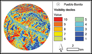
We address the computational cost of total viewshed generation on two fronts. The first involves the logic of the analytical process itself. We propose that, rather than using every cell centre of the DEM as a viewpoint, the use of a coarser grid of viewpoints over a complete study area can effectively characterise the ‘total’ visibility of a landscape, while substantially reducing processing time. Experimentation with approximately 30m-resolution elevation data for 4km-radius areas around 15 great house sites showed little to no practical difference between cumulative viewsheds produced using every cell centre as a viewpoint (for a true total viewshed) and those produced using viewpoints spaced at 5-cell (approximately 150m) intervals (Figure 1). The resulting cumulative viewsheds were standardised for comparison as proportions of the total number of viewpoints used to generate each surface, potentially yielding cell values between 0 (visible from no viewpoints) and 1 (visible from all viewpoints). The maximum values in these standardised rasters fall between about 0.2 and 0.4 (local topography severely limits the probability of any single location having a view of all or most of a study area). The maximum difference between any two surfaces was approximately 0.02, with 99 per cent of differences in cell values in all test cases falling below 0.015 (Figure 2). We consider these differences to be negligible, particularly given the generalising nature of a total viewshed approach.

Figure 1 ‘Total’ visibility surfaces for a 4km-radius study area surrounding the Andrews great house. Top: a true total viewshed, generated using every cell centre as a viewpoint; bottom: generated with viewpoints spaced at 5-cell intervals (figure by K. Dungan).
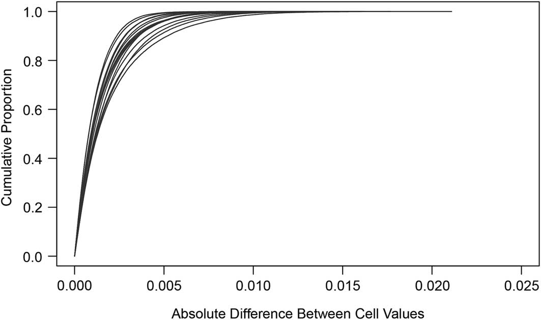
Figure 2 Cumulative distribution of the absolute differences between cell values in total viewsheds generated using 1-cell and 5-cell spacing for 15 study areas. Individual surfaces were standardised as proportions of the total number of viewpoints used to produce each total viewshed (figure by K. Dungan).
The second method to reduce computing time involves the relationship between the hardware and software used in viewshed generation and subsequent analysis of the results. Generating a single viewshed in a software package such as ArcGIS or GRASS is a time-consuming and computationally demanding process—increasingly so as the size of a DEM expands. Aggregating hundreds or thousands of viewsheds for each of the 430 sites used here would have been impractical. Devin White developed a solution to this problem by writing a viewshed algorithm in C++, a custom variant of the R2 approach (Franklin & Ray Reference Franklin and Ray1994; Osterman et al. Reference Osterman, Benedičič and Ritoša2014), converting the algorithm to a version capable of running on an NVIDIA graphics-processing unit (GPU), and optimising it to take advantage of the tens of thousands of the GPU’s small processing cores. We estimate the final algorithm to run at least 2000× faster than a similar process carried out using the legacy visibility tools in ArcGIS.
Parameters and stages of the analysis
The immediate source of the site data used here is the Chaco Social Networks (CSN) database (Peeples et al. Reference Peeples, Mills, Clark, Aragon, Giomi and Bellorado2016). The site location data were derived originally from the older Chaco World database curated at the Chaco Research Archive (http://www.chacoarchive.org/cra/outlier-database/), and were updated by the CSN Project and the Chaco Landscapes Project (Van Dyke et al. Reference Van Dyke, Lekson and Heitman2016b). Cumulatively, these initiatives have significantly improved the location data for known sites, in addition to adding new sites. The complete dataset contains point locations for 430 sites, including 269 great houses (or sites that have been recorded as great houses) and 161 non-great house sites with great kivas (Mills et al. Reference Mills, Peeples, Aragon, Bellorado, Clark, Giomi and Windes2018: fig. 1).
Defining study areas is of key importance to framing the problem of Chaco-style structure visibility in terms of local landscapes. A few great houses may have been positioned primarily to take advantage of very distinct, highly visible places within a larger landscape; Chimney Rock is probably the clearest example (Jalbert & Cameron Reference Jalbert and Cameron2000: 85–86). In general, however, potential great house locations were probably constrained by other considerations, especially convenient access to agricultural land and the actual (or potential) locations of other settlements in a local community or across the wider landscape. Our analysis relies on the assumption that, in most cases, the potential locations for any given great house were contained within a fairly restricted geographic area. In modelling proposed site territories near Mesa Verde, Varien (Reference Varien1999: 153–55, 160–65) drew on cross-cultural studies of land use to argue that a settlement’s most utilised agricultural fields would have fallen within a maximum 2km radius from the settlement itself. The assumption that settlements cluster within roughly 2km of a great house fits reasonably well with Gilpin’s (Reference Gilpin2003) suggested average great house community size of 8.3km2. Here we define local study areas—that is, the area containing potential locations for any given great house—using a 4km radius around sites, representing the 2km ‘convenience catchment’ of the great house itself, plus the 2km catchment of any sites at the edge of the great house catchment. Extending the definition of the ‘local’ landscape beyond the area immediately surrounding existing great houses allows for consideration of more distant areas used by past populations (e.g. agricultural lands) as affecting the range of potential great house locations. It should also be noted that at least some great house communities were dispersed over areas greater than Gilpin’s projected figure (e.g. Safi & Duff Reference Safi and Duff2016).
A careful consideration of the relationship of visibility to distance is critical in viewshed analysis. Even the comparatively small study areas used here will probably contain lines of sight long enough for distant elements of the landscape to lose detail and become ‘background’. As this paper focuses on location choice—which, by necessity, pre-dates the great houses or great kivas themselves—we consider views of the landscape in defining maximum visible distance rather than using great house size. We applied a 5km maximum distance for the calculation of visibility from any given viewpoint. This corresponds reasonably well with the maximum distance at which a human within the landscape might remain visible under optimal conditions, using the relationships between object size and visible distance summarised by Ogburn (Reference Ogburn2006; see also Rennel Reference Rennel2012: 516–17), and also with the proposed boundary of a middle-ground view of the landscape for regional land management (USDA Forest Service 1995: 12). The low, sparse vegetation that characterises much of the Colorado Plateau is unlikely to have significantly limited visibility across the landscape. The small proportion of the study area characterised by ponderosa pine forest, however, would have had more obstructed views. Here, we assume an adult viewer standing at ground level (i.e. with an eye height of 1.5m), sighting to the landscape at ground level.
Total viewsheds for each study area are generated using 5-cell spacing on approximately 30m resolution DEMs extracted from the ASTER satellite global DEM dataset. Each total viewshed is produced with an additional 5km buffer (i.e. the maximum visible distance) around the 4km study area. This ensures that all cells are evaluated against an equal number of viewpoints, and serves to eliminate a potential edge effect, in which cells in the outer portion of the study area are evaluated against fewer viewpoints and therefore tend to have lower values than central cells (Wheatley & Gillings Reference Wheatley and Gillings2000: 11–12) (Figure 3). The 4km-radius circular study area is extracted from this larger raster to produce the final total viewshed for each area.
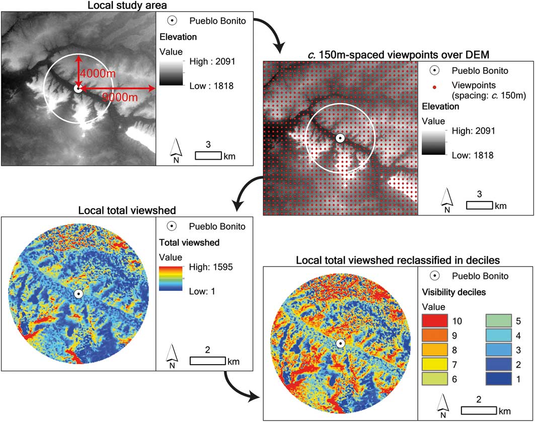
Figure 3 Schematic illustrating the steps followed in the analysis (figure by S. Déderix).
Lastly, to assess the degree to which Chaco-style architecture was positioned to take advantage of visibility afforded by the landscape, the total viewshed for each local area is classified into 10 quantiles. Therefore, the first quantile, for example, contains the 10 per cent of cells within the raster with the lowest visibility scores. To automate data production, a C++ application is used to 1) ingest a single large DEM and a shapefile with all of the sites of interest; 2) cut out a region of the DEM centred on each site with a user-specified radius; 3) execute the GPU-enabled aggregate viewshed algorithm with a maximum viewable distance applied; 4) apply a circular mask to the results based on a user-specified radius; and 5) reclassify the unmasked data into deciles. The software is not currently available for public distribution, but a very similar result can be achieved via Python scripting and the GPU-enabled ‘Viewshed 2’ tool in ArcMap. In order to compensate for potential inaccuracy in site location data, visibility scores for individual structures are calculated as the mean decile value (rounded to the nearest whole number) for the 3-cell neighbourhood surrounding the structure point location. The distribution of site-visibility values can then be evaluated against the background landscape distribution.
Results and discussion
The results clearly show that great houses are unevenly distributed among visibility deciles, with approximately half of the great houses falling into the eighth decile or higher (Figures 4–6) (Table S1). This pattern is most obvious for great houses built after c. AD 1000. This may be due in part to sample size: the majority of great house construction dates to the eleventh-century florescence of the Chaco World, although a substantial proportion of the smaller count of twelfth-century great houses falls within the highest decile. There does, however, appear to be some preference for higher visibility deciles among earlier great houses.

Figure 4 Histograms showing the distribution of great houses and great kiva sites within visibility deciles (figure by K. Dungan).
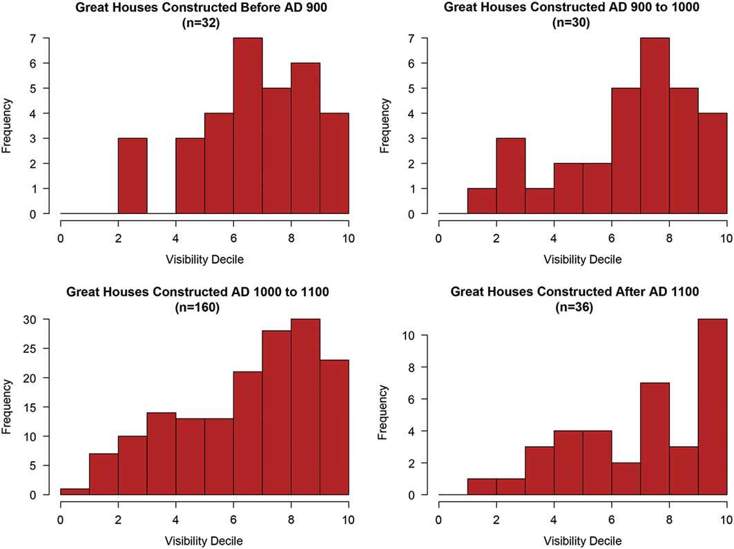
Figure 5 Histograms showing the distribution of great houses within visibility deciles by construction date (figure by K. Dungan).
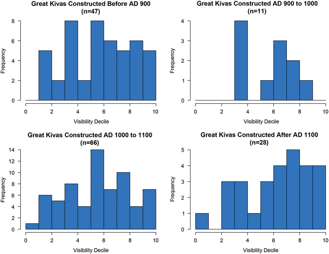
Figure 6 Histograms showing the distribution of great kiva sites within visibility deciles by construction date (figure by K. Dungan).
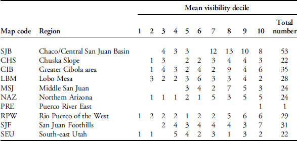
Applying a Kolmogorov-Smirnov (K-S) statistical test suggests that the great house distribution within visibility deciles differs significantly from the uniform distribution of visibility deciles on the landscape, both when great houses are considered as a single group and when they are grouped by century of construction (Figure 7 & Table 1). In addition, great house visibility shows relatively little geographic variation. The preference for higher visibility deciles seems to be present in areas at the edges of the larger study area, as well as in Chaco Canyon and the central San Juan Basin (Reference Hayes and WindesFigure 8 & Table 2). Two groups of sites stand out for their lack of emphasis on high visibility: these are the great houses in the far northern portion of the study area, particularly south-eastern Utah, and those at the southern edge of the San Juan Basin near Lobo Mesa, including the Red Mesa Valley.
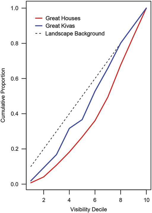
Figure 7 The distribution of great house and great kiva sites by visibility decile, plotted as cumulative proportions against the uniform background distribution (figure by K. Dungan).
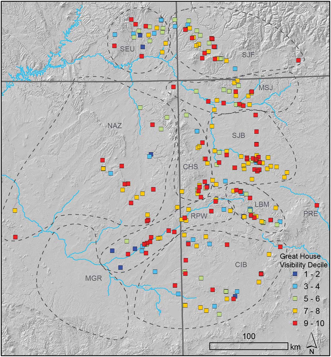
Figure 8 Great house sites included in the study, showing visibility deciles and regional grouping (dashed areas, see Table 2) (figure by K. Dungan).
Table 1 The results of Kolmogorov-Smirnov tests applied to the distribution within visibility deciles of great houses against background values, great kivas against background values, great houses against great kivas, and Silver Creek/Mogollon Rim great kivas against all other great kivas. Two distributions can be said to differ at a given level of significance (α) if the maximum observed difference (Max D) between the two cumulative distributions exceeds the critical value for that significance level. The calculation of significance levels against a very large background population (*) is described in Kvamme (Reference Kvamme1990: 369–70). The number of great kivas dating to the tenth century was insufficient to justify statistical testing for this interval.
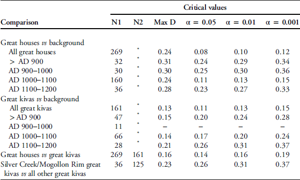
Table 2 Great house counts within visibility deciles grouped by region (see map in Figure 8).
In contrast to the great houses, great kiva sites show much more frequent use of moderate or lower-visibility site locations—a pattern that remains consistent over time. K-S tests suggest that the distribution of great kivas within visibility deciles differs significantly from the uniform background distribution when all great kivas are grouped together, but not when the sites are grouped by presumed construction date (although the resulting sample sizes are small). Yet is it reasonable to expect archaeological sites to be uniformly distributed among visibility deciles? Very few sites of either category fall within the lowest decile, and it is possible that topographic factors that shape locational visibility may also affect suitability as a building site; that is, very low visibility areas (e.g. near drainages) may be unsuitable for construction. Regardless, a comparison of the great kiva and great house distributions using a K-S test supports the proposition that the two differ significantly.
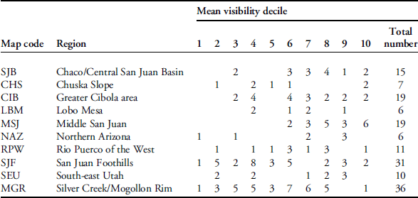
Great kiva visibility seems to be largely consistent across the study area. This is of particular interest, given the inclusion in the study of the great kiva sites around Silver Creek and the Mogollon Rim in east-central Arizona (Reference Jalbert and CameronFigure 9 & Table 3). No great houses were built in this region, and many of the great kivas appear to have been unroofed, making the inclusion of these sites in the ‘Chaco World’ somewhat debatable. Despite this, the pattern of visibility seen in these great kivas does not differ meaningfully from that present in great kivas in more clearly ‘Chacoan’ areas. One subregion that may show an unusual emphasis on great kiva visibility is the Middle San Juan, where approximately half of the great kivas fall into the two uppermost visibility deciles.
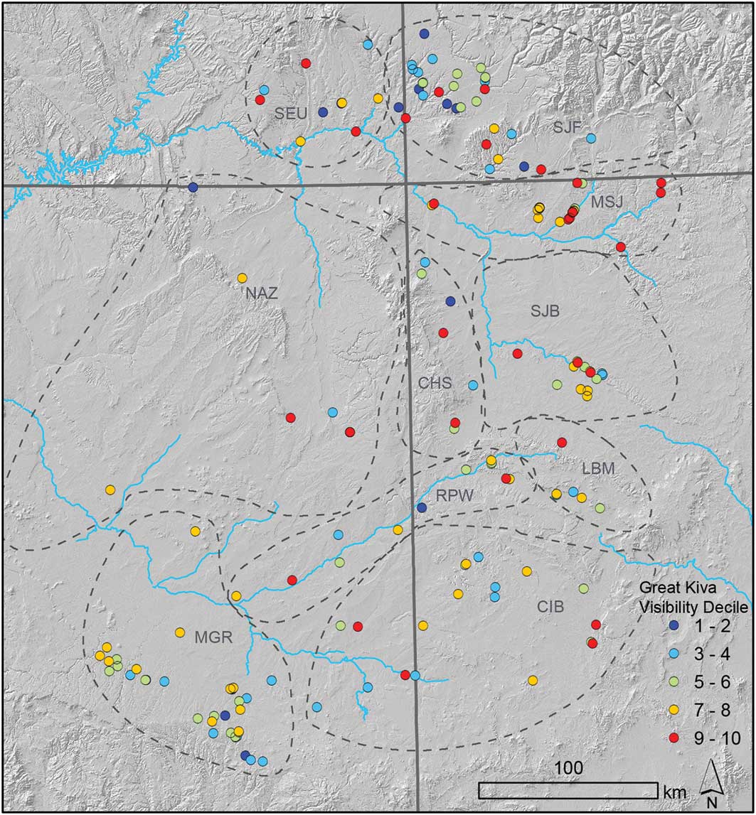
Figure 9 Great kiva sites included in the study, showing visibility deciles and regional grouping (dashed areas, see Table 3) (figure by K. Dungan).
Table 3 Great kiva counts within visibility deciles grouped by region (see map in Figure 9).
The results described above suggest a broad pattern of difference in site placement between great houses and great kivas. It is probable that great house locations were often chosen to take advantage of the visibility afforded by local landscapes, while great kivas were much less likely to have been placed with a concern for visibility—even if they rarely utilised the least visible portions of the landscape. Notably, these differences fit with the visibility afforded by great house and great kiva architecture. Both types of structures are defined by size, degree of planning and what might be considered ‘overbuilding’ (i.e. construction that is more formal, massive or labour-intensive than is strictly necessary; Stein & Lekson Reference Stein and Lekson1992). But while great house design could be expanded through the addition of further rooms or floors, the maximum size of great kivas—as single, usually roofed rooms—was much more constrained. As the largest indoor spaces in the ancient Southwest, great kivas were certainly of a scale intended to impress, but this monumentality was primarily experienced from within the structure. In contrast, great houses are inherently more visible from a distance. We suggest that this inherent ‘legibility’ (sensu Moore Reference Moore1996: 97) was frequently enhanced through the choice of setting; great houses were intended to be seen by individuals across the wider landscape, rather than only by viewers in the immediate vicinity of the building.
This pattern may also speak to discussions of travel to great houses over greater distances, such as during pilgrimage (e.g. Van Dyke Reference Van Dyke2007a). The choice of highly visible locations may have allowed great houses to serve as landmarks for, and to make an impression on, visitors entering a community. The differing purposes of great kivas and great houses are also worth noting. While the former were constructed as communal religious venues, great houses served, at least to some extent, as dwellings; the selection of highly visible building sites was probably tied to the display of power by the residents of great houses. Moreover, the fact that great kivas are characterised by a lack of concern for visibility suggests that, despite being an expressly religious or public form of architecture, they may not have conveyed a Chacoan ideology in the same way as great houses.
This analysis has aimed to explore potential commonalities in visibility across the wider Chaco World. The resulting data, however, should also be valuable for the examination of visibility at local scales and in relationship to local histories and geography. For example, the area around Lobo Mesa—a subregion that stands out from the larger analysis as having a higher proportion of great houses in less visible locations—is characterised by the early use of great houses, particularly in the Red Mesa Valley (Van Dyke Reference Van Dyke2000). Unlike later great houses in the same area, these early examples (such as the Andrews great house) do seem frequently to have been placed in high visibility locations. It is possible that existing land tenure constrained the placement of later great houses, which were built in locations with more modest visibility, despite the emphasis on high visibility that characterises the eleventh-century peak of great house construction across the larger study area. These later great houses include the two sites with tower kivas that Kantner and Hobgood (Reference Kantner and Hobgood2016) argue were intended to be viewed locally. Notably, the location of neither great house falls within a high visibility decile (they fall in the fifth and sixth deciles); potentially, the towers compensated for the moderate visibility afforded by the building sites. A detailed exploration of visibility at the subregional scale is beyond the scope of this article, but it is valuable to note the presence of geographic diversity within larger patterns of great house and great kiva use.
Conclusion
This study illustrates the utility of a modified total viewshed approach in addressing site placement, and demonstrates the degree to which the development of software that fully utilises advances in hardware can make this computationally intensive technique practical. The essential method applied here can be replicated with other software packages, and the use of expanded viewpoint spacing should reduce analytical time, regardless of the platform used.
While sight can be presumed to be critical in experiencing monumental architecture, it does not necessarily follow that monumental constructions were placed within the landscape to be highly visible. Some British prehistoric stone circles, for example, may have been placed to constrain their viewsheds, or limit how they could be viewed (Bradley Reference Bradley2002: 75; Lake & Ortega Reference Lake and Ortega2013). Visibility is only one element of our wider understanding of Chaco, but, as few ‘outlying’ great houses and great kivas have been excavated relative to the large number of proposed Chaco communities, architectural surface remains and site placement are critical variables for examining diversity in the Chaco World. Based on the results presented here, we argue that the overbuilding that defines great houses was frequently enhanced by the selection of highly visible building sites, while visibility was less of a concern in great kiva placement. This probably speaks to the physical differences between the two forms of architecture—great houses are inherently better suited for visibility at a distance—but may also be tied to differing social roles, with great houses displaying the power of their builders and residents. These patterns apparently persist through time and are certainly evident by the eleventh-century AD peak of great house construction (see Mills et al. Reference Mills, Peeples, Aragon, Bellorado, Clark, Giomi and Windes2018). We suggest that, among the ideological components that unite the Chaco World, there was a tradition of landscape use intended to enhance the visibility of great houses—and whatever meanings they conveyed or reactions they evoked—to an audience living within or moving through local landscapes. A concern with ‘being seen’ is a fundamental part of the story of Chaco-style architecture.
Acknowledgements
The Chaco Social Networks (CSN) project was funded through the National Science Foundation (grant numbers 1355381 (PI Jeffery Clark, Archaeology Southwest) and 1355374 (PI Barbara Mills, University of Arizona)). We are grateful to our CSN colleagues for their feedback and assistance, to the Chaco Research Archive and the Chaco Landscapes Project for making site data available, and to two anonymous reviewers for their helpful comments. This research was supported by a SPARC Award. The SPARC Program is based at the Center for Advanced Spatial Technologies at the University of Arkansas and is funded by the National Science Foundation (awards 1321443 and 1519660). The ASTER Global Digital Elevation Model is a product of NASA and the Ministry of Economy, Trade, and Industry of Japan.
Supplementary material
To view supplementary material for this article, please visit https://doi.org/10.15184/aqy.2018.135


