1. Introduction
Faraday rotation provides a mechanism for probing magnetic fields in both the nearby and distant Universe on a range of physical and spatial scales (Johnston-Hollitt et al. Reference Johnston-Hollitt2015). In Faraday rotation the angle of linearly polarised light rotates as a function of wavelength as it passes through an ionic magnetised medium. By using polarised sources as backlights, we can constrain magnetic fields in a host of environments including the interstellar and intracluster media, and potentially even the elusive cosmic web (Johnston-Hollitt et al. Reference Johnston-Hollitt2015). Faraday rotation is thus vital to understanding the role of magnetic fields in the Universe.
Multiple methods have been developed to characterise the frequency dependent structure seen in spectropolarimetric observations and thereby extract information on Faraday rotation, with the most popular approaches currently being rotation measure (RM) synthesis (Burn Reference Burn1966; Brentjens & de Bruyn Reference Brentjens and de Bruyn2005) and non-linear parametric fitting (i.e. QU-fitting) (e.g. Anderson, Gaensler, & Feain Reference Anderson, Gaensler and Feain2016). RMCLEAN is a CLEAN algorithm (Heald, Braun, & Edmonds Reference Heald, Braun and Edmonds2009) that is typically used to deconvolve the RM synthesis signal. Recent studies that use these methods to study the complexity of a Faraday rotated signal include Farnsworth et al. (Reference Farnsworth, Rudnick and Brown2011), O’Sullivan et al. (Reference O’Sullivan2012), Ideguchi et al. (Reference Ideguchi, Takahashi, Akahori, Kumazaki and Ryu2014), Kumazaki et al. (Reference Kumazaki, Akahori, Ideguchi, Kurayama and Takahashi2014), Sun et al. (Reference Sun2015), Pasetto et al. (Reference Pasetto, Carrasco-GonzÁlez, O’Sullivan, Basu, Bruni, Kraus, Curiel and Mack2018), Miyashita et al. (Reference Miyashita, Ideguchi, Nakagawa, Akahori and Takahashi2018), Thomson et al. (Reference Thomson2021). Each method is limited by the range and number of observed wavelengths. For previous generations of radio telescopes, observations of the emitting source have often been limited to narrow bands. However, as next-generation radio telescopes telescopes such as the Murchison Widefield Array (MWA; Wayth et al. Reference Wayth2018; Riseley et al. Reference Riseley2018; Riseley et al. Reference Riseley2020), the Low Frequency Array (LOFAR; van Haarlem et al. Reference van Haarlem2013; Van Eck et al. Reference Van Eck2018), the Australian Square Kilometre Array Pathfinder (ASKAP; Johnston et al. Reference Johnston2007), and MeerKAT (Jonas 2009) observe the polarised radio sky, there is a new opportunity to constrain magnetic field models in the Universe at unprecedented precision. This has led to consideration of what method works best to determine the correct RM structure from polarised spectra. With the exception of non-linear parametric QU-fitting, most RM acquisition methods are not built for the broadband context. For example, until recently channel depolarisation at low frequencies was not corrected for limiting the bands over which polarised signals could be analysed (Pratley & Johnston-Hollitt Reference Pratley and Johnston-Hollitt2020), for example, for telescopes such as the MWA. Broadband observations and fitting methods are needed for astronomers to have access to complex Faraday structures that are currently not either observed or understood.
In this work, we highlight a largely ignored but critical challenge when fitting broadband spectra in Faraday depth. When fitting a sinusoidal model along an axis in which we are using only measuring data collected from a region along the x-axis for which
 $x \geq 0$
, the nature of the sinusoidal signal implies the model will also be extendable to regions that have
$x \geq 0$
, the nature of the sinusoidal signal implies the model will also be extendable to regions that have
 $x \leq 0$
. In the case of Faraday rotation where we are fitting flux densities in
$x \leq 0$
. In the case of Faraday rotation where we are fitting flux densities in
 $\lambda^2$
space, where
$\lambda^2$
space, where
 $\lambda$
is the wavelength of light, we are performing a fit over values collected for
$\lambda$
is the wavelength of light, we are performing a fit over values collected for
 $\lambda^2 > 0$
. This implies the flux density values for
$\lambda^2 > 0$
. This implies the flux density values for
 $\lambda^2 \leq 0$
, are typically not constrained in a fitted Faraday depth model.
$\lambda^2 \leq 0$
, are typically not constrained in a fitted Faraday depth model.
However, the flux contributions for
 $\lambda^2 \leq 0$
can change the structures seen in the Faraday spectrum of the fitted solution. Using both simulated and real observations, we show empirically that it is possible to prevent introducing these structures in model fitting by constraining the flux to be 0 for
$\lambda^2 \leq 0$
can change the structures seen in the Faraday spectrum of the fitted solution. Using both simulated and real observations, we show empirically that it is possible to prevent introducing these structures in model fitting by constraining the flux to be 0 for
 $\lambda^2 \leq 0$
, such that the fitted model is not determined by non-observable flux at
$\lambda^2 \leq 0$
, such that the fitted model is not determined by non-observable flux at
 $\lambda^2 \leq 0$
. We show that this suppresses structures that cannot be observed due to their fitted flux originating over
$\lambda^2 \leq 0$
. We show that this suppresses structures that cannot be observed due to their fitted flux originating over
 $\lambda^2 \leq 0$
but otherwise will contribute to the Faraday spectrum. We emphasise that finding a
$\lambda^2 \leq 0$
but otherwise will contribute to the Faraday spectrum. We emphasise that finding a
 $\lambda^2 \leq 0$
constrained solution has only been made possible using recent convex optimisation algorithms that can include non-continuous and non-differentiable constraints and the use of RMCLEAN-like sparsity priors, for example, the primal-dual based algorithm used in this work Combettes et al. (Reference Combettes, Condat, Pesquet and Vu2014) and the alternating direction method of multipliers (ADMM) algorithm used in Pratley & Johnston-Hollitt (Reference Pratley and Johnston-Hollitt2020).
$\lambda^2 \leq 0$
constrained solution has only been made possible using recent convex optimisation algorithms that can include non-continuous and non-differentiable constraints and the use of RMCLEAN-like sparsity priors, for example, the primal-dual based algorithm used in this work Combettes et al. (Reference Combettes, Condat, Pesquet and Vu2014) and the alternating direction method of multipliers (ADMM) algorithm used in Pratley & Johnston-Hollitt (Reference Pratley and Johnston-Hollitt2020).
This work starts by introducing the Faraday RM synthesis measurement equation in Section 2. We then discuss the aspects of flux densities for
 $\lambda^2 \leq 0$
and the implications in Section 3. In Section 4 we introduce the minimisation problem that can reconstruct a Faraday rotation signal and not include the non-observable flux density in the Faraday spectrum. We demonstrate the impact of removing this flux density in signal reconstruction in Section 5. We conclude that this work is important for Faraday analysis with non-parametric reconstruction algorithms like CLEAN in Section 6.
$\lambda^2 \leq 0$
and the implications in Section 3. In Section 4 we introduce the minimisation problem that can reconstruct a Faraday rotation signal and not include the non-observable flux density in the Faraday spectrum. We demonstrate the impact of removing this flux density in signal reconstruction in Section 5. We conclude that this work is important for Faraday analysis with non-parametric reconstruction algorithms like CLEAN in Section 6.
2. Faraday synthesis measurement equation
The relation between the coordinates of the Faraday spectrum, Faraday depth
 $\phi$
, and
$\phi$
, and
 $\lambda^2$
is given by the measurement equation
$\lambda^2$
is given by the measurement equation
 \begin{equation} w_{k}P(\lambda^2_k) = \int_{-\infty}^{\infty} w_{k}a(\delta\lambda^2_k, \phi)F(\phi) {\rm e}^{2i\lambda^2_k\phi} {\rm d}\phi + w_{k}n(\lambda^2_k)\, ,\end{equation}
where P is the complex valued linear polarisation, F is the Faraday spectrum, n is the noise,
 $w_k$
are weights that can be used to account for uncertainty while assuming no noise co-variance, and for a limited range of
$w_k$
are weights that can be used to account for uncertainty while assuming no noise co-variance, and for a limited range of
 $\lambda^2_k$
values and channel widths
$\lambda^2_k$
values and channel widths
 $\delta \lambda^2_k$
; we are limited in both
$\delta \lambda^2_k$
; we are limited in both
 $\phi$
values and Faraday resolution
$\phi$
values and Faraday resolution
 $\delta \phi$
(Burn Reference Burn1966; Brentjens & de Bruyn Reference Brentjens and de Bruyn2005; Pratley & Johnston-Hollitt Reference Pratley and Johnston-Hollitt2020). As discussed by Pratley & Johnston-Hollitt (Reference Pratley and Johnston-Hollitt2020), we can model the impact of channel averaging by including a channel dependent sensitivity window in Faraday depth
$\delta \phi$
(Burn Reference Burn1966; Brentjens & de Bruyn Reference Brentjens and de Bruyn2005; Pratley & Johnston-Hollitt Reference Pratley and Johnston-Hollitt2020). As discussed by Pratley & Johnston-Hollitt (Reference Pratley and Johnston-Hollitt2020), we can model the impact of channel averaging by including a channel dependent sensitivity window in Faraday depth
 $a(\delta\lambda^2_k, \phi)$
, this is also known as the
$a(\delta\lambda^2_k, \phi)$
, this is also known as the
 $\delta\lambda^2$
-projection term and it is useful at long wavelengths. While Pratley & Johnston-Hollitt (Reference Pratley and Johnston-Hollitt2020) uses channel averaging in
$\delta\lambda^2$
-projection term and it is useful at long wavelengths. While Pratley & Johnston-Hollitt (Reference Pratley and Johnston-Hollitt2020) uses channel averaging in
 $\lambda^2$
as an example, the averaging process is always linear by definition and different window sensitivity functions are possible, for example, Schnitzeler & Lee (Reference Schnitzeler and Lee2017) who considered channel averaging in
$\lambda^2$
as an example, the averaging process is always linear by definition and different window sensitivity functions are possible, for example, Schnitzeler & Lee (Reference Schnitzeler and Lee2017) who considered channel averaging in
 $\nu$
. For bandlimited functions, there is an exact Fourier series relation between
$\nu$
. For bandlimited functions, there is an exact Fourier series relation between
 $\textbf{y}_k = P(\lambda^2_k)$
and
$\textbf{y}_k = P(\lambda^2_k)$
and
 $\textbf{x}_l = F(\phi_l)$
after including additive noise
$\textbf{x}_l = F(\phi_l)$
after including additive noise
 $\textbf{n}_k = n(\lambda^2_k)$
. We can write this relation as the matrix equation
$\textbf{n}_k = n(\lambda^2_k)$
. We can write this relation as the matrix equation
 $${\bf{Wy}} = \Phi {\bf{x}} + {\rm{ }}{\bf{Wn}}{\mkern 1mu} ,$$
where
 $\textbf{x}\in \mathbb{C}^N$
and
$\textbf{x}\in \mathbb{C}^N$
and
 $\textbf{y}, \textbf{n}\in \mathbb{C}^M$
, and where the measurement matrix
$\textbf{y}, \textbf{n}\in \mathbb{C}^M$
, and where the measurement matrix
 ${\boldsymbol{\Phi}} \in \mathbb{C}^{M \times N}$
is defined as
${\boldsymbol{\Phi}} \in \mathbb{C}^{M \times N}$
is defined as
 \begin{equation} {\boldsymbol{\Phi}}_{kl} = w_{k}a(\delta\lambda^2_k, \phi_l){\rm e}^{2i\lambda^2_k\phi_l}\, ,\end{equation}
and the diagonal weighting matrix is
 $\textbf{W}_{kk} = w_k$
. For many cases, like the examples in this paper, we can store
$\textbf{W}_{kk} = w_k$
. For many cases, like the examples in this paper, we can store
 ${\boldsymbol{\Phi}}$
as a matrix.
${\boldsymbol{\Phi}}$
as a matrix.
3. Non-Observable Structure in Models of Broadband Emission
In this section, we discuss non-observable contributions of flux in the fitted model. For example, we expect that
 $P(\lambda^2 = 0) = 0$
due to the measured flux decreasing as
$P(\lambda^2 = 0) = 0$
due to the measured flux decreasing as
 $\nu \equiv c/\lambda \to \infty$
. In general, the population of photons decreases to zero as energy increases.Footnote
1
There is a more philosophical question about flux for
$\nu \equiv c/\lambda \to \infty$
. In general, the population of photons decreases to zero as energy increases.Footnote
1
There is a more philosophical question about flux for
 $\lambda^2 \leq 0$
. Since imaginary
$\lambda^2 \leq 0$
. Since imaginary
 $i\lambda$
wavelengths do not exist, this flux corresponds to the observed Faraday rotation if it was in the opposite sense, that is, all magnetic fields are reversed (Burn Reference Burn1966). We cannot observe the energy for this signal unless this energy is shifted to positive
$i\lambda$
wavelengths do not exist, this flux corresponds to the observed Faraday rotation if it was in the opposite sense, that is, all magnetic fields are reversed (Burn Reference Burn1966). We cannot observe the energy for this signal unless this energy is shifted to positive
 $\lambda^2$
, for example, through helicity (Brandenburg & Stepanov Reference Brandenburg and Stepanov2014; Horellou & Fletcher Reference Horellou and Fletcher2014). We suggest that a reconstructed Faraday spectrum therefore should not have contributing flux over the
$\lambda^2$
, for example, through helicity (Brandenburg & Stepanov Reference Brandenburg and Stepanov2014; Horellou & Fletcher Reference Horellou and Fletcher2014). We suggest that a reconstructed Faraday spectrum therefore should not have contributing flux over the
 $\lambda^2 \leq 0$
half of the domain.
$\lambda^2 \leq 0$
half of the domain.
Even in the case where we use conjugate symmetry to determine the flux for the negative
 $\lambda^2$
, it is determined by the flux for positive
$\lambda^2$
, it is determined by the flux for positive
 $\lambda^2$
. The negative
$\lambda^2$
. The negative
 $\lambda^2$
flux will be a factor for distinguishing and constraining Galactic magnetic field models for each line of sight component, for example, such modelling may be accomplished by the Interstellar MAGnetic field INference Engine (IMAGINE; Boulanger et al. Reference Boulanger2018), which will perform a full Bayesian analysis of currently available polarimetric data. There are physical Faraday spectra, as suggested by Brandenburg & Stepanov (Reference Brandenburg and Stepanov2014), which will not be consistent with conjugate symmetry in
$\lambda^2$
flux will be a factor for distinguishing and constraining Galactic magnetic field models for each line of sight component, for example, such modelling may be accomplished by the Interstellar MAGnetic field INference Engine (IMAGINE; Boulanger et al. Reference Boulanger2018), which will perform a full Bayesian analysis of currently available polarimetric data. There are physical Faraday spectra, as suggested by Brandenburg & Stepanov (Reference Brandenburg and Stepanov2014), which will not be consistent with conjugate symmetry in
 $\lambda^2 \leq 0$
. This emphasises that every model Faraday spectrum should be filtered to contain only
$\lambda^2 \leq 0$
. This emphasises that every model Faraday spectrum should be filtered to contain only
 $\lambda^2 > 0$
flux before comparing with observation. This leaves many models that are equivalent only after observable information is considered.
$\lambda^2 > 0$
flux before comparing with observation. This leaves many models that are equivalent only after observable information is considered.
Restricting to
 $\lambda^2 > 0$
has implications for the analysis of the Faraday spectra, which we will briefly cover. The linear polarisation P is related to the total intensity I through
$\lambda^2 > 0$
has implications for the analysis of the Faraday spectra, which we will briefly cover. The linear polarisation P is related to the total intensity I through
 \begin{equation} P(\nu) = I(\nu) p(\nu)\, ,\end{equation}
where
 $p(\nu)$
is the complex fractional linear polarisation, and
$p(\nu)$
is the complex fractional linear polarisation, and
 $|p| \leq 1$
.Footnote
2
It follows that, after a change of variables, we have the relation
$|p| \leq 1$
.Footnote
2
It follows that, after a change of variables, we have the relation
 \begin{equation} P(\lambda^2) = I(\lambda^2) p(\lambda^2)\, ,\end{equation}
and it follows from the convolution theorem that
 \begin{equation} F(\phi)= (K \star f)(\phi)\, . \end{equation}
In the above we have assumed an ideal Fourier relation with
 \begin{equation} I(\lambda^2) = \int_{-\infty}^{\infty} K(\phi) {\rm e}^{2i\lambda^2\phi}\, {\rm d}\phi\, .\end{equation}
The Faraday depth coordinate
 $\phi$
for K represents a pseudo Faraday depth component that is purely due to the spectral structure and structure of
$\phi$
for K represents a pseudo Faraday depth component that is purely due to the spectral structure and structure of
 $I(\lambda^2)$
that mimics Faraday rotation modesFootnote
3
and f is the Faraday rotation spectrum of p. We define spectral structure as structure of the spectrum in
$I(\lambda^2)$
that mimics Faraday rotation modesFootnote
3
and f is the Faraday rotation spectrum of p. We define spectral structure as structure of the spectrum in
 $|P(\lambda^2)|$
, which is typically determined by
$|P(\lambda^2)|$
, which is typically determined by
 $I(\lambda^2)$
. This spectral structure over broad bandwidths creates an intrinsic broadening of the RM component
$I(\lambda^2)$
. This spectral structure over broad bandwidths creates an intrinsic broadening of the RM component
 $\phi_0$
, though we expect for many cases the resolution limit determined by the limited
$\phi_0$
, though we expect for many cases the resolution limit determined by the limited
 $\lambda^2$
coverage is far too coarse to observe this.Footnote
4
$\lambda^2$
coverage is far too coarse to observe this.Footnote
4
We now introduce the Heaviside step function as
 $\Theta(\lambda^2) = 0$
for
$\Theta(\lambda^2) = 0$
for
 $\lambda^2 \leq 0$
and
$\lambda^2 \leq 0$
and
 $\Theta(\lambda^2) = 1$
otherwise. The value at
$\Theta(\lambda^2) = 1$
otherwise. The value at
 $\Theta(0) = 1$
typically has no impact on its integration. The positive
$\Theta(0) = 1$
typically has no impact on its integration. The positive
 $\lambda^2$
linear polarisation signal reads
$\lambda^2$
linear polarisation signal reads
 \begin{equation} P_{\lambda^2 > 0}(\lambda^2) = \Theta(\lambda^2)I(\lambda^2) p(\lambda^2)\, , \end{equation}
with
 $P_{\lambda^2 \leq 0}(\lambda^2) = P(\lambda^2) - P_{\lambda^2 > 0}(\lambda^2)$
. We then have the relation
$P_{\lambda^2 \leq 0}(\lambda^2) = P(\lambda^2) - P_{\lambda^2 > 0}(\lambda^2)$
. We then have the relation
 \begin{equation} F_{\lambda^2 > 0}(\phi) = \frac{\pi}{2i}H[F](\phi) + \frac{1}{2}F(\phi)\, , \end{equation}
where H[F] is the Hilbert transform of
 $F(\phi)$
, defined as
$F(\phi)$
, defined as
 \begin{equation} H[F](\phi) = \frac{1}{\pi}\int_{-\infty}^\infty \frac{F(\phi^\prime)}{\phi - \phi^\prime}\, {\rm d}\phi^\prime\, ,\end{equation}
which in some cases has a closed form expression. We calculate the fractional polarisation without any spectral structure from total intensity I as
 \begin{equation} p_{\lambda^2 > 0}(\lambda^2) = \Theta(\lambda^2)p(\lambda^2)\, ,\end{equation}
and
 \begin{equation} f_{\lambda^2 > 0}(\phi) = \frac{\pi}{2i}H[f](\phi) + \frac{1}{2}f(\phi)\, .\end{equation}
The Hilbert transform is also encountered in all sky interferometric imaging, and there is a natural analogy between the two contexts. In Equation (27) of Pratley et al. (Reference Pratley, Johnston-Hollitt and McEwen2019), the Hilbert transform could be used in the uvw-domain to restrict an all sky signal to be above the horizon. This is analogous to restricting a spectro-polarmetric signal to positive
 $\lambda^2$
. However, unlike interferometric imaging where we can use multiple observations to get full sky coverage, we cannot build a telescope to observe and constrain negative
$\lambda^2$
. However, unlike interferometric imaging where we can use multiple observations to get full sky coverage, we cannot build a telescope to observe and constrain negative
 $\lambda^2$
.
$\lambda^2$
.
A common model for Faraday rotation with many components is the Burn slab
 $\Pi_{[\phi_a, \phi_b]}(\phi)$
, where
$\Pi_{[\phi_a, \phi_b]}(\phi)$
, where
 $\Pi_{[\phi_a, \phi_b]}(\phi) = 1$
for
$\Pi_{[\phi_a, \phi_b]}(\phi) = 1$
for
 $\phi \in [\phi_a, \phi_b]$
and
$\phi \in [\phi_a, \phi_b]$
and
 $\Pi_{[\phi_a, \phi_b]}(\phi) = 0$
otherwise (Burn Reference Burn1966). The Faraday spectrum after removing non-observable structure from
$\Pi_{[\phi_a, \phi_b]}(\phi) = 0$
otherwise (Burn Reference Burn1966). The Faraday spectrum after removing non-observable structure from
 $\lambda^2 \leq 0$
for
$\lambda^2 \leq 0$
for
 $f(\phi) = \Pi_{[\phi_a, \phi_b]}(\phi)$
is
$f(\phi) = \Pi_{[\phi_a, \phi_b]}(\phi)$
is
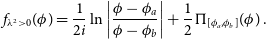 \begin{equation} f_{\lambda^2 > 0}(\phi) = \frac{1}{2i}\ln{\left|\frac{\phi - \phi_a}{\phi - \phi_b}\right|} + \frac{1}{2}\Pi_{[\phi_a, \phi_b]}(\phi)\, .\end{equation}
We can remove non-observable structure from
 $\lambda^2 \leq 0$
from a Faraday thin component
$\lambda^2 \leq 0$
from a Faraday thin component
 $f(\phi) = \delta(\phi - \phi_0)$
centred at
$f(\phi) = \delta(\phi - \phi_0)$
centred at
 $\phi_0$
to read
$\phi_0$
to read
 \begin{equation} f_{\lambda^2 > 0}(\phi) = \frac{1}{2i (\phi - \phi_0)} + \frac{1}{2}\delta(\phi - \phi_0)\, .\end{equation}
We can repeat the same calculations for spectral structure due to total intensity to find similar functional forms (see Figure 1).
Figure 1. Real and imaginary parts for a Burn slab with the interval
 $\pm 10$
rad m-2 (left) and for a Faraday thin screen located at 0 rad m-2 (right) in Faraday depth for
$\pm 10$
rad m-2 (left) and for a Faraday thin screen located at 0 rad m-2 (right) in Faraday depth for
 $f_{\lambda^2 > 0}(\phi)$
. These models only contain flux over positive
$f_{\lambda^2 > 0}(\phi)$
. These models only contain flux over positive
 $\lambda^2$
.
$\lambda^2$
.
New broadband surveys like Polarisation Sky Survey of the Universe’s Magnetism (POSSUM; Gaensler et al. Reference Gaensler, Landecker and Taylor2010), Very Large Array Sky Survey (VLASS; Lacy et al. Reference Lacy2020), and QU Observations at Cm wavelength with Km baselines using ATCA (QUOCKAFootnote
5
) have the opportunity to measure and fit more complex Faraday structure in Faraday depth. However, the fitted complex Faraday structures should only include flux from positive
 $\lambda^2$
. In the next section we discuss how this can be done from a fitting perspective.
$\lambda^2$
. In the next section we discuss how this can be done from a fitting perspective.
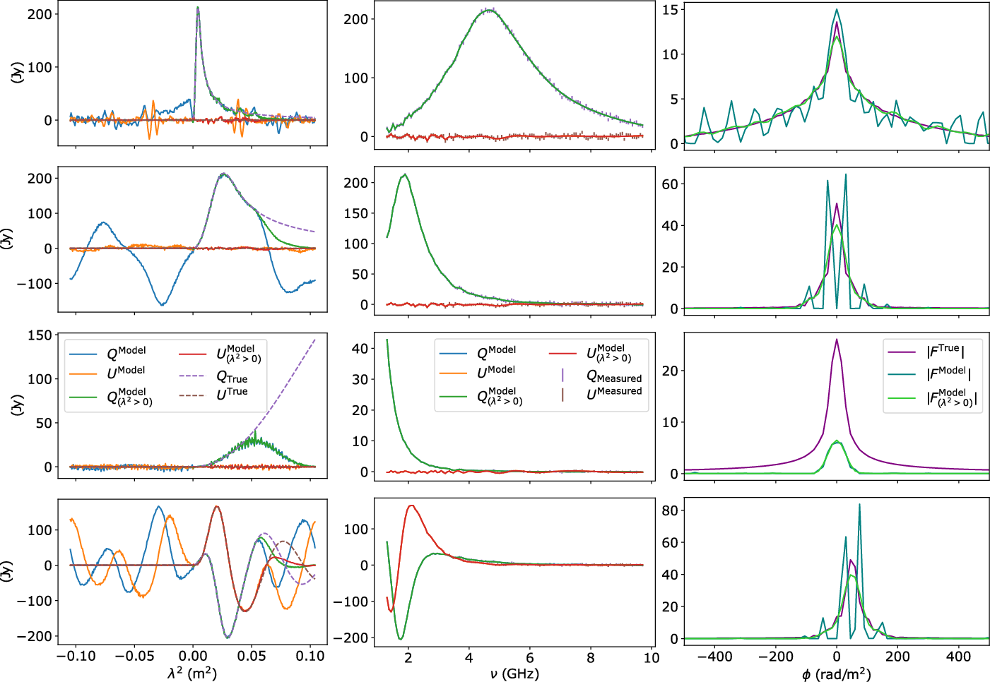
Figure 2. Reconstructions of simulated synchrotron spectra
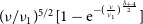 $(\nu/\nu_1)^{5/2}[1 - {\rm e}^{-(\frac{\nu}{\nu_1})^{\frac{\delta + 4}{2}}} ]$
, where
$(\nu/\nu_1)^{5/2}[1 - {\rm e}^{-(\frac{\nu}{\nu_1})^{\frac{\delta + 4}{2}}} ]$
, where
 $\delta$
is the power law slope for the energy spectrum of cosmic-ray electrons, using a CLEAN style prior in Faraday depth, with and without the prior of
$\delta$
is the power law slope for the energy spectrum of cosmic-ray electrons, using a CLEAN style prior in Faraday depth, with and without the prior of
 $P_{\lambda^2 \leq 0}(\lambda^2) = 0$
. Rows 1, 2, 3, and 4 have breaking frequencies
$P_{\lambda^2 \leq 0}(\lambda^2) = 0$
. Rows 1, 2, 3, and 4 have breaking frequencies
 $\nu_1 = 800, 2\,000, 5\,000, 2\,000$
MHz respectively with a spectral index of
$\nu_1 = 800, 2\,000, 5\,000, 2\,000$
MHz respectively with a spectral index of
 $\alpha \equiv -(\delta - 1)/2 = -0.8$
. Rows 1–3 have no rotation measure, and row 4 has a component at 100 rad m-2. Column 1 shows
$\alpha \equiv -(\delta - 1)/2 = -0.8$
. Rows 1–3 have no rotation measure, and row 4 has a component at 100 rad m-2. Column 1 shows
 $Q(\lambda^2)$
and
$Q(\lambda^2)$
and
 $U(\lambda^2)$
for the reconstructed model both with and without the prior, and the ground truth. Column 2 compares the fit over the observed
$U(\lambda^2)$
for the reconstructed model both with and without the prior, and the ground truth. Column 2 compares the fit over the observed
 $\nu$
range. Column 3 compares the absolute values of the ground truth and reconstructed Faraday depth signals. Significant spectral structure can introduce structure in
$\nu$
range. Column 3 compares the absolute values of the ground truth and reconstructed Faraday depth signals. Significant spectral structure can introduce structure in
 $\lambda^2 \leq 0$
for the fitted signal that can never be observed. Critically, the
$\lambda^2 \leq 0$
for the fitted signal that can never be observed. Critically, the
 $\lambda^2 \leq 0$
flux can significantly change the fitted model in Faraday depth, that is, rows 2 & 4 where there are multiple peaks in the Faraday spectrum. Constraining
$\lambda^2 \leq 0$
flux can significantly change the fitted model in Faraday depth, that is, rows 2 & 4 where there are multiple peaks in the Faraday spectrum. Constraining
 $P_{\lambda^2 \leq 0}(\lambda^2) = 0$
for the fitted model removes these structures. We have also verified that this effect can be replicated for simulated spectral structure observed over frequencies
$P_{\lambda^2 \leq 0}(\lambda^2) = 0$
for the fitted model removes these structures. We have also verified that this effect can be replicated for simulated spectral structure observed over frequencies
 $50\, {\rm MHz} \leq \nu < 1$
GHz. We also note that the shape of the ground truth Faraday spectrum
$50\, {\rm MHz} \leq \nu < 1$
GHz. We also note that the shape of the ground truth Faraday spectrum
 $K(\phi)$
is determined by synchrotron emission (see Equation (6)).
$K(\phi)$
is determined by synchrotron emission (see Equation (6)).
4. Non-parametric QU-fitting
Recent advancements in convex optimisation allow us to reconstruct non-parametric Faraday depth signals from broadband spectro-polarimetric measurements (Li et al. Reference Li, Brown, Cornwell and de Hoog2011; Andrecut, Stil, & Taylor Reference Andrecut, Stil and Taylor2012; Pratley & Johnston-Hollitt Reference Pratley and Johnston-Hollitt2020; Cooray et al. Reference Cooray, Takeuchi, Akahori, Miyashita, Ideguchi, Takahashi and Ichiki2021). To do this, we can solve a well defined minimisation problem in the same sense that QU-fitting does. While QU-fitting is a parametric model fitting method, here we use a non-parametric model to fit Q and U in the Faraday dispersion spectrum with a penalty to avoid using too many components. Therefore, the method used in this work is a QU-fitting algorithm that fits CLEAN components (Heald et al. Reference Heald, Braun and Edmonds2009), that is, non-parametric QU-fitting. Both QU-fitting and CLEAN-style non-parametric methods are deconvolution methods and have the ability to super resolve structure. However, CLEAN does not have an explicit objective function that it will minimise. Moreover, a fitting process will make each solution consistent with the observed RM synthesis signal within some error once it has been convolved to a limiting resolution. However, as we show in Section 5, the flux from
 $\lambda^2 \leq 0$
can create structures that cannot always be removed by resolution limiting. In this work, we use a forward-backward based primal-dual algorithm (Combettes et al. Reference Combettes, Condat, Pesquet and Vu2014) to solve the minimisation problem through a series of smaller problems without directly inverting any linear operators involved. Specifically, the primal-dual algorithm minimises both a primal problem and a dual problem at the same time. This allows each of the individual functions in the objective function to be split and minimised separately at each iteration. We use a forward-backward algorithm to minimise each individual function. One further detail of this approach is that we avoid calculating any matrix inverse or the need to perform sub-iterations, which can be computationally expensive. There are many other approaches that can solve the same minimisation problem, see Komodakis & Pesquet (Reference Komodakis and Pesquet2015) for more details. This allows us to solve the mathematical minimisation problems below, described as non-parametric QU-fitting problems.
$\lambda^2 \leq 0$
can create structures that cannot always be removed by resolution limiting. In this work, we use a forward-backward based primal-dual algorithm (Combettes et al. Reference Combettes, Condat, Pesquet and Vu2014) to solve the minimisation problem through a series of smaller problems without directly inverting any linear operators involved. Specifically, the primal-dual algorithm minimises both a primal problem and a dual problem at the same time. This allows each of the individual functions in the objective function to be split and minimised separately at each iteration. We use a forward-backward algorithm to minimise each individual function. One further detail of this approach is that we avoid calculating any matrix inverse or the need to perform sub-iterations, which can be computationally expensive. There are many other approaches that can solve the same minimisation problem, see Komodakis & Pesquet (Reference Komodakis and Pesquet2015) for more details. This allows us to solve the mathematical minimisation problems below, described as non-parametric QU-fitting problems.
In the case of Faraday thin screens, it is natural to assume that the Faraday spectrum is a sum of a few delta functions. This prior is implicitly the basis of RMCLEAN style algorithms (Heald et al. Reference Heald, Braun and Edmonds2009). We use Bayes’ theorem to relate the likelihood
 $\mathcal{P}(\textbf{y} | \textbf{x})$
and prior
$\mathcal{P}(\textbf{y} | \textbf{x})$
and prior
 $\mathcal{P}(\textbf{x})$
to the posterior
$\mathcal{P}(\textbf{x})$
to the posterior
 \begin{equation} \mathcal{P}(\textbf{x} |\textbf{y}) \propto \mathcal{P}(\textbf{y} | \textbf{x})\mathcal{P}(\textbf{x})\, .\end{equation}
The solution to maximum a posteriori estimation is
 $\textbf{x}_{\rm MAP}$
, where
$\textbf{x}_{\rm MAP}$
, where
 \begin{equation} \textbf{x}_{\rm MAP} = \mathop{\rm argmin}_{\textbf{x} \in \mathbb{C}}\left[ -\log \mathcal{P}(\textbf{y} | \textbf{x}) - \log \mathcal{P}(\textbf{x})\right]\, .\end{equation}
The likelihood and prior are then used to directly determine a minimisation problem. We assume that the additive noise vector
 $\textbf{W}\textbf{n}$
in Equation (2) follows a Gaussian distribution for both of its real and imaginary parts. The log likelihood function for a Gaussian is proportional to the squared euclidean norm that is seen in least squares minimisation. By working directly with the real and imaginary components we avoid a Rician bias when fitting the signal. We use the Laplace distribution as a sparsity prior which results in a the sum of absolute values as a penalty for the number of parameters. This gives rise to a well defined CLEAN style minimisation problem
$\textbf{W}\textbf{n}$
in Equation (2) follows a Gaussian distribution for both of its real and imaginary parts. The log likelihood function for a Gaussian is proportional to the squared euclidean norm that is seen in least squares minimisation. By working directly with the real and imaginary components we avoid a Rician bias when fitting the signal. We use the Laplace distribution as a sparsity prior which results in a the sum of absolute values as a penalty for the number of parameters. This gives rise to a well defined CLEAN style minimisation problem
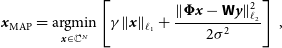 \begin{equation} \textbf{x}_{\rm MAP} = \mathop{\rm argmin}_{\textbf{x} \in \mathbb{C}^N} \left[\gamma\|\textbf{x} \|_{\ell_1} + \frac{\|{\boldsymbol{\Phi}}\textbf{x} - \textbf{W}\textbf{y} \|_{\ell_2}^2}{2\sigma^2}\right]\ ,\end{equation}
where the
 $\ell_p$
-norm is defined as
$\ell_p$
-norm is defined as
 $\|\textbf{a} \|_{\ell_p} = (\sum_k|a_k|^p)^{1/p}$
. This problem is unconstrained with
$\|\textbf{a} \|_{\ell_p} = (\sum_k|a_k|^p)^{1/p}$
. This problem is unconstrained with
 $\gamma$
as a parameter to be determined, and
$\gamma$
as a parameter to be determined, and
 $\sigma$
is the root mean-squared (RMS) uncertainty on the measurements. This is the convex optimisation problem solved by Li et al. (Reference Li, Brown, Cornwell and de Hoog2011) and Andrecut et al. (Reference Andrecut, Stil and Taylor2012). When the noise vector has uncorrelated components and an RMS uncertainty
$\sigma$
is the root mean-squared (RMS) uncertainty on the measurements. This is the convex optimisation problem solved by Li et al. (Reference Li, Brown, Cornwell and de Hoog2011) and Andrecut et al. (Reference Andrecut, Stil and Taylor2012). When the noise vector has uncorrelated components and an RMS uncertainty
 $\sigma_k$
for component
$\sigma_k$
for component
 $\textbf{n}_k$
, the weights are diagonal and should be chosen to be
$\textbf{n}_k$
, the weights are diagonal and should be chosen to be
 $\textbf{W}_{kk} = \sigma/\sigma_k$
. We then choose
$\textbf{W}_{kk} = \sigma/\sigma_k$
. We then choose
 $\sigma = \frac{1}{\sqrt{\sum_{k=1}^{M} 1/\sigma_k^2}}$
to ensure that
$\sigma = \frac{1}{\sqrt{\sum_{k=1}^{M} 1/\sigma_k^2}}$
to ensure that
 $\sum_{k = 1}^M |\textbf{W}_{kk}|^2 = M$
, and any further normalisation is in the definition of the Fourier relation and measurement equation.
$\sum_{k = 1}^M |\textbf{W}_{kk}|^2 = M$
, and any further normalisation is in the definition of the Fourier relation and measurement equation.
The CLEAN style prior can be recast as a constrained
 $\ell_1$
-regularisation problem
$\ell_1$
-regularisation problem
 \begin{equation} \textbf{x}_{\rm Const.} = \mathop{\rm argmin}_{\textbf{x} \in \mathbb{C}^N} \left[\|\textbf{x} \|_{\ell_1} + \iota_{\mathcal{B}^\varepsilon(\textbf{W}\textbf{y})}({\boldsymbol{\Phi}}\textbf{x})\right]\, , \end{equation}
where we are constraining our solution to lie close to the measurements
 $\textbf{y}$
using an indicator function defined as
$\textbf{y}$
using an indicator function defined as
 $\iota_{\mathcal{U}}(\textbf{a}) = 0$
when
$\iota_{\mathcal{U}}(\textbf{a}) = 0$
when
 $\textbf{a} \in \mathcal{U}$
and
$\textbf{a} \in \mathcal{U}$
and
 $\iota_{\mathcal{U}}(\textbf{a}) = +\infty$
otherwise. The
$\iota_{\mathcal{U}}(\textbf{a}) = +\infty$
otherwise. The
 $\ell_2$
-ball set
$\ell_2$
-ball set
 $\mathcal{B}^\varepsilon(\textbf{y})$
is defined as
$\mathcal{B}^\varepsilon(\textbf{y})$
is defined as
 $ \mathcal{B}^\varepsilon(\textbf{W}\textbf{y}) = \{ \textbf{z}:\|\textbf{z} - \textbf{W}\textbf{y} \|_{\ell_2} \leq \varepsilon \}$
and
$ \mathcal{B}^\varepsilon(\textbf{W}\textbf{y}) = \{ \textbf{z}:\|\textbf{z} - \textbf{W}\textbf{y} \|_{\ell_2} \leq \varepsilon \}$
and
 $\varepsilon$
is a tolerance related to
$\varepsilon$
is a tolerance related to
 $\sigma$
. The constrained formulation is closely related to the unconstrained problem and was previously used by Pratley & Johnston-Hollitt (Reference Pratley and Johnston-Hollitt2020). We can add more indicator functions or penalties as a prior to put further restrictions on the set of solutions.
$\sigma$
. The constrained formulation is closely related to the unconstrained problem and was previously used by Pratley & Johnston-Hollitt (Reference Pratley and Johnston-Hollitt2020). We can add more indicator functions or penalties as a prior to put further restrictions on the set of solutions.
As discussed in Section 3, since no flux can be observed for
 $\lambda^2 \leq 0$
there is no way to constrain the fit over this range. Ignoring P(0), there are special cases where the non-observable flux from
$\lambda^2 \leq 0$
there is no way to constrain the fit over this range. Ignoring P(0), there are special cases where the non-observable flux from
 $\lambda^2 \leq 0$
can be determined from observations of flux from
$\lambda^2 \leq 0$
can be determined from observations of flux from
 $\lambda^2 > 0$
. One special case is when
$\lambda^2 > 0$
. One special case is when
 $F(\phi)$
is a Hermitian function which results in the relation
$F(\phi)$
is a Hermitian function which results in the relation
 $P^*(\!-|\lambda^2|) = P(|\lambda^2|)$
. However, in general, the potential to introduce structure over the range
$P^*(\!-|\lambda^2|) = P(|\lambda^2|)$
. However, in general, the potential to introduce structure over the range
 $\lambda^2 \leq 0$
is an unavoidable problem because every fitted RM component (e.g. the basis function
$\lambda^2 \leq 0$
is an unavoidable problem because every fitted RM component (e.g. the basis function
 ${\rm e}^{2i\lambda^2\phi}$
) will parameterise the entire
${\rm e}^{2i\lambda^2\phi}$
) will parameterise the entire
 $\lambda^2$
domain. Furthermore, constraining flux to be zero for
$\lambda^2$
domain. Furthermore, constraining flux to be zero for
 $\lambda^2 \leq 0$
limits the support of
$\lambda^2 \leq 0$
limits the support of
 $P(\lambda^2)$
, this requires the fitted signal to need more RM components and would not be promoted by a sparsity prior alone.
$P(\lambda^2)$
, this requires the fitted signal to need more RM components and would not be promoted by a sparsity prior alone.
We can solve for the solution presented in Equations (8) and (9) to ensure that
 $P(\lambda^2) \to 0$
as
$P(\lambda^2) \to 0$
as
 $\lambda^2 \to 0$
and
$\lambda^2 \to 0$
and
 $P(\lambda^2) = 0$
for
$P(\lambda^2) = 0$
for
 $\lambda^2 \leq 0$
, which is discussed in Section 3, so that a solution will have a Faraday spectrum that can in-principle be constrained against future observations. To do this we suggest the modification
$\lambda^2 \leq 0$
, which is discussed in Section 3, so that a solution will have a Faraday spectrum that can in-principle be constrained against future observations. To do this we suggest the modification
 \begin{equation} \textbf{x}_{\rm Const.} = \mathop{\rm argmin}_{\textbf{x} \in \mathbb{C}^N} \left[\|\textbf{x} \|_{\ell_1} + \iota_{\mathcal{B}^\varepsilon(\textbf{W}\textbf{y})}({\boldsymbol{\Phi}}\textbf{x})+ \iota_{\mathcal{C}}(\textbf{F}\textbf{x})\right] \, , \end{equation}
where
 $\textbf{F} \in \mathbb{C}^{N\times N}$
is a Fourier transform from
$\textbf{F} \in \mathbb{C}^{N\times N}$
is a Fourier transform from
 $\phi$
-space to
$\phi$
-space to
 $\lambda^2$
-space, and
$\lambda^2$
-space, and
 $\mathcal{C} \subset \mathbb{C}^N$
is the set where
$\mathcal{C} \subset \mathbb{C}^N$
is the set where
 $\textbf{z}$
is zero for
$\textbf{z}$
is zero for
 $\lambda^2 \leq 0$
for all
$\lambda^2 \leq 0$
for all
 $\textbf{z}\in \mathcal{C}$
. While solving Equation (19), we use Equation (8) to project onto the set of solutions that satisfy
$\textbf{z}\in \mathcal{C}$
. While solving Equation (19), we use Equation (8) to project onto the set of solutions that satisfy
 $P(\lambda^2) = P_{\lambda^2 > 0}(\lambda^2)$
within the primal-dual algorithm (Combettes et al. Reference Combettes, Condat, Pesquet and Vu2014). Furthermore, we can modify the constraining
$P(\lambda^2) = P_{\lambda^2 > 0}(\lambda^2)$
within the primal-dual algorithm (Combettes et al. Reference Combettes, Condat, Pesquet and Vu2014). Furthermore, we can modify the constraining
 $\mathcal{C}$
to be resolution limited in Faraday depth, for example, solutions that have zero flux beyond the largest observed wavelength.; however, the impact of this appears negligible when tested by the authors.
$\mathcal{C}$
to be resolution limited in Faraday depth, for example, solutions that have zero flux beyond the largest observed wavelength.; however, the impact of this appears negligible when tested by the authors.
5. The simulated and observed impact of
 $\boldsymbol{\lambda}^{\textbf{2}} \boldsymbol{\leq} \textbf{0}$

We demonstrate that the prior for
 $\lambda^2 \leq 0$
can make a difference in the recovered result. One way to affect the resultant spectrum is to retain total intensity spectral structure. For a Faraday thin screen with Faraday rotation component
$\lambda^2 \leq 0$
can make a difference in the recovered result. One way to affect the resultant spectrum is to retain total intensity spectral structure. For a Faraday thin screen with Faraday rotation component
 $\phi_0$
, we can write
$\phi_0$
, we can write
 $F(\phi) = pK (\phi - \phi_0)$
; here we show that the choice of prior implicitly fits a model over
$F(\phi) = pK (\phi - \phi_0)$
; here we show that the choice of prior implicitly fits a model over
 $\lambda^2 \leq 0$
.
$\lambda^2 \leq 0$
.
As a demonstration, we simulate observations of the polarisation signals
 $P(\lambda^2) = I(\lambda^2)$
and
$P(\lambda^2) = I(\lambda^2)$
and
 $P(\lambda^2) = I(\lambda^2) {\rm e}^{2i\lambda^2 100}$
, where I is spectral structure for a synchrotron spectrum defined by Equation (5.90) of Condon & Ransom (Reference Condon and Ransom2016). We simulate
$P(\lambda^2) = I(\lambda^2) {\rm e}^{2i\lambda^2 100}$
, where I is spectral structure for a synchrotron spectrum defined by Equation (5.90) of Condon & Ransom (Reference Condon and Ransom2016). We simulate
 $M = 128$
observed frequency channels that are equally spaced between 1.3 and 9.7 GHz. We then band-limit the signal by the longest wavelength in
$M = 128$
observed frequency channels that are equally spaced between 1.3 and 9.7 GHz. We then band-limit the signal by the longest wavelength in
 $\lambda^2$
-space and use a Fourier Transform to create
$\lambda^2$
-space and use a Fourier Transform to create
 $\textbf{x}_{\rm true}$
in Faraday depth. In interferometeric imaging, the potential reconstructed resolution is higher for large signal-to-noise ratios when using a CLEAN style prior. However, because the flux of our models is not a flat spectrum the total flux can increase or decrease with more Faraday resolution, we don’t expect to accurately super-resolve the model. We follow the Nyquist resolution formula
$\textbf{x}_{\rm true}$
in Faraday depth. In interferometeric imaging, the potential reconstructed resolution is higher for large signal-to-noise ratios when using a CLEAN style prior. However, because the flux of our models is not a flat spectrum the total flux can increase or decrease with more Faraday resolution, we don’t expect to accurately super-resolve the model. We follow the Nyquist resolution formula
 $\delta \phi \leq \frac{\pi}{2\lambda^2_{\rm max}}$
; with
$\delta \phi \leq \frac{\pi}{2\lambda^2_{\rm max}}$
; with
 $\lambda^2_{\rm max} = 0.0532$
we choose the resolution which is approximately twice the Nyquist sampling rate
$\lambda^2_{\rm max} = 0.0532$
we choose the resolution which is approximately twice the Nyquist sampling rate
 $\delta \phi = 15$
rad m-2.Footnote
6
We add Gaussian noise to the Stokes Q and U linear polarisations individually where
$\delta \phi = 15$
rad m-2.Footnote
6
We add Gaussian noise to the Stokes Q and U linear polarisations individually where
 $P = Q + iU$
, following the formula for the RMS
$P = Q + iU$
, following the formula for the RMS
 \begin{equation} \sigma = \|{\boldsymbol{\Phi}}\textbf{x}_{\rm true} \|_{\ell_2}\frac{10^{-\frac{\rm ISNR}{20}}}{\sqrt{2M}}\, , \end{equation}
where ISNR is the input signal-to-noise ratio. This allows us to calculate
 $\varepsilon = \sqrt{2M + \sqrt{4M}}\sigma$
for ISNR
$\varepsilon = \sqrt{2M + \sqrt{4M}}\sigma$
for ISNR
 $= 30$
dB.
$= 30$
dB.
Figure 2 shows comparisons of the reconstructions with and without constraining
 $P_{\lambda^2 \leq 0}(\lambda^2) = 0$
. When there is sufficient spectral structure, there is a multi-peaked structure due to flux from
$P_{\lambda^2 \leq 0}(\lambda^2) = 0$
. When there is sufficient spectral structure, there is a multi-peaked structure due to flux from
 $\lambda^2 \leq 0$
in the solution even when there is no Faraday rotation in the signal. We also show that this is true for non-zero RM values. In cases where there are no multi-peaks introduced into the Faraday spectrum, there is less unconstrained flux for
$\lambda^2 \leq 0$
in the solution even when there is no Faraday rotation in the signal. We also show that this is true for non-zero RM values. In cases where there are no multi-peaks introduced into the Faraday spectrum, there is less unconstrained flux for
 $\lambda^2 \leq 0$
. We show that adding the
$\lambda^2 \leq 0$
. We show that adding the
 $P_{\lambda^2 \leq 0}(\lambda^2) = 0$
constraint can remove structure introduced in model fitting over the range
$P_{\lambda^2 \leq 0}(\lambda^2) = 0$
constraint can remove structure introduced in model fitting over the range
 $\lambda^2 \leq 0$
. This suggests that phase information from
$\lambda^2 \leq 0$
. This suggests that phase information from
 $\lambda^2 \leq 0$
is a major contribution in this case. We calculate the normalised root mean-squared error (NRMSE) between each reconstructed and ground truth Faraday spectrum using the formula
$\lambda^2 \leq 0$
is a major contribution in this case. We calculate the normalised root mean-squared error (NRMSE) between each reconstructed and ground truth Faraday spectrum using the formula
 ${\rm NRMSE} = \|\textbf{x}_{\rm true} - \textbf{x}_{\rm Const.} \|_{\ell_2}/\|\textbf{x}_{\rm true} \|_{\ell_2}$
. For the reconstructions and ground truths shown in column 3 of Figure 2, the NRMSE for rows 1–4 for
${\rm NRMSE} = \|\textbf{x}_{\rm true} - \textbf{x}_{\rm Const.} \|_{\ell_2}/\|\textbf{x}_{\rm true} \|_{\ell_2}$
. For the reconstructions and ground truths shown in column 3 of Figure 2, the NRMSE for rows 1–4 for
 $F^{\rm Model}_{\lambda^2 > 0}(\phi)$
and
$F^{\rm Model}_{\lambda^2 > 0}(\phi)$
and
 $F^{\rm Model}(\phi)$
are shown in Figure 3. The NRMSE is lower when constraining the flux to be zero for
$F^{\rm Model}(\phi)$
are shown in Figure 3. The NRMSE is lower when constraining the flux to be zero for
 $\lambda^2 \leq 0$
, and it is comparable when the breaking frequency is not observed.
$\lambda^2 \leq 0$
, and it is comparable when the breaking frequency is not observed.
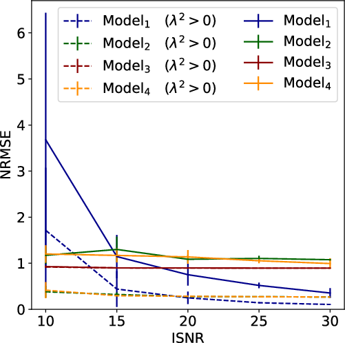
Figure 3. The NRMSE for the reconstructed Faraday spectra seen in the rows of Figure 2 (models 1–4 represent rows 1–4) for different ISNR. The error bars are centred at the mean value over 10 noise realisations and have the length given by the standard deviation.
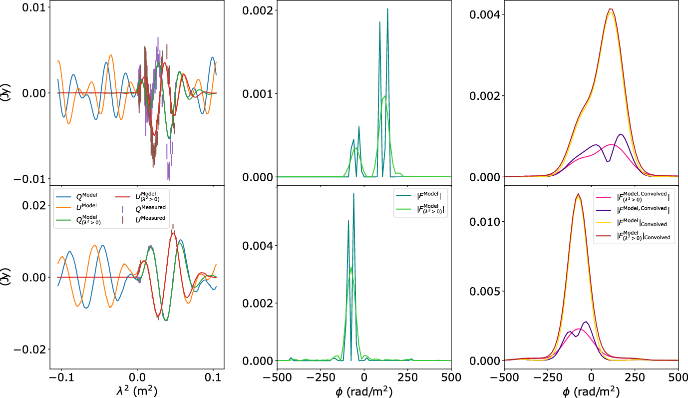
Figure 4. Reconstructions of observed spectra using a CLEAN style prior in Faraday depth with and without the prior of
 $P_{\lambda^2 \leq 0}(\lambda^2) = 0$
, for the sources lmc_c15 (top row) and cena_c1972 (bottom row) from Anderson et al. (Reference Anderson, Gaensler and Feain2016). Columns (left to right) are measurements and fitted models in
$P_{\lambda^2 \leq 0}(\lambda^2) = 0$
, for the sources lmc_c15 (top row) and cena_c1972 (bottom row) from Anderson et al. (Reference Anderson, Gaensler and Feain2016). Columns (left to right) are measurements and fitted models in
 $\lambda^2$
coordinates, the fitted Faraday spectra, and the convolved Faraday spectra (where the convolutions are applied to each of the complex and absolute valued spectra).
$\lambda^2$
coordinates, the fitted Faraday spectra, and the convolved Faraday spectra (where the convolutions are applied to each of the complex and absolute valued spectra).
The wavelength squared range shown in Figure 2 is between the values of
 $\lambda^2 = \pm \frac{\pi}{2\delta \phi}$
which is
$\lambda^2 = \pm \frac{\pi}{2\delta \phi}$
which is
 $\pm 0.104$
m
$\pm 0.104$
m
 $^2$
when the Fast Fourier Transform (FFT) grid has a resolution of
$^2$
when the Fast Fourier Transform (FFT) grid has a resolution of
 $\delta \phi = 15$
rad m−2. This is the spacing of the periodic boundary conditions imposed by the Fourier series calculated using the FFT. It is important to show the full periodic range for two reasons. The first reason is that this transform can be inverted using an FFT, which means that no information is lost between the two signals. The second reason is that it is important to see that the signal wraps around at the boundaries, this phenomena is also known as aliasing. Figure 2 shows that
$\delta \phi = 15$
rad m−2. This is the spacing of the periodic boundary conditions imposed by the Fourier series calculated using the FFT. It is important to show the full periodic range for two reasons. The first reason is that this transform can be inverted using an FFT, which means that no information is lost between the two signals. The second reason is that it is important to see that the signal wraps around at the boundaries, this phenomena is also known as aliasing. Figure 2 shows that
 $P_{\lambda^2 \geq 0}(\lambda^2)$
tends towards zero for large
$P_{\lambda^2 \geq 0}(\lambda^2)$
tends towards zero for large
 $\lambda^2$
for this reason, for example, the structure of flux at large negative
$\lambda^2$
for this reason, for example, the structure of flux at large negative
 $\lambda^2$
will impact the structure of flux at large positive
$\lambda^2$
will impact the structure of flux at large positive
 $\lambda^2$
. The largest
$\lambda^2$
. The largest
 $\lambda^2$
coordinate in the model and the ground truth is (
$\lambda^2$
coordinate in the model and the ground truth is (
 $0.104$
m
$0.104$
m
 $^2$
) is twice the largest coordinate in the observed signal (
$^2$
) is twice the largest coordinate in the observed signal (
 $0.0532$
m
$0.0532$
m
 $^2$
), both of the fitted models show deviations from the ground truth spectra above
$^2$
), both of the fitted models show deviations from the ground truth spectra above
 $0.0532$
m
$0.0532$
m
 $^2$
.
$^2$
.
Figure 4 demonstrates the effect and solution for two real observations from Anderson et al. (Reference Anderson, Gaensler and Feain2016). The sources lmc_c15 and cena_c1972 were observed between 1 and 10 GHz using the Australia Telescope Compact Array. The results from Anderson et al. (Reference Anderson, Gaensler and Feain2016) show that the single component QU fit seen for cena_c1972 is consistent with the peak after the
 $\lambda^2 \leq 0$
correction; the three component QU fit for lmc_c15 is consistent to fitting two peaks to one component and a single peak to the other component after the
$\lambda^2 \leq 0$
correction; the three component QU fit for lmc_c15 is consistent to fitting two peaks to one component and a single peak to the other component after the
 $\lambda^2 \leq 0$
correction. Using non-parametric QU-fitting we find a smooth curve with one peak per component (lmc_c15: 114
$\lambda^2 \leq 0$
correction. Using non-parametric QU-fitting we find a smooth curve with one peak per component (lmc_c15: 114
 $\pm$
24.5 and
$\pm$
24.5 and
 $-50.8$
 $\pm$
25.0 rad m-2; cena_c1972:
$\pm$
25.0 rad m-2; cena_c1972:
 $-75.3$
 $\pm$
28.1 rad m-2), while fitting the spectral structure. These Faraday RM results provided in Figure 4 are calculated by absolute flux weighting for the mean and standard deviation of Faraday depth coordinates
$\pm$
28.1 rad m-2), while fitting the spectral structure. These Faraday RM results provided in Figure 4 are calculated by absolute flux weighting for the mean and standard deviation of Faraday depth coordinates
 $\phi$
with polarised flux above
$\phi$
with polarised flux above
 $0.1 \times F(\phi_{\rm peak})$
. Specifically, we define the region of integration for a single component as
$0.1 \times F(\phi_{\rm peak})$
. Specifically, we define the region of integration for a single component as
 $S = \{\phi: 0.1 \times |F(\phi_{\rm peak})| < |F(\phi)| \}$
and calculate the flux weighted mean
$S = \{\phi: 0.1 \times |F(\phi_{\rm peak})| < |F(\phi)| \}$
and calculate the flux weighted mean
 $\langle {\rm RM} \rangle$
and standard deviation
$\langle {\rm RM} \rangle$
and standard deviation
 $\sigma_{{\rm RM}}$
as
$\sigma_{{\rm RM}}$
as
 \begin{equation} \langle {\rm RM} \rangle = \frac{\sum_{\phi \in S} |F(\phi)| \phi }{\sum_{\phi \in S} |F(\phi)| }\, ,\end{equation}
and
 \begin{equation} \sigma_{{\rm RM}}^2 = \frac{\sum_{\phi \in S} |F(\phi)| (\phi - \langle {\rm RM} \rangle)^2}{\sum_{\phi \in S} |F(\phi)| } \, . \end{equation}
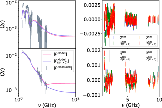
Figure 5. The magnitude and residuals for the fitted signals from Figure 4 are shown for observations of sources lmc_c15 (top row) and cena_c1972 (bottom row). The magnitude of the fitted linear polarisation intensities and corresponding observations in
 $\nu$
coordinates as a logarithmic scale in the left column. The residuals for the fitted signals
$\nu$
coordinates as a logarithmic scale in the left column. The residuals for the fitted signals
 $Q^{\rm Res} = Q^{\rm Measured} - Q^{\rm Model}$
and
$Q^{\rm Res} = Q^{\rm Measured} - Q^{\rm Model}$
and
 $U^{\rm Res} = U^{\rm Measured} - U^{\rm Model}$
in linear scale in right column. We find that constraining
$U^{\rm Res} = U^{\rm Measured} - U^{\rm Model}$
in linear scale in right column. We find that constraining
 $P_{\lambda^2 \leq 0}(\lambda^2) = 0$
provides a similar magnitude for the residuals, this follows because they are solutions to Equations (18) and (19).
$P_{\lambda^2 \leq 0}(\lambda^2) = 0$
provides a similar magnitude for the residuals, this follows because they are solutions to Equations (18) and (19).
Figure 4 shows that the signals with and without non-observable structure provide similar fits to the observed spectra for
 $\lambda^2 > 0$
in the presence of curvature. However, the structure for
$\lambda^2 > 0$
in the presence of curvature. However, the structure for
 $\lambda^2 \leq 0$
is not constrained by the observation and imposes multiple peaks in the reconstructed signal. Figure 5 shows that both constraining and unconstraining the
$\lambda^2 \leq 0$
is not constrained by the observation and imposes multiple peaks in the reconstructed signal. Figure 5 shows that both constraining and unconstraining the
 $\lambda^2 \leq 0$
interval to zero does not greatly change the residuals in each fit, which is expected from the fidelity constraint.
$\lambda^2 \leq 0$
interval to zero does not greatly change the residuals in each fit, which is expected from the fidelity constraint.
In many contexts, double peaked structures can be removed by resolution limiting the signal, but this does not remove the double peaked structures for these examples. Resolution limiting the polarisation magnitude
 $|F(\phi)|$
will remove these structures, this suggests that the phase is partially responsible for the double peaks (a similar phase issue has been discussed in Farnsworth et al. Reference Farnsworth, Rudnick and Brown2011). However, smoothing the magnitude is a non-linear process and we do not suggest it as a method.
$|F(\phi)|$
will remove these structures, this suggests that the phase is partially responsible for the double peaks (a similar phase issue has been discussed in Farnsworth et al. Reference Farnsworth, Rudnick and Brown2011). However, smoothing the magnitude is a non-linear process and we do not suggest it as a method.
The reconstructions were performed using a MacBook Pro (2019) with 4 cores (2.4 GHz) and 16 GB of RAM. 50 000 iterations took approximately 15 seconds which we consider an upper bound on reconstruction time for each line of sight. However, convergence can typically be reached in 100–1 000 s of iterations which takes approximately a second or less. Each iteration applies
 ${\boldsymbol{\Phi}}$
and
${\boldsymbol{\Phi}}$
and
 ${\boldsymbol{\Phi}}^\dagger$
which can be applied as either a direct matrix multiplication or using a Non-Uniform Fast Fourier transform (NUFFT). To enforce the constraint on flux in
${\boldsymbol{\Phi}}^\dagger$
which can be applied as either a direct matrix multiplication or using a Non-Uniform Fast Fourier transform (NUFFT). To enforce the constraint on flux in
 $\lambda^2$
space we need to perform an FFT and its inverse for each iteration. We can use the 15 s upper bound and estimate 4 200 h of serial computation to reconstruct 1 000 000 independent lines of sight (e.g. which we could expect in a full POSSUM catalogue; Gaensler et al. Reference Gaensler, Landecker and Taylor2010). Using a single high performance workstation with 64 cores in parallel this can be reduced to approximately an hour of computation. We provide a public Python implementation of the algorithm used in this work at https://github.com/Luke-Pratley/Faraday-Dreams.
$\lambda^2$
space we need to perform an FFT and its inverse for each iteration. We can use the 15 s upper bound and estimate 4 200 h of serial computation to reconstruct 1 000 000 independent lines of sight (e.g. which we could expect in a full POSSUM catalogue; Gaensler et al. Reference Gaensler, Landecker and Taylor2010). Using a single high performance workstation with 64 cores in parallel this can be reduced to approximately an hour of computation. We provide a public Python implementation of the algorithm used in this work at https://github.com/Luke-Pratley/Faraday-Dreams.
We have shown that structures caused by fitted flux over
 $\lambda^2 \leq 0$
provides us with a smooth spectrum with a single peak for each Faraday screen. Without this constraint, we would arrive at a different scientific conclusion on the number of Faraday components. We have also found consistent results for the other observed broadband sources of Anderson et al. (Reference Anderson, Gaensler and Feain2016).
$\lambda^2 \leq 0$
provides us with a smooth spectrum with a single peak for each Faraday screen. Without this constraint, we would arrive at a different scientific conclusion on the number of Faraday components. We have also found consistent results for the other observed broadband sources of Anderson et al. (Reference Anderson, Gaensler and Feain2016).
6. Conclusions
We have shown that non-observable structures can be introduced into fitted models of Faraday rotation spectra when the flux for
 $\lambda^2 \leq 0$
is not constrained. We show that by setting the prior flux to zero over this range, we can remove the structures introduced from the unconstrained
$\lambda^2 \leq 0$
is not constrained. We show that by setting the prior flux to zero over this range, we can remove the structures introduced from the unconstrained
 $\lambda^2 \leq 0$
region. We demonstrate the effect of this constraint using non-parametric QU-fitting on both simulations and real data. Without an explicit prior or constraint on
$\lambda^2 \leq 0$
region. We demonstrate the effect of this constraint using non-parametric QU-fitting on both simulations and real data. Without an explicit prior or constraint on
 $\lambda^2 \leq 0$
there can always be some contribution to the reconstructed Faraday rotation signal that is not possible to compare against future observations. This constraint will be needed when interpreting Faraday structures from next-generation broadband radio telescopes where it can impact the scientific conclusion. Current RMCLEAN algorithms do not have the ability to restrict the recovered flux only for
$\lambda^2 \leq 0$
there can always be some contribution to the reconstructed Faraday rotation signal that is not possible to compare against future observations. This constraint will be needed when interpreting Faraday structures from next-generation broadband radio telescopes where it can impact the scientific conclusion. Current RMCLEAN algorithms do not have the ability to restrict the recovered flux only for
 $\lambda^2 > 0$
. This will be needed in the context of interferometric observations of extended sources where fractional polarisation can be non-physical, for example, the interstellar medium (Gaensler et al. Reference Gaensler2011). This work shows how developments in convex optimisation and polarimetric theory over the last 10 yr can be leveraged for improved Faraday depth fidelity in broadband observations.
$\lambda^2 > 0$
. This will be needed in the context of interferometric observations of extended sources where fractional polarisation can be non-physical, for example, the interstellar medium (Gaensler et al. Reference Gaensler2011). This work shows how developments in convex optimisation and polarimetric theory over the last 10 yr can be leveraged for improved Faraday depth fidelity in broadband observations.
Acknowledgements
The Dunlap Institute is funded through an endowment established by the David Dunlap family and the University of Toronto. MJ-H thanks T. Olsson, Ø. Berøy, & A. Sørlie for motivation in the Long Night over which this manuscript was edited. BMG acknowledges the support of the Natural Sciences and Engineering Research Council of Canada (NSERC) through grant RGPIN-2015-05948, and of the Canada Research Chairs programme. We thank the referee for their careful reading and constructive comments.