


1. Introduction
Transformer (Vaswani et al. Reference Vaswani, Shazeer, Parmar, Uszkoreit, Jones, Gomez, Kaiser and Polosukhin2017), a fully connected self-attention architecture, is a core module of recent neural network language models. By utilizing the idea of convolutional neural network (CNN) (LeCun et al. Reference LeCun and Bengio1995) and self-attention, Transformers significantly reduced the time complexity during model training and gained improved parallel performance. However, the self-attention mechanism is insensitive to the order of the input sequence (i.e., it is an operation on sets, Pham et al. Reference Pham, Bui, Mai and Nguyen2020). That is, for input sequences with same constituent words but different orders, Transformers produce same predictions. Word order is one of the basic grammatical devices of natural language and an important method of meaning representation. To endow the model with word order awareness, Transformers are reinforced with position information by means of position encoding/embedding (PE) to discriminate input sequences of different orders.
To date, although a variety of methods for incorporating position information into Transformers have been proposed (see Wang and Chen Reference Wang and Chen2020; Dufter, Schmitt, and Schütze Reference Dufter, Schmitt and Schütze2021 for a review), most of these methods are proposed based on researchers’ intuition. It is, therefore, reasonable to ask: how can position information be encoded in a principled way?
Developing a workable method of PE for Transformers is a tricky attempt with superficial simplicity. In our following analysis, we first try to understand what it means for models to have the position information of words. After that, we explore what kind of position-related information should be factored into the architecture of the Transformer.
The practical success of recent neural network language models can simply be attributed to the utilization of co-occurrence relations between words. The purpose of incorporating position information is to enable models to discriminate sentences with same constituent words but different permutations of words (failing to do so results in bag-of-words models). For a specific model, word sequences of different permutations should be assigned different probabilities. If the permutation of words does not affect the frequency of a word sequence, then the input of position information is meaningless.
Then, what kind of position-related factors do affect the frequency of word sequences? Absolute position? Relative position? Or some other factors? Theoretically speaking, all position-related factors should be considered in the further improvement of Transformers’ PE architectures.
To answer this question, we provide a detailed analysis of the position of language units. An “axiom” of all neural network language models is the idea of the distributional hypothesis: “words which are similar in meaning occur in similar contexts” (Harris Reference Harris1954). Therefore, to discriminate word sequences of different permutations is, in essence, to identify the context in which a focus word occurs. Or, in other words, to model the context.
Context is a complicated concept with broad senses (Hess, Foss, and Carroll Reference Hess, Foss and Carroll1995; Otten and Van Berkum Reference Otten and Van Berkum2008), involving both syntax and semantics. Context has its influence locally within a sentence and globally between words separated by long distances (Schenkel, Zhang, and Zhang Reference Schenkel, Zhang and Zhang1993; Ebeling and Pöschel Reference Ebeling and Pöschel1994; Alvarez-Lacalle et al. Reference Alvarez-Lacalle, Dorow, Eckmann and Moses2006; Altmann, Cristadoro, and Degli Esposti Reference Altmann, Cristadoro and Degli Esposti2012). Meanwhile, context is affected by either preceding or following language units. Even messages that are not linguistically encoded have their influence on a context. As a result, to model the context quantitatively or include all contextual information in a single model is a challenging task. In this regard, richer and more comprehensive context information is thus essential to the further improvement of language models. Therefore, it is arguable that the development of language models can be seen, to some extent, as the development of context models.
A feasible but oversimplified approach to model the context of a focus word is to identify words before and after it. Among the most popular models following this fashion are statistical models like N-gram (Jelinek Reference Jelinek1997; Rosenfeld Reference Rosenfeld2000; Zhai Reference Zhai2008), latent semantic analysis (LSA) (Deerwester et al. Reference Deerwester, Dumais, Furnas, Landauer and Harshman1990), and static neural network word embeddings like Word2Vec (Mikolov et al. Reference Mikolov, Chen, Corrado and Dean2013) and GloVe (Pennington, Socher, and Manning Reference Pennington, Socher and Manning2014). However, these models have their limitations. For example, N-gram models take into consideration only
 $n-1$
words before the word to be predicted; models like Word2Vec and GloVe are bag-of-words models. With the advent of self-attention mechanism in neural network language models, the context window has been expanded to full sentence and even beyond. Compared with the previous context models, the self-attention mechanism models context implicitly as it does not discriminate words in different positions. Transformers thus need word position information as input.
$n-1$
words before the word to be predicted; models like Word2Vec and GloVe are bag-of-words models. With the advent of self-attention mechanism in neural network language models, the context window has been expanded to full sentence and even beyond. Compared with the previous context models, the self-attention mechanism models context implicitly as it does not discriminate words in different positions. Transformers thus need word position information as input.
We consider position information to be an essential ingredient of context. A neural network language model reinforced with position-related information can predict the probability of words, sentences, and even texts more accurately and thus better represent the meaning of linguistic units. Therefore, we believe that all position-related information that affects the output probability should be considered in the modeling of PE.
To incorporate more position-related information, some studies provide language models with syntactic structures (such as dependency trees, Wang et al. Reference Wang, Wang, Chen, Wang and Kuo2019a), only to deliver marginal improvements in downstream tasks. Therefore, a detailed analysis of factors that affect the probability of word sequences is needed.
In this study, we first examined the position-related factors that affect the frequency of words, such as absolute position and sentence length. This effort provides guidance to the development of absolute position encoding/embedding (APE) schemas. We then focused on factors that influence the frequency of bigrams, which will guide the development of relative position encoding/embedding (RPE) schemas. Finally, with the study of the co-occurrence frequency of the nominative and genitive forms of English personal pronouns, we observed that the frequency distribution of these bigrams over relative position carry meaningful linguistic knowledge, which suggests that a more complex input method of position information may bring us extra grammatical information.
Although our research focus merely on the position distribution of unigrams and bigrams, the conclusion we made can provide a basis for studying the relationships between multiple words, since more intricate relationships among more words can be factored into multiple two-word relationships. For example, dependency parsing treats the multi-word relationships in a sentence (as a multi-word sequence) as a set of two-word relationships: each sentence is parsed into a set of dependency relations and each dependency relationship is a two-word relation between a dependent word and its head word (Liu Reference Liu2008, Reference Liu2010).
2. Position encoding/embedding
Methods for incorporating position information introduced in previous researches can be subsumed under two categories: plain-text-based methods and structured-text-based methods. The former does not require any processing of input texts, while the latter analyzes the structures of input texts.
Before further analysis, we distinguish between two concepts: position encoding and position embedding. Strictly speaking, position encoding refers to fixed position representation (such as sinusoidal position encoding), while position embedding refers to learned position representation. Although these two concepts are used interchangeably in many studies, we make a strict distinction between the two in this study.
2.1. Plain-text-based position encoding/embedding
In previous researches, Transformer-based language models are fed with absolute and relative position of words. These two types of information are further integrated into models in two ways: fixed encoding and learned embedding. APE focuses on the linear position of a word in a sentence, while RPE deals with the difference between the linear position of two words in a sentence. Current studies have not observed significant performance differences between the two PE schemas (Vaswani et al. Reference Vaswani, Shazeer, Parmar, Uszkoreit, Jones, Gomez, Kaiser and Polosukhin2017). However, we believe that the linguistic meaning of the two is different. Absolute position schema specifies the order of words in a sentence. It is a less robust schema as the linear positions are subject to noise: the insertion of even a single word with little semantic impact to a sentence will alter the positions of neighboring words. Neural network language models fed with absolute positions are expected to derive the relative positions between words on its own. Relative position schema, on the other hand, specifies word–word relationships. It can be used to model the positional relationships within chunks, which are considered the building blocks of sentences. Conceivably, the relative positions between words that make up chunks are thus stable. There are also differences in how the models implement absolute and relative position schemas. By APE, WE (word embedding) and PE are summed dimension-wise to produce the final embedding of the input layer, while by RPE, position information is added to attention matrices (V and K) independent of word embeddings, which is formalized as (Wang et al. Reference Wang, Shang, Lioma, Jiang, Yang, Liu and Simonsen2021):
 \begin{equation} \mathrm{APE}\,:\left [\begin{array}{c} Q_{x} \\ K_{x} \\ V_{x} \end{array}\right ]=\left (\mathrm{WE}_{x}+P_{x}\right ) \odot \left [\begin{array}{l} W^{Q} \\ W^{K} \\ W^{V} \end{array}\right ] \quad ; \quad \mathrm{RPE}\,:\left [\begin{array}{c} Q_{x} \\ K_{x} \\ V_{x} \end{array}\right ]=\mathrm{WE}_{x} \odot \left [\begin{array}{l} W^{Q} \\ W^{K} \\ W^{V} \end{array}\right ]+\left [\begin{array}{c} \mathbf{0} \\ P_{x-y} \\ P_{x-y} \end{array}\right ] \end{equation}
The fixed position encoding encodes position information with a fixed function, while the learned position embeddings are obtained as the product of model training.
In what follows, we offer a brief introduction to the four above-mentioned PE methods.
2.1.1. Absolute position encoding
APEs (Vaswani et al. Reference Vaswani, Shazeer, Parmar, Uszkoreit, Jones, Gomez, Kaiser and Polosukhin2017) are determined in the input layer then summed with word embeddings. With this schema, absolute positions are encoded with sinusoidal functions:
 \begin{align}PE_{(pos,2i)}&=\sin\!{\left(pos/10,000^{2i/d_{\text{model}}}\right)}\nonumber\\[4pt]PE_{(\text{pos,2i+1) }}&=\cos\!{\left(pos/10,000^{2i/d_{\text{model}}}\right)}\end{align}
where
 $pos$
refer to the absolute position of a word and
$pos$
refer to the absolute position of a word and
 $d_{model}$
is the dimension of input features,
$d_{model}$
is the dimension of input features,
 $i\in [0,d/2]$
.
$i\in [0,d/2]$
.
Yan et al. (Reference Yan, Deng, Li and Qiu2019) showed that the inner product of two sinusoidal position encodings obtained by this schema is only related to the relative position between these two positions. That is, this schema enables the model to derive relative positions between words from sinusoidal position encoding. In other words, with the position encodings by this method, models have the potential to perceive the distances between words. In addition, the inner product of two position encodings decreases with the increasing relative position between two words. This suggests that the correlation between words weakens as the relative position increases. However, they also pointed out that these two seemingly good properties can be broken in actual computation. Meanwhile, the conditional probability
 $p_t|p_{t-r}=p_t|p_{t+r}$
of this encoding schema is nondirectional, which can be a disadvantage in many NLP tasks such as NER.
$p_t|p_{t-r}=p_t|p_{t+r}$
of this encoding schema is nondirectional, which can be a disadvantage in many NLP tasks such as NER.
2.1.2. Relative position encoding
Motivated by the position encoding by Vaswani et al. (Reference Vaswani, Shazeer, Parmar, Uszkoreit, Jones, Gomez, Kaiser and Polosukhin2017), Wei et al. (Reference Wei, Ren, Li, Huang, Liao, Wang, Lin, Jiang, Chen and Liu2019) proposed their RPE method as:
 \begin{align}a_{ij}\lbrack2k\rbrack & =\sin\!{\left((j-i)/{\left(10,000^\frac{2.k}{dz}\right)}\right)}\nonumber\\[3pt]a_{ij}\lbrack2k+1\rbrack & =\cos\!{\left((j-i)/{\left(10,000^\frac{2.k}{dz}\right)}\right)}\end{align}
where
 $i$
and
$i$
and
 $j$
refer to the linear position of two words in a sentence, and the definitions of
$j$
refer to the linear position of two words in a sentence, and the definitions of
 $d_z$
and
$d_z$
and
 $k$
are the same as the definitions of
$k$
are the same as the definitions of
 $d_{model}$
and
$d_{model}$
and
 $i$
in Equation (2).
$i$
in Equation (2).
A same sinusoidal RPE method is used by Yan et al. (Reference Yan, Deng, Li and Qiu2019):
 \begin{equation}R_{t-j}={\left\lbrack\dots\sin{\!\left(\frac{t-j}{10,000^{2i/d_k}}\right)}\cos{\!\left(\frac{t-j}{10,000^{2i/d_k}}\right)}\dots\right\rbrack}^T\end{equation}
with extended attention algorithm which lends direction and distance awareness to the Transformer. The sinusoidal RPE gains its advantage over sinusoidal APE not only with its direction awareness but also with its generalizability which allows the model to process longer sequences unseen in training data.
2.1.3. Absolute position embedding
Fully learnable absolute position embeddings (APEs) are first proposed by Gehring et al. (Reference Gehring, Auli, Grangier, Yarats and Dauphin2017) to model word positions in convolutional Seq2Seq architectures. By this method, the input element representations are calculated with:
 \begin{equation} e=\left(w_1+p_1,\dots,w_m+p_m\right) \end{equation}
where
 $p_m$
is a position embedding of the same size as word embedding
$p_m$
is a position embedding of the same size as word embedding
 $w_m$
at position
$w_m$
at position
 $m$
. The position embeddings and word embeddings are of same dimension but learned independently.
$m$
. The position embeddings and word embeddings are of same dimension but learned independently.
 $p_m$
is not subject to additional restrictions from
$p_m$
is not subject to additional restrictions from
 $w_m$
other than dimensionality. Both embeddings are initialized independently by sampling from a zero-mean Gaussian distribution whose standard deviation is 0.1.
$w_m$
other than dimensionality. Both embeddings are initialized independently by sampling from a zero-mean Gaussian distribution whose standard deviation is 0.1.
2.1.4. Relative position embedding
Shaw, Uszkoreit, and Vaswani (Reference Shaw, Uszkoreit and Vaswani2018) proposed a relative position embedding schema which models the input text as a labeled, directed, and fully connected graph. The relative positions between words are modeled as learnable matrices, and the schema is of direction awareness. The relative position between position
 $i$
and
$i$
and
 $j$
is defined as:
$j$
is defined as:
 \begin{equation} \begin{aligned} a_{i j}^{K} &=w_{\operatorname{clip}\!(j-i, k)}^{K} \\ a_{i j}^{V} &=w_{\operatorname{clip}(j-i, k)}^{V} \\ \operatorname{clip}\!(x, k) &=\max\! ({-}k, \min\! (k, x)) \end{aligned} \end{equation}
where
 $k$
is the maximum relative position, and
$k$
is the maximum relative position, and
 $w^K$
and
$w^K$
and
 $w^V$
are the learned relative position representations.
$w^V$
are the learned relative position representations.
2.2. Structured-text-based position encoding/embedding
The purpose of feeding a model position information is to enable it to make better use of the context. The sentence structure undoubtedly contains more contextual information and is more direct and accurate than simple position at distinguishing word meaning.
Wang et al. (Reference Wang, Tu, Wang and Shi2019b) proposed a structural position representations (SPRs) method which encodes the absolute distance between words in dependency trees with sinusoidal APE and learned RPE; Shiv and Quirk (Reference Shiv and Quirk2019) proposed an alternative absolute tree position encoding (TPE) which differs from that of Wang et al. (Reference Wang, Tu, Wang and Shi2019b) as it encodes the paths of trees rather than distances; Zhu et al. (Reference Zhu, Li, Zhu, Qian, Zhang and Zhou2019) proposed a novel structure-aware self-attention approach by which relative positions between nodes in abstract meaning representation (AMR) graphs are inputted to the model to better model the relationships between indirectly connected concepts; Schmitt et al. (Reference Schmitt, Ribeiro, Dufter, Gurevych and Schütze2020) showed their definition of RPEs in a graph based on the lengths of shortest paths. Although above methods input structurally analyzed texts to models thus offer richer positional information, the results achieved are not satisfactory.
3. Materials and methods
How should the properties of PE be studied? We argue that the purpose of incorporating PE is to enable a model to identify the word–word correlation change brought about by the change in relative position between words. And there is a close relationship between the word–word correlation and the co-occurrence probability of words.
Since the Transformer’s self-attention matrix (each row or column corresponds to a distinct word) represents the correlations between any two words in a sentence, in this paper, we investigate the correlations between words by examining the frequency distributions of word sequences consisting of two words. According to Vaswani et al. (Reference Vaswani, Shazeer, Parmar, Uszkoreit, Jones, Gomez, Kaiser and Polosukhin2017), a self-attention matrix is calculated as:
 \begin{equation} \operatorname{Attention}(Q, K, V)=\operatorname{softmax}\!\left (\frac{Q K^{T}}{\sqrt{d_{k}}}\right ) V, K=W^kI,Q=W^qI,V=W^vI \end{equation}
where
 $Q$
is the query matrix, and
$Q$
is the query matrix, and
 $K$
and
$K$
and
 $V$
are the key and value matrices, respectively.
$V$
are the key and value matrices, respectively.
 $d$
is the dimension of the input token embedding, and
$d$
is the dimension of the input token embedding, and
 $I$
is the input matrix.
$I$
is the input matrix.
In the calculation of attention, a query vector
 $q$
(as a component vector of matrix
$q$
(as a component vector of matrix
 $Q$
) obtained by transforming the embedding of an input word
$Q$
) obtained by transforming the embedding of an input word
 $w_i$
is multiplied by
$w_i$
is multiplied by
 $k$
s of all words in the sentence, regardless of whether the
$k$
s of all words in the sentence, regardless of whether the
 $k$
comes before or after it. Therefore, the correlation between
$k$
comes before or after it. Therefore, the correlation between
 $w_i$
and other words is bidirectional. In other words, with attention mechanism, the context of
$w_i$
and other words is bidirectional. In other words, with attention mechanism, the context of
 $w_i$
is modeled from both directions. Therefore, we need to model this bidirectional correlation in our research.
$w_i$
is modeled from both directions. Therefore, we need to model this bidirectional correlation in our research.
3.1. Representation of inter-word correlation
Based on the analysis in the previous section, we use k-skip-n-gram model to examine the co-occurrence probability of words. In the field of computational linguistics, a traditional k-skip-n-gram is a set of subsequences of length
 $n$
in a text, where tokens in the word sequence are separated by up to
$n$
in a text, where tokens in the word sequence are separated by up to
 $k$
tokens (Guthrie et al. Reference Guthrie, Allison, Liu, Guthrie and Wilks2006). It is a generalization of the n-gram model as the continuity of a word sequence is broken. Formally, for word sequence
$k$
tokens (Guthrie et al. Reference Guthrie, Allison, Liu, Guthrie and Wilks2006). It is a generalization of the n-gram model as the continuity of a word sequence is broken. Formally, for word sequence
 $w_1w_2\cdots w_m$
, a k-skip-n-gram is defined as:
$w_1w_2\cdots w_m$
, a k-skip-n-gram is defined as:
 \begin{equation} \text{ k-skip-n-gram }:\!=\left \{w_{i_{1}}, w_{i_{2}}, \cdots, w_{i_{n}}, \sum _{j=1}^{n} i_{j}-i_{j-1}\lt k\right \} \end{equation}
For example, in sentence “context is a complicated concept with broad senses,” the set of 3-skip-bigram starting at “context” includes: “context is,” “context a,” “context complicated,”
 $\ldots$
, “context concept.” Compared with n-gram, the k-skip-n-gram model can capture more complicated relationships between words, such as grammatical patterns and world knowledge. For instance, in the above example, “context is a concept,” a 1-skip-4-gram, clearly captures a piece of world knowledge.
$\ldots$
, “context concept.” Compared with n-gram, the k-skip-n-gram model can capture more complicated relationships between words, such as grammatical patterns and world knowledge. For instance, in the above example, “context is a concept,” a 1-skip-4-gram, clearly captures a piece of world knowledge.
For the sake of clarity and conciseness, in what follows, we give definitions of several terms used in this study.
We use the combinations of the two words that make up the k-skip-bigram and their relative positions in the original text to denote the subsequences they form. For example, in sentence “Jerry always bores Tom,” we use “Jerry Tom (3)” to denote a subsequence containing “Jerry” and “Tom” along with their relative position 3. Similarly, in sentence “Tom and Jerry is inarguably one of the most celebrated cartoons of all time,” we use “Jerry Tom (–2)” to denote a subsequence containing “Jerry” and “Tom" along with their relative position –2.
All k-skip-bigrams with the same two constituent words but different skip-distance (
 $k$
) are collectively referred to in this work as a string composed of these two words. That is, the string refers to a collection of k-skip-bigram instances. So, with the example in the previous paragraph, we use “Jerry Tom” to refer to a collection of two bigrams, that is “Jerry Tom”= {“Jerry Tom (3)”, “Jerry Tom (–2)”}. Further, we abbreviate the term “k-skip-bigram” as “bigram” to refer to k-skip-bigrams with all skips.
$k$
) are collectively referred to in this work as a string composed of these two words. That is, the string refers to a collection of k-skip-bigram instances. So, with the example in the previous paragraph, we use “Jerry Tom” to refer to a collection of two bigrams, that is “Jerry Tom”= {“Jerry Tom (3)”, “Jerry Tom (–2)”}. Further, we abbreviate the term “k-skip-bigram” as “bigram” to refer to k-skip-bigrams with all skips.
3.2. In-sentence positions and sub-corpora of equal sentence lengths
Modeling the position of language units (words and k-skip-n-grams) properly in sentences is an essential step for our study: First, it is a prerequisite for the investigation of frequency–position relationship of language units; second, since grammatical relationships can be perceived as connections between words, knowing the positions of words is therefore important for the understanding of their grammatical relationships (exemplary studies on this topic concerning dependency direction and distance can be seen in Liu Reference Liu2008 and Reference Liu2010). Despite this importance, modeling of position is often overlooked given its superficial simplicity.
Studies in psychology show that the probability of words occurring at two ends of sentences is significantly different from the probability of words appearing in the middle positions of sentences (i.e., the serial-position effect, as detailed in Hasher Reference Hasher1973; Ebbinghaus Reference Ebbinghaus2013). Therefore, our model of position should consider not only the absolute position of language units but also whether they occur at two ends of sentences. Apart from that, chunks as word sequences in sentences are of great linguistic significance. A chunk refers to words that always occur together with fixed structural relationships such as collocations and specific grammatical structure (e.g., “if
 $\ldots$
then
$\ldots$
then
 $\ldots$
”). Chunks play an important role in humans’ understanding of natural language as people infer the meanings of sentences based on known chunks. The position of a chunk in a sentence is relatively free, but the relative positions between words within it are fixed. Therefore, our model of position factors in the relative positions between words to better capture the grammatical information carried by chunks.
$\ldots$
”). Chunks play an important role in humans’ understanding of natural language as people infer the meanings of sentences based on known chunks. The position of a chunk in a sentence is relatively free, but the relative positions between words within it are fixed. Therefore, our model of position factors in the relative positions between words to better capture the grammatical information carried by chunks.
Based on the above analysis, we see that to study the relationship between the position and the frequency of language units, a model of position should consider following factors: (1) the absolute position of language units; (2) the relative position between words; and (3) whether a language unit occurs at one of the two ends of a sentence. We use natural numbers to mark the absolute position of words and integers (both positive and negative) to mark the relative positions between words. Words at the beginning of sentences can be marked with natural numbers. For example, we use 1, 2, 3 to mark the first, second, and third positions in the beginning of a sentence. However, we cannot use definite natural numbers to mark the position of words or bigrams at the end of sentences of different lengths. And, in sentences of different lengths, even if words or bigrams have the same absolute position, their positions relative to the sentences are different. For example, in a sentence of length 5, the third position is at the middle of the sentence, while in a sentence of length 10, the third position is at the beginning of the sentence. Therefore, the absolute positions of language units should not be perceived equally.
We follow the procedure below to address this problem: first, sentences in the original corpus
 $U$
(which consists of sentences of varying lengths) are divided into sub-corpora according to sentence length, which is formulated as:
$U$
(which consists of sentences of varying lengths) are divided into sub-corpora according to sentence length, which is formulated as:
 \begin{equation} U=\bigcup _{l=1}^{L}U_l,\ \forall \ s\ \in \ U_l,\ \left |s\right |=l \end{equation}
where
 $U_l$
stands for the sub-corpus of sentence length
$U_l$
stands for the sub-corpus of sentence length
 $l$
,
$l$
,
 $|s|$
is the length of sentence
$|s|$
is the length of sentence
 $s$
, and
$s$
, and
 $L$
is the number of sub-corpora, that is, the length of the longest sentences in the original corpus. Following this procedure, in each sub-corpus, when investigating the relationship between the frequency and the position of language units, the absolute positions marked with same natural number can be perceived equally, and the ending positions of sentences can be marked with integers of same meanings.
$L$
is the number of sub-corpora, that is, the length of the longest sentences in the original corpus. Following this procedure, in each sub-corpus, when investigating the relationship between the frequency and the position of language units, the absolute positions marked with same natural number can be perceived equally, and the ending positions of sentences can be marked with integers of same meanings.
In the remainder of this paper, when examining the relationship between the frequency and position of language units in a sub-corpus, we use 1, 2, 3 and –1, –2, –3 to denote the first three positions at the beginning of sentences and the last three positions at the end of sentences, respectively.
3.3. Corpora and language units of interest
In this study, we examine the relationship between the frequency and the position of a word or a bigram within the range of a single sentence because most constraints imposed on a word or a bigram are imposed only by neighboring words or bigrams in the same sentence. Therefore, a corpus as a collection of sentences is ideal for our following experiments. Leipzig English News Corpus (Goldhahn, Eckart, and Quasthoff Reference Goldhahn, Eckart and Quasthoff2012) from 2005 to 2016 contains 10 million sentences and 198 million symbols and is the corpus of choice for our experiments. As a collection of sentences of varying lengths, the corpus meets our needs and the size of the corpus helps to alleviate the problem of data sparsity.
3.3.1. Preprocessing of the corpus
In the preprocessing stage, we excluded all sentences containing non-English words and removed all punctuation marks. We also replaced all numbers in the corpus with “0” as we believe that the effect of differences in numbers on the co-occurrence probability of words in a sentence is negligible. After that, all words in the corpus are lower-cased.
3.3.2. Sentences to be examined
Most of the short sentences are elliptical ones, lacking typical sentential structures. Besides, the number of very long or very short sentences is fractional, which makes the statistical results based on them unreliable. Therefore, in this study, our statistical tests are performed on sentences of moderate lengths (from 5 to 36). Only sub-corpora with over 100,000 sentences are considered in following experiments.
3.3.3. Language units of interest
The relative frequency of a language unit is the maximum likelihood estimation of the probability of that unit. Therefore, for a language unit of total occurrence lower than 10, if the counting error of that language unit is 1, then the error in the probability estimation for that language unit is at least 10%. Therefore, to keep the estimation error lower than 10%, we consider only language units with frequency higher than 10.
It should be noticed that, with this criterion, only a small fraction of words and bigrams are qualified for our experiments. This procedure not only guarantees the reliability of our results, but it also resembles the training procedure of neural network language models. Since the frequency of most of the words are very low in any training corpus (cf. Zipf’s law, Zipf Reference Zipf1935 and Reference Zipf1949), feeding the models (e.g., BERT, Devlin et al. Reference Devlin, Chang, Lee and Toutanova2018, GPT, Radford et al. Reference Radford, Narasimhan, Salimans and Sutskever2018) with these words directly will encounter the under-training problem. Therefore, neural network language models are trained on n-graphs obtained by splitting low-frequency words (i.e., tokenization). A detailed analysis of tokenization methods is beyond the scope of our research; in this study, we focus our attention on frequent language units.
4. Results
In this section, we first present the results that demonstrate the relationship between position-related information and the frequency of words and bigrams. This first stage study provides clues for the study of the relationship between word co-occurrences and their positions. The statistical approach we take determines that our results will only be accurate for frequent words or bigrams. We therefore filter out words or bigrams with few occurrences. Nevertheless, in the final part of this section, for both frequent and infrequent words and bigrams, we show the statistical results about the relationship between their position and frequency to have some knowledge of the statistical properties in low-frequency context.
4.1. The influence of position-related factors on word frequency
Based on the analysis in Section 3, we determine
 $f_w (n,l )$
: the relative frequency of word
$f_w (n,l )$
: the relative frequency of word
 $w$
in each sub-corpus of length
$w$
in each sub-corpus of length
 $l$
with the following formula:
$l$
with the following formula:
 \begin{equation} f_{w}(n, l)=\frac{\sum _{s \in U_{l}} N_{s(n)}(w)}{\left |U_{l}\right | \cdot l}, l=1,2, \cdots L, n=1,2, \cdots l \end{equation}
where
 $ |U_l |$
is the number of sentences in sub-corpus
$ |U_l |$
is the number of sentences in sub-corpus
 $U_l$
, the product
$U_l$
, the product
 $ |U_l |\cdot l$
refers to the number of words in sub-corpus
$ |U_l |\cdot l$
refers to the number of words in sub-corpus
 $ U_l$
, and
$ U_l$
, and
 $N_{s(n)}(w)$
is a binary function denoting whether word
$N_{s(n)}(w)$
is a binary function denoting whether word
 $w$
occurs at position
$w$
occurs at position
 $n$
in sentence
$n$
in sentence
 $s=s_1s_2\cdots s_n$
, which is formalized as:
$s=s_1s_2\cdots s_n$
, which is formalized as:
 \begin{equation} N_{s(n)}(w)=\left \{\begin{array}{cc} 1, & \text{ if } s(n)=w \\ 0, & \text{ others } \end{array}\right. \end{equation}
We use Equation (10) to determine the word frequency separately in each sub-corpus (
 $U_l$
) because the number of absolute positions varies with sentence length.
$U_l$
) because the number of absolute positions varies with sentence length.
4.1.1. The joint influence of position-related factors on word frequency
In Section 3.2, we have briefly analyzed several factors that could affect the frequency of language units, they are: (1) the absolute positions of words or bigrams; (2) the relative position between words; and (3) whether a word or a bigram occurs at two ends of a sentence. In this section, we perform statistical analyses to determine whether the influence of these factors on word frequency is statistically significant.
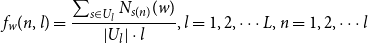
We observe that words under investigation exhibit distinct position–frequency distribution patterns. To find possible regularities in these patterns, we cluster words according to the patterns of their position–frequency distributions (relative frequency in this case). Figure 1 illustrates the position–frequency distribution of the top-3 most populated clusters on length 15 sentences (the sentence length with most sentences in our corpora), where the frequencies of each cluster is obtained by averaging the frequencies of all words in that cluster. From Figure 1, we observe that the frequencies of words at two ends of sentences deviate significantly from the general patterns in the middle of the sentences.
Figure 1. The position–frequency distribution of top-3 most populated word clusters on length 15 sentences.
In addition, we use multiple linear regression to model the relationship between word frequency and position-related factors, including sentence length and absolute position. To produce more reliable results, we make careful selection of words. A word is eligible for this experiment if it appears in more than 10 sub-corpora and the average of its frequencies (the maximum frequency excluded) in all positions in the sub-corpora is greater than 10. There are 3931 words that meet this criterion. Selected words are then examined of their position–frequency relationship by predicting the relative word frequency
 $f (n,l )$
(obtained by Equation (10)) with model:
$f (n,l )$
(obtained by Equation (10)) with model:
 \begin{equation} f(n, l)=\alpha _{0}+\alpha _{1} l+\alpha _{2} n+\alpha _{3} b_{1}+\alpha _{4} b_{2}+\alpha _{5} b_{3}+\alpha _{6} d_{1}+\alpha _{7} d_{2}+\alpha _{8} d_{3} \end{equation}
where
 $l$
represents sentence length and
$l$
represents sentence length and
 $n$
stands for the absolute position of the word in the sentence.
$n$
stands for the absolute position of the word in the sentence.
 $b_1$
,
$b_1$
,
 $b_2$
, and
$b_2$
, and
 $b_3$
refer to the first three positions at the beginning of the sentence, while
$b_3$
refer to the first three positions at the beginning of the sentence, while
 $d_1$
,
$d_1$
,
 $d_2$
, and
$d_2$
, and
 $d_3$
represent the last three positions at the end of the sentence. For example, if a word occurs at the first place of the sentence, then
$d_3$
represent the last three positions at the end of the sentence. For example, if a word occurs at the first place of the sentence, then
 $b_1=1$
,
$b_1=1$
,
 $b_2=b_3=d_1=d_2=d_3=n=0$
.
$b_2=b_3=d_1=d_2=d_3=n=0$
.
 $\alpha _0\dots \alpha _8$
are the coefficients of the regression model.
$\alpha _0\dots \alpha _8$
are the coefficients of the regression model.
We applied this model (Equation (12)) to all words selected and came up with following results: The regression models of 98.3% of the words are of
 $p\lt 0.05$
in F-test. The average
$p\lt 0.05$
in F-test. The average
 $R^2$
of models of selected words is 0.6904
$R^2$
of models of selected words is 0.6904
 $\pm$
0.1499 (the error term is standard deviation, same in the following sections); the percentages of models with
$\pm$
0.1499 (the error term is standard deviation, same in the following sections); the percentages of models with
 $p\lt 0.05$
in t-test on eight independent variables are 73.11%, 72.87%, 91.43%, 74.26%, 65.94%, 69.22%, 80.82%, and 88.25%, respectively, with an average of 76.97%
$p\lt 0.05$
in t-test on eight independent variables are 73.11%, 72.87%, 91.43%, 74.26%, 65.94%, 69.22%, 80.82%, and 88.25%, respectively, with an average of 76.97%
 $\pm$
8.46%.
$\pm$
8.46%.
The above results show that about 69% of the variance in word frequency is determined by these position-related factors we considered. The frequency of about 77% of the words is significantly affected by these factors. The third position at the beginning of a sentence affects the least (about 66% of the words), while the first position at the beginning of a sentence affects the most (over 90% of the words) which is followed by the last position at the end of a sentence.
The F-test and t-test results of the model described in Equation (12) suggest that the position-related independent variables significantly influence the frequency of words. In what follows, to dive deeper into the influence of individual factors, we single out each factor to investigate it’s influence on word frequency.
4.1.2. The influence of sentence length on word frequency
Is the frequency of a word affected by the length of the sentence it occurs in? Or, is there a difference in the probability of a word appearing in shorter sentences versus longer sentences? To answer this question, we calculate the frequency of words in each sub-corpus. To counter the influence of the number of sentences in each sub-corpus on word frequency, we evaluate
 $p_w (l )$
: the relative frequency of word
$p_w (l )$
: the relative frequency of word
 $w$
, that is, the absolute frequency of word
$w$
, that is, the absolute frequency of word
 $w$
divided by the number of sentences of length
$w$
divided by the number of sentences of length
 $l$
with following formula:
$l$
with following formula:
 \begin{equation} p_{w}(l)=\frac{\sum _{s \in U_{l}} \sum _{n=1}^{l} N_{s(n)}(w)}{\left |U_{l}\right | \cdot l}, \quad l=1,2, \cdots L \end{equation}
where
 $|U_l|$
is the number of sentences in sub-corpus
$|U_l|$
is the number of sentences in sub-corpus
 $U_l$
. With this formula, we accumulate the number of the occurrences of word
$U_l$
. With this formula, we accumulate the number of the occurrences of word
 $w$
in all absolute positions. The remaining variables in Equation (13) have the same meanings as the corresponding variables in Equation (10).
$w$
in all absolute positions. The remaining variables in Equation (13) have the same meanings as the corresponding variables in Equation (10).
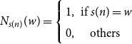
Figure 2 illustrates the relationship between the relative frequency
 $p_w (l )$
and sentence length for six words. We can see from the figure that words exhibit different sentence length–frequency relationships: the relative frequency of some words show positive correlation with sentence length, while the opposite is true for other words; some words demonstrate linear-like sentence length–frequency relationship, while others show quadratic-like relationship.
$p_w (l )$
and sentence length for six words. We can see from the figure that words exhibit different sentence length–frequency relationships: the relative frequency of some words show positive correlation with sentence length, while the opposite is true for other words; some words demonstrate linear-like sentence length–frequency relationship, while others show quadratic-like relationship.
Figure 2. The relationship between sentence length and word frequency.

Figure 3. The relationship between absolute position and word frequency.
For the reliability of our results, in the following statistical analysis, we consider only sub-corpora with enough sentences, ranging from 5 to 36 in length. A word occurring over 10 times in each sub-corpus is eligible for this experiment. There are 21,459 words that meet this criterion.
We use quadratic polynomial regression to examine the relationship between word frequency and sentence length. The mean coefficient of determination
 $R^2$
of resulting models is 0.4310
$R^2$
of resulting models is 0.4310
 $\pm$
0.2898; We use the sign of Pearson’s correlation coefficient to roughly estimate the influence of sentence length on word frequency and observed that the Pearson’s
$\pm$
0.2898; We use the sign of Pearson’s correlation coefficient to roughly estimate the influence of sentence length on word frequency and observed that the Pearson’s
 $r$
of 58.92% of the words are positive.
$r$
of 58.92% of the words are positive.
In summary, relative word frequency is thus significantly correlated with sentence length. When other variables disregarded, sentence length alone account for 43% of the variability of the word frequency, and the relative frequency of about 60% of the words increases with sentence length.
4.1.3. The influence of absolute position on word frequency
In this section, we investigate the effect of absolute position on word frequency. Figure 3 illustrates the relationship between the frequency of “said” and “in” and their absolute positions in sentences. It can be seen in the figure that curves at two ends of sentences are significantly different from curves at middle positions. The frequency curves of some words (e.g., “said”) head downward at the beginning of sentences followed by a sharp rise at ending positions, while the curves of other words (e.g., “in”) rise at the beginning positions followed by a downward trend at ending positions. However, the curves of both kinds of words stretch smoothly in middle positions. Besides, for each selected word, similar position–frequency curves are observed over sub-corpora of different sentence lengths. The frequency of words
 $f_w^{U_l} (n )$
are calculated as:
$f_w^{U_l} (n )$
are calculated as:
 \begin{equation} f_{w}^{U_{l}}(n)=\sum _{s \in U_{l}} N_{s(n)}(w), k \in [1,2, \cdots l] \end{equation}
where the variables at the right-hand side of the equation are of the same meanings as in Equation (10).
Based on our observation of the relationship between the frequency of words and their absolute positions, we test for outliers when examining the relationship between the frequency and the absolute position of words with following procedure:
-
Step 1. In each sub-corpus
 $U_l$
, we examine the relationship between the frequency of words (calculated with Equation (14)) and their absolute positions by quadratic polynomial regression;
$U_l$
, we examine the relationship between the frequency of words (calculated with Equation (14)) and their absolute positions by quadratic polynomial regression; -
Step 2. Based on the results in Step 1, we calculate the standard deviation of the residual between the word frequency predicted by the model and the observed frequency;
-
Step 3. If the difference between the observed and predicted frequency of a word at a position is three times greater than the standard deviation obtained in Step 2, we consider the frequency of the word at that position to be an outlier and exclude it from the regression in the next step;
-
Step 4. After outliers being removed, we rerun the polynomial regression and calculate the Pearson correlation coefficient on the remaining data.

The final results obtained from the whole procedure includes the outliers detected in Step 3 and the regression results in Step 4.
Taking the word frequency of “run” in sub-corpus
 $U_{15}$
as an example, the main idea of the procedure is to determine whether the data points to be detected fall between the upper and lower curves demonstrated in Figure 4. If it does not fall in-between, it is considered an outlier.
$U_{15}$
as an example, the main idea of the procedure is to determine whether the data points to be detected fall between the upper and lower curves demonstrated in Figure 4. If it does not fall in-between, it is considered an outlier.
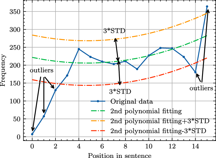
Figure 4. Quadratic polynomial regression with outlier detection.
For the reliability of the results in this experiment, we select sentences and words following the criteria detailed in Section 3.3.3. The experiment is performed based on the selected 3947 words with following results: the mean
 $R^2$
of the polynomial regression is 0.3905
$R^2$
of the polynomial regression is 0.3905
 $\pm$
0.07027; the percentage of Pearson’s correlation coefficient greater than 0 is 61.95%. As for outlier test, 4.96%
$\pm$
0.07027; the percentage of Pearson’s correlation coefficient greater than 0 is 61.95%. As for outlier test, 4.96%
 $\pm$
5.39% of the words at position 0, 1.57%
$\pm$
5.39% of the words at position 0, 1.57%
 $\pm$
1.45% at position 1, 0.92%
$\pm$
1.45% at position 1, 0.92%
 $\pm$
0.8% at position 2, 0.6%
$\pm$
0.8% at position 2, 0.6%
 $\pm$
0.46% at position -3, 4.62%
$\pm$
0.46% at position -3, 4.62%
 $\pm$
3.84% at position -2, and 12.55%
$\pm$
3.84% at position -2, and 12.55%
 $\pm$
1.25% at position -1 are outliers with an average of 4.20%
$\pm$
1.25% at position -1 are outliers with an average of 4.20%
 $\pm$
0.72%.
$\pm$
0.72%.
In summary, over 4% of the frequencies at two ends of sentences deviate from the overall pattern of frequency distribution of middle positions. Besides, 39.05% of the variance in the word frequency is caused by absolute position, and the frequency of 62% of the words increases with their absolute position.
In the section to follow, we investigate the position-related factors that affect the frequency of bigrams. We do this first by briefly discussing the possible factors may influence the frequency of bigrams and developing a formula to calculate bigram frequency. We then study the influence of these factors with statistical methods.
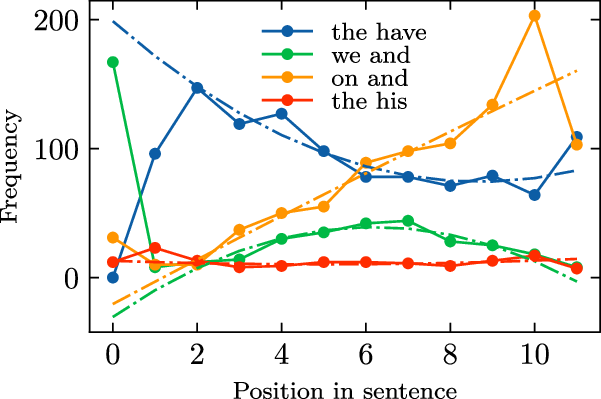
Figure 5. The relationship between relative position and bigram frequency in length 15 sub-corpora.
4.2. The influence of position-related factors on bigram frequency
We use bigram to model the co-occurrence frequency of two-word sequences to better understand the correlation between any two words modeled by self-attention mechanism. From a linguistic point of view, there are semantic and syntactic correlations between words in a sentence, which are reflected as beyond-random-level co-occurrence probability of words. Intuitively, this high co-occurrence probability caused by correlations can be modeled with relative positions between words. For example, “between A and B” is an expression where “between” and “and” should have a higher-than-chance co-occurrence probability when the relative position is 2. As for “if
 $\ldots$
then
$\ldots$
then
 $\ldots$
,” “if” and “then” won’t co-occur quite often when the relative position is small (e.g., 1, 2 or 3). Some bigrams (such as “what about”) occur more frequently at the beginning rather than the end of sentences. Also, some bigram, such as “and then,” should appear more frequently in longer sentences than in shorter ones. We believe that following position-related factors influence the frequency of a bigram: (1) the relative position of the two words that make up a bigram; (2) the absolute position of a bigram in a sentence; (3) whether a bigram occurs at the beginning or the end of a sentences; and (4) the sentence length. Therefore, we determine the relative frequency of a bigram
$\ldots$
,” “if” and “then” won’t co-occur quite often when the relative position is small (e.g., 1, 2 or 3). Some bigrams (such as “what about”) occur more frequently at the beginning rather than the end of sentences. Also, some bigram, such as “and then,” should appear more frequently in longer sentences than in shorter ones. We believe that following position-related factors influence the frequency of a bigram: (1) the relative position of the two words that make up a bigram; (2) the absolute position of a bigram in a sentence; (3) whether a bigram occurs at the beginning or the end of a sentences; and (4) the sentence length. Therefore, we determine the relative frequency of a bigram
 ${fr}_{w_1,w_2}(k,n,l)$
consisting of word
${fr}_{w_1,w_2}(k,n,l)$
consisting of word
 $w_1$
and
$w_1$
and
 $w_2$
in sentences
$w_2$
in sentences
 $s=s_1s_2\cdots s_n$
at position
$s=s_1s_2\cdots s_n$
at position
 $n$
and
$n$
and
 $n+k$
with the following formula:
$n+k$
with the following formula:
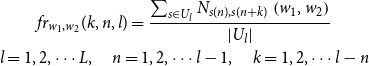 \begin{equation} \begin{gathered} f r_{w_{1}, w_{2}}(k, n, l)=\frac{\sum _{s \in U_{l}} N_{s(n), s(n+k)}\left (w_{1}, w_{2}\right )}{\left |U_{l}\right |} \\ l=1,2, \cdots L, \quad n=1,2, \cdots l-1, \quad k=1,2, \cdots l-n \end{gathered} \end{equation}
where
 $U_l$
is the sub-corpus consisting of sentences of length
$U_l$
is the sub-corpus consisting of sentences of length
 $l$
;
$l$
;
 $N_{s_n,s_{n+k}}(w_1,w_2)$
is a binary function which indicates whether word
$N_{s_n,s_{n+k}}(w_1,w_2)$
is a binary function which indicates whether word
 $w_1$
and
$w_1$
and
 $w_2$
appear at position
$w_2$
appear at position
 $n$
and
$n$
and
 $n+k$
in sentence
$n+k$
in sentence
 $s$
, which is formalized as:
$s$
, which is formalized as:
 \begin{equation} N_{s(n), s(n+k)}\left (w_{1}, w_{2}\right )=\left \{\begin{array}{lc} 1, & \text{ if } s(n)=w_{1} \text{ and } s(n+k)=w_{2} \\ 0, & \text{ others } \end{array}\right. \end{equation}
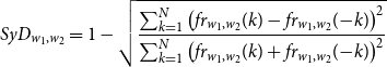
Figure 5 illustrates the frequency distributions of four bigrams over absolute positions in sub-corpus
 $U_{15}$
, where the relative position of each bigram is –2. The dotted lines in Figure 5 represent the predicted bigram frequencies by linear regression. We observe that the patterns of position and frequency distributions of bigrams are similar to that of words: regular patterns of distribution in middle positions and idiosyncratic patterns at both ends of sentences.
$U_{15}$
, where the relative position of each bigram is –2. The dotted lines in Figure 5 represent the predicted bigram frequencies by linear regression. We observe that the patterns of position and frequency distributions of bigrams are similar to that of words: regular patterns of distribution in middle positions and idiosyncratic patterns at both ends of sentences.
4.2.1. The joint influence of position-related factors on bigram frequency
To determine whether the frequency of a bigram is influenced by position-related factors, we use multiple linear regression models to examine the relationship between bigram frequency and following position-related factors: (1) sentence length; (2) relative position; and (3) absolute position; (4) whether a bigram occurs at the beginning or the end of sentences. If the model fits the data well, we consider the frequency of a bigram is influenced by these factors.
For each bigram, we perform a multiple linear regression which predicts
 $fr$
(the relative frequency of a bigram) to examine the influence of these position-related factors on the frequency of bigrams:
$fr$
(the relative frequency of a bigram) to examine the influence of these position-related factors on the frequency of bigrams:
 \begin{equation} fr=\alpha _0+\alpha _1l+\alpha _2n+\alpha _3k+\alpha _4b_1+\alpha _5b_2+\alpha _6b_3+\alpha _7d_1+\alpha _8d_2+\alpha _9d_3 \end{equation}
where
 $l$
is the sentence length,
$l$
is the sentence length,
 $n$
refers to the absolute position of a bigram, and
$n$
refers to the absolute position of a bigram, and
 $k$
is the relative position. The remaining coefficients and variables on the right-hand side of Equation (17) are of the same meanings as those in Equation (12).
$k$
is the relative position. The remaining coefficients and variables on the right-hand side of Equation (17) are of the same meanings as those in Equation (12).
For the reliability of our results, in the following statistical analysis, we select sentences and bigrams following the criteria detailed in Section 3.3.3. With 4172 selected bigrams, we arrived at following results of multiple linear regression:
The mean coefficient of determination
 $R^2$
of 4172 regression models is 0.5589
$R^2$
of 4172 regression models is 0.5589
 $\pm$
0.2318; the
$\pm$
0.2318; the
 $p$
-values of 99.59% bigram models are lower than 0.05 in F-test; The percentage of models with
$p$
-values of 99.59% bigram models are lower than 0.05 in F-test; The percentage of models with
 $p\lt 0.05$
in t-tests of 10 parameters are 89.85%, 72.51%, 67.50%, 63.97%, 87.56%, 78.12%, 61.12%, 72.89%, 81.77%, and 88.27%, respectively, with an average of 76.35%
$p\lt 0.05$
in t-tests of 10 parameters are 89.85%, 72.51%, 67.50%, 63.97%, 87.56%, 78.12%, 61.12%, 72.89%, 81.77%, and 88.27%, respectively, with an average of 76.35%
 $\pm$
9.86%.
$\pm$
9.86%.
The result that 99.59% of bigram’s regression models are with
 $p$
-values less than 0.05 in F-test indicates that the linear regression models are valid, and the frequency of almost all selected bigrams are significantly affected by these position-related factors. The result of coefficients of determination indicates that nearly 56% of the variance in frequency is due to these position-related factors.
$p$
-values less than 0.05 in F-test indicates that the linear regression models are valid, and the frequency of almost all selected bigrams are significantly affected by these position-related factors. The result of coefficients of determination indicates that nearly 56% of the variance in frequency is due to these position-related factors.
The frequencies of about 76% of bigrams are significantly influenced by these factors, among which the first position at the beginning of a sentence and the last position at the end of a sentence affect more bigrams than other coefficients which is similar to the case of word frequency.
In what follows, to dive deeper into the influence of individual factors, we single out each factor to investigate it’s influence on bigram frequency.
4.2.2. The influence of sentence length on bigram frequency
To study the relationship between the frequency of bigrams and the length of sentences where the bigrams occur, we examine the frequency of bigrams in sub-corpora with following formula:
 \begin{equation} f r_{w_{1}, w_{2}}(l)=\frac{\sum _{s \in U_{l}} \sum _{n=1}^{l-1} \sum _{k=1}^{l-n} N_{s(n), s(n+k)}\left (w_{1}, w_{2}\right )}{\left |U_{l}\right | \cdot (l-1) !}, l=1,2, \cdots L \end{equation}
The variables in Equation (18) are of the same meanings as those in Equation (15);
 $ |U_l |\cdot (l-1 )!$
in denominator is the number of bigrams can be extracted from sub-corpus
$ |U_l |\cdot (l-1 )!$
in denominator is the number of bigrams can be extracted from sub-corpus
 $U_l$
. This formula is derived by accumulating
$U_l$
. This formula is derived by accumulating
 $n$
and
$n$
and
 $k$
in Equation (15).
$k$
in Equation (15).
Figure 6 illustrates diverse patterns of frequency distribution for six bigrams over sentence lengths, calculated with Equation (18). From the figure, we observe both rising and falling curves with varying rate of change.
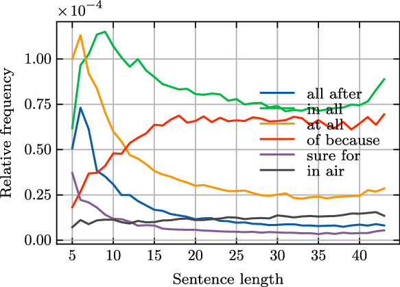
Figure 6. The relationship between sentence length and bigram frequency.
Based on Equation (18), we examined the relationship between the frequency
 $fr$
of bigrams and length
$fr$
of bigrams and length
 $l$
of sentences with quadratic polynomial regression. For the reliability of results, we select sentences of length 6 to 36. The mean coefficient of determination of resulting models is 0.7631
$l$
of sentences with quadratic polynomial regression. For the reliability of results, we select sentences of length 6 to 36. The mean coefficient of determination of resulting models is 0.7631
 $\pm$
0.2355. As for the linear correlation between bigram-frequency and sentence length, the Pearson’s
$\pm$
0.2355. As for the linear correlation between bigram-frequency and sentence length, the Pearson’s
 $r$
s of 60.68% of the bigrams are greater than 0. That is, when other variables disregarded, about 76% of the variability in bigram frequency is caused by variation of sentence length, and the frequency of about 61% of the bigrams increases with the sentence length.
$r$
s of 60.68% of the bigrams are greater than 0. That is, when other variables disregarded, about 76% of the variability in bigram frequency is caused by variation of sentence length, and the frequency of about 61% of the bigrams increases with the sentence length.
4.2.3. The influence of relative position on bigram frequency
Long-distance decay (i.e., as the relative position between words extends, the strength of correlation between words decreases accordingly) is considered a desirable property of current PE schemas (Yan et al. Reference Yan, Deng, Li and Qiu2019). In this study, we investigate this property in detail.
To study the relationship between the relative position and frequency of bigrams, we first need to specify our calculation method of bigram frequency. We care only the relationship between the relative position of bigrams and their frequency and dispense with other factors. Therefore, we accumulate the variables
 $n$
and
$n$
and
 $l$
in Equation (15) and keep only the variable
$l$
in Equation (15) and keep only the variable
 $k$
to obtain the marginal distribution of
$k$
to obtain the marginal distribution of
 ${fr}_{w_1,w_2}$
. And we model the relationship between
${fr}_{w_1,w_2}$
. And we model the relationship between
 ${fr}_{w_1,w_2}$
and
${fr}_{w_1,w_2}$
and
 $k$
with this marginal distribution. Relative position (distance)
$k$
with this marginal distribution. Relative position (distance)
 $k$
is restricted by sentence lengths, for example, bigram “if then (4)” (i.e., the “
$k$
is restricted by sentence lengths, for example, bigram “if then (4)” (i.e., the “
 $\ldots$
if X X X then
$\ldots$
if X X X then
 $\ldots$
” pattern) occur only in sentences of lengths greater than 5. Therefore, the maximum relative position
$\ldots$
” pattern) occur only in sentences of lengths greater than 5. Therefore, the maximum relative position
 $k$
is
$k$
is
 $l-1$
in a sentence of length
$l-1$
in a sentence of length
 $l$
. Obviously, the smaller the value of
$l$
. Obviously, the smaller the value of
 $k$
, the more sentences contain the k-skip-bigram. To cancel out the influence of the number of sentences available, we divide the absolute frequency of a bigram with the number of sentences containing that bigram:
$k$
, the more sentences contain the k-skip-bigram. To cancel out the influence of the number of sentences available, we divide the absolute frequency of a bigram with the number of sentences containing that bigram:
 \begin{equation} f r_{w_{1}, w_{2}}(k)=\frac{\sum _{s \in U}\left (\sum _{n=1}^{|s|-k} N_{s(n), s(n+k)}\left (w_{1}, w_{2}\right )\right )/(|s|-k)}{\sum _{l=k+1}^{L}\left |U_{l}\right |} \end{equation}
where all right-hand-side variables are of the same meanings as those in Equation (15).
Figure 7 illustrates the relationship between the frequency of four bigrams and their relative position. It can be seen in the figure that the frequencies of the bigrams are affected by relative positions: bigram frequencies at shorter relative positions differ significantly from those at longer relative positions.
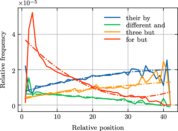
Figure 7. The relationship between relative position and bigram frequency.
With the same method used in Section 4.1.3, we examined the relationship between the frequency of bigrams
 $fr$
and relative position
$fr$
and relative position
 $k$
with quadratic polynomial regression and performed outlier detection at the same time.
$k$
with quadratic polynomial regression and performed outlier detection at the same time.
The results of the regression analysis are as follows: the mean
 $R^2$
of the models is 0.5357
$R^2$
of the models is 0.5357
 $\pm$
0.2561, and the Pearson’s
$\pm$
0.2561, and the Pearson’s
 $r$
s between
$r$
s between
 $fr$
and
$fr$
and
 $k$
of 33.33% of the bigrams are greater than 0. Besides, 47.72% of the outliers are observed at relative position
$k$
of 33.33% of the bigrams are greater than 0. Besides, 47.72% of the outliers are observed at relative position
 $k=1$
, followed by 17.63% at
$k=1$
, followed by 17.63% at
 $k=2$
, 5.31% at
$k=2$
, 5.31% at
 $k=3$
and less than 5% at remaining relative positions.
$k=3$
and less than 5% at remaining relative positions.
That is, when other variables disregarded, about 54% of the variability of bigram frequency is explained by the relative position variation. The frequency of about one-third of bigrams increases with the increasing relative position. Besides, for nearly half of the bigrams, their frequency at relative position
 $k=1$
deviates significantly from the overall pattern of their frequency distribution at other relative positions.
$k=1$
deviates significantly from the overall pattern of their frequency distribution at other relative positions.
Some studies pay attention to the symmetry of positional embedding, and a property indicates that the relationship between two positions is symmetric. Wang et al. (Reference Wang, Shang, Lioma, Jiang, Yang, Liu and Simonsen2021) claim that BERT with APE does not show any direction awareness as its position embeddings are nearly symmetrical. In the next section, we therefore take a statistical approach to study the symmetry in our corpora.
4.2.4. The symmetry of frequency distributions of bigrams over relative position
Symmetry here can be interpreted in this paper as the fact that swapping the positions of two words in a bigram does not cause a significant change in their co-occurrence frequency. We can statistically define the symmetry as:
 \begin{equation} E(p(k)-p({-}k))=0 \end{equation}
where
 $p (k )$
is the probability of a bigram at relative position
$p (k )$
is the probability of a bigram at relative position
 $k$
and
$k$
and
 $E ({\cdot})$
is the mathematical expectation.
$E ({\cdot})$
is the mathematical expectation.
For a bigram consisting of words A and B, we call it symmetric if, for any value of
 $k$
, the probability of its occurrence in form “
$k$
, the probability of its occurrence in form “
 $A\ X_1X_2\cdots X_k\ B$
” is equal to the probability of its occurrence in form “
$A\ X_1X_2\cdots X_k\ B$
” is equal to the probability of its occurrence in form “
 $B\ Y_1Y_2\cdots Y_k\ A$
” in sentences. Intuitively, if words A and B are not correlated in sentences, they can randomly occur at any position, so their co-occurrence frequency should be symmetric over relative positions. However, word order of an expression is an important semantic device which cannot be reversed without changing the meaning of the expression. If two constituent words of a bigram are associated, then there should exist a special relative position. That is, the frequency distribution of a bigram over relative position should be asymmetric.
$B\ Y_1Y_2\cdots Y_k\ A$
” in sentences. Intuitively, if words A and B are not correlated in sentences, they can randomly occur at any position, so their co-occurrence frequency should be symmetric over relative positions. However, word order of an expression is an important semantic device which cannot be reversed without changing the meaning of the expression. If two constituent words of a bigram are associated, then there should exist a special relative position. That is, the frequency distribution of a bigram over relative position should be asymmetric.
According to Equation (20), if the frequency distribution of a bigram over relative positions is symmetric, then
 ${fr}_{w_1,w_2} (k )-{fr}_{w_1,w_2} ({-}k )\ (k\gt 0)$
should be small. Therefore, we conduct pairwise statistical tests on the distributions
${fr}_{w_1,w_2} (k )-{fr}_{w_1,w_2} ({-}k )\ (k\gt 0)$
should be small. Therefore, we conduct pairwise statistical tests on the distributions
 ${fr}_{w_1,w_2} (k )$
and
${fr}_{w_1,w_2} (k )$
and
 ${fr}_{w_1,w_2} ({-}k )$
with following procedure:
${fr}_{w_1,w_2} ({-}k )$
with following procedure:
For all selected bigrams
 $(w_1,w_2)$
, we first test the normality of
$(w_1,w_2)$
, we first test the normality of
 ${fr}_{w_1,w_2} (k )$
and
${fr}_{w_1,w_2} (k )$
and
 ${fr}_{w_1,w_2} ({-}k )$
, if both of them follow normal distribution, we then perform paired-sample t-test on them. Otherwise, we turn to Wilcoxon matched-pairs signed rank test.
${fr}_{w_1,w_2} ({-}k )$
, if both of them follow normal distribution, we then perform paired-sample t-test on them. Otherwise, we turn to Wilcoxon matched-pairs signed rank test.
The test result shows that 10.31% of the bigrams are of
 $p$
-value greater than 0.05, indicating that
$p$
-value greater than 0.05, indicating that
 ${fr}_{w_1,w_2} (k )$
and
${fr}_{w_1,w_2} (k )$
and
 ${fr}_{w_1,w_2} ({-}k )$
are not significantly different. In other words, the frequency distribution over relative position of around 90% of the selected frequent bigrams can not be considered symmetric.
${fr}_{w_1,w_2} ({-}k )$
are not significantly different. In other words, the frequency distribution over relative position of around 90% of the selected frequent bigrams can not be considered symmetric.
To measure the degree of symmetry of the frequency distribution of bigrams over relative position, we define the symmetry index as:
 \begin{equation} SyD_{w_{1}, w_{2}}=1-\sqrt{\frac{\sum _{k=1}^{N}\left (f r_{w_{1}, w_{2}}(k)-f r_{w_{1}, w_{2}}({-}k)\right )^{2}}{\sum _{k=1}^{N}\left (f r_{w_{1}, w_{2}}(k)+f r_{w_{1}, w_{2}}({-}k)\right )^{2}}} \end{equation}
where
 ${fr}_{w_1,w_2}(k)$
is the relative frequency as in Equation (19), and
${fr}_{w_1,w_2}(k)$
is the relative frequency as in Equation (19), and
 $N$
is the maximum relative position. Since there are significantly fewer sentences containing bigrams with larger relative position than those with lower relative position, we consider only bigrams of relative position lower than 36 for the reliability of our statistical results. Equation (21) measures the proportion of the difference between two distributions in the sum of the two distributions. The value of symmetry index ranges from 0 to 1. The closer the symmetry index is to 1, the smaller the difference between the two distributions; the closer the symmetry index is to 0, the larger the difference between the two distributions.
$N$
is the maximum relative position. Since there are significantly fewer sentences containing bigrams with larger relative position than those with lower relative position, we consider only bigrams of relative position lower than 36 for the reliability of our statistical results. Equation (21) measures the proportion of the difference between two distributions in the sum of the two distributions. The value of symmetry index ranges from 0 to 1. The closer the symmetry index is to 1, the smaller the difference between the two distributions; the closer the symmetry index is to 0, the larger the difference between the two distributions.
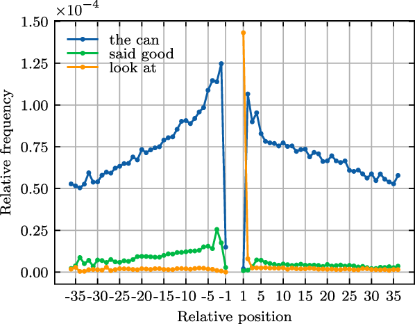
Figure 8. Relative position–frequency distribution of three bigram with different degrees of symmetry.
Three bigrams with intuitively different degrees of symmetry are shown in Figure 8, and their symmetry indices are 0.9267, 0.5073, and 0.0121, respectively. As can be seen in the figure, the symmetry index we defined in Equation (21) matches our intuition of symmetry. In order to reliably investigate the degree of symmetry of the frequency distribution of bigrams, we selected those frequent bigrams and calculate their symmetry indices with Equation (21). We use frequency as the criterion of selection: bigrams with frequency over 1000 are selected for our experiment. We set this threshold frequency based on the following considerations: given the size of the corpus and lengths of sentences, the relative position between two words in a sentence ranges from -43 to + 43, that is, there are nearly 100 relative positions. As a rule of thumb, if we expect the mean frequency of bigrams on each position to be over 10, then the total frequency of each bigram should be no less than 1000. With this criterion, we obtained 200,000 bigrams.
The result of this experiment shows that the mean symmetry index value of selected bigrams is 0.4647
 $\pm$
0.1936. That is, on average, the difference between the frequency of bigrams over positive and negative relative position account for about 46% of the total frequency.
$\pm$
0.1936. That is, on average, the difference between the frequency of bigrams over positive and negative relative position account for about 46% of the total frequency.
We also calculated the Pearson correlation coefficients between the symmetry index and the frequency and the logarithmic frequency of the selected bigrams, with results of 0.0630 and 0.2568, respectively. The results suggest that the degree of symmetry of a bigram’s frequency distribution over relative position is weakly but positively correlated with its frequency. The higher the frequency, the higher the degree of symmetry, which may be consistent with the fact that the function words all have high frequency and most of them have no semantic correlation with other words.
In what follows, we show through a case study that the distribution patterns of bigrams over relative positions contain linguistic information, which, we believe, will inspire the development of language models which are expected to make better use of linguistic information.
4.2.5. Grammatical information from the distribution patterns of bigrams
According to the distributional hypothesis (Harris Reference Harris1954), the meaning of a word can be represented by the context in which it occurs. And the context of a word in a corpus is generally considered to be a set consisting of all sentences in which the word occurs. Currently, in order to obtain the contextual representation, one more common approach is to feed the sentences in this set into a language model one by one. In fact, we can also use another approach: using context models, such as k-skip-n-gram, to extract relations between the focus word and its context in this set and then input the extracted relations to a language model. If a language model (e.g., BERT, GPT, ELMo, Peters et al. Reference Peters, Neumann, Iyyer, Gardner, Clark, Lee and Zettlemoyer2018) can capture the relationships between words and their contexts, then the results of applying the two methods should be the same.
In what follows, with a case study, we demonstrate that more linguistic information can be obtained by a language model if the second method is considered.
We examined the frequency distribution of the bigrams consisting of the nominative and genitive forms of English personal pronouns over relative position and observed that they have similar patterns of distribution (see Figure 9).
Figure 9. The frequency distribution of bigrams consisting of nominative and genitive variant of English pronouns over relative position.
We then calculated paired Pearson’s correlation coefficients between the distribution curves of the seven pronouns in Figure 9, resulting in a minimum of 0.8393 and a maximum of 0.9866, with a mean of 0.9414
 $\pm$
0.0442. However, when all bigrams considered, the mean value is 0.1641
$\pm$
0.0442. However, when all bigrams considered, the mean value is 0.1641
 $\pm$
0.3876, and the mean of the absolute value of Pearson’s correlation coefficient is 0.3478
$\pm$
0.3876, and the mean of the absolute value of Pearson’s correlation coefficient is 0.3478
 $\pm$
0.2372. This result shows the distribution patterns personal-pronoun bigrams over relative position resemble each other with above-average similarity.
$\pm$
0.2372. This result shows the distribution patterns personal-pronoun bigrams over relative position resemble each other with above-average similarity.
As can be seen in Figure 9, the symmetry indices of the seven bigrams are close to each other, recording 0.4738, 0.3267, 0.4563, 0.3803, 0.5033, 0.4269, and 0.6282, respectively, with an average of 0.4565
 $\pm$
0.0890.
$\pm$
0.0890.
The result suggests that more grammatical information can be obtained if a Transformer-based model can organize the self-attention weights of the same bigram scattered over multiple positions in the attention matrix into a distribution of attention weights.
The similarity between the distribution patterns shown in Figure 9 also suggests that distribution patterns contain grammatical information. If the co-occurrence frequency distributions of bigrams over relative position are fed to or learned spontaneously by neural network language models, models can thus learn richer grammatical information.
In the next section, we investigate the influence of the absolute position of bigrams on their frequency in sentences of different lengths.
4.2.6. The influence of absolute position on bigram frequency
Our analysis in Section 4.2 suggests that bigrams have their preferred absolute positions. Next, we examine the relationship between the frequency and the absolute position of bigrams. We determine
 $f_{w_1,w_2}^{U_l} (n )$
: the frequency of a bigram consisting of word
$f_{w_1,w_2}^{U_l} (n )$
: the frequency of a bigram consisting of word
 $w_1$
and
$w_1$
and
 $w_2$
in sub-corpus
$w_2$
in sub-corpus
 $U_l$
at position
$U_l$
at position
 $n$
with:
$n$
with:
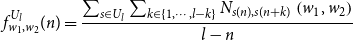 \begin{equation} f_{w_{1}, w_{2}}^{U_{l}}(n)=\frac{\sum _{s \in U_{l}} \sum _{k \in \{1, \cdots,l-k\}} N_{s(n), s(n+k)}\left (w_{1}, w_{2}\right )}{l-n} \end{equation}
where the variables at the right-hand side of the equation have the same meaning as their corresponding variables in Equation (15). The distribution function
 $f_{w_1,w_2}^{U_l} (n )$
is derived from a ternary function
$f_{w_1,w_2}^{U_l} (n )$
is derived from a ternary function
 ${fr}_{w_1,w_2} (k,n,l )$
by fixing
${fr}_{w_1,w_2} (k,n,l )$
by fixing
 $l$
and accumulating
$l$
and accumulating
 $k$
in sub-corpus
$k$
in sub-corpus
 $U_l$
. The relative position
$U_l$
. The relative position
 $k$
that can be accumulated at the absolute position
$k$
that can be accumulated at the absolute position
 $n$
are
$n$
are
 $1, 2,\dots, l-n$
, with a total of
$1, 2,\dots, l-n$
, with a total of
 $l-n$
values. The effect of differences in the number of relative positions on the frequency of bigrams is linguistically meaningless and beyond the scope of our study. Therefore, the quotient obtained by dividing the cumulative result by
$l-n$
values. The effect of differences in the number of relative positions on the frequency of bigrams is linguistically meaningless and beyond the scope of our study. Therefore, the quotient obtained by dividing the cumulative result by
 $l-n$
, which eliminates the effect of the difference in the number of relative positions on the bigram frequency, is the bigram frequency influenced by absolute position that we are interested in.
$l-n$
, which eliminates the effect of the difference in the number of relative positions on the bigram frequency, is the bigram frequency influenced by absolute position that we are interested in.
In sentences of different lengths, even bigrams with the same absolute position have different positions relative to the whole sentence. Therefore, to determine the relationship between the frequency and the absolute frequency of bigrams in the whole corpus, the examinations are first conducted in each sub-corpus. Then the number of sentences in each sub-corpus is used as the weight in the weighted average calculation. This procedure is the same as the examination of the relationship between the frequency and absolute position of words.
We use quadratic polynomial regression to examine the relationship between the frequency and absolute position of 19,988 bigrams, followed by outlier detections. The mean
 $R^2$
of quadratic polynomial regression models at the middle positions of sentences is 0.4807
$R^2$
of quadratic polynomial regression models at the middle positions of sentences is 0.4807
 $\pm$
0.0815. The percentage of outliers at first and last three positions are 4.93%
$\pm$
0.0815. The percentage of outliers at first and last three positions are 4.93%
 $\pm$
5.16%, 1.37%
$\pm$
5.16%, 1.37%
 $\pm$
1.17%, 0.41%
$\pm$
1.17%, 0.41%
 $\pm$
0.33%, 2.26%
$\pm$
0.33%, 2.26%
 $\pm$
1.89%, 4.82%
$\pm$
1.89%, 4.82%
 $\pm$
4.00%, and 5.58%
$\pm$
4.00%, and 5.58%
 $\pm$
6.19%, respectively, with an average of 3.23%
$\pm$
6.19%, respectively, with an average of 3.23%
 $\pm$
0.55%. The mean percentage of outliers at first and last positions is 5.26%
$\pm$
0.55%. The mean percentage of outliers at first and last positions is 5.26%
 $\pm$
1.00%, that is, the frequency of over 5% of the bigrams at two ends of sentences in all sub-corpora deviate far from the overall distribution patterns. After outliers being removed, for 41.10% of the bigrams, the Pearson correlation coefficients between the absolute position and frequency of bigrams is greater than 0, indicating that the frequency of about 40% of the bigrams increases as the absolute position increases.
$\pm$
1.00%, that is, the frequency of over 5% of the bigrams at two ends of sentences in all sub-corpora deviate far from the overall distribution patterns. After outliers being removed, for 41.10% of the bigrams, the Pearson correlation coefficients between the absolute position and frequency of bigrams is greater than 0, indicating that the frequency of about 40% of the bigrams increases as the absolute position increases.
These results show that the frequencies of some bigrams at the beginning and end of sentences are significantly different from the overall pattern of their frequency distribution elsewhere in the sentence. The relationship between the frequency and the position of bigrams can be modeled with quadratic polynomials. About 48% of the variability of bigram frequency can be accounted for by the variation of absolute position, and the frequency of around 41% of the bigrams increases with their absolute position.
For the reliability of our statistical results, in previous experiments, we excluded bigrams and words which occur on average less than 10 times at each sampling point. This treatment determines that analyses in previous experiments present conclusions merely hold for frequent words and bigrams. In the next section, we perform brief statistical analysis on the relationship between the frequency and the position of words in different frequency bands to gain some knowledge about the position–frequency distribution of previously excluded words.
4.3. The position distribution of low-frequency words
To obtain consistent position–frequency distributions of low-frequency words is a tricky attempt due to their sparse occurrence in the corpus. As such, it is unfeasible to count the frequency of a low-frequency word at every position. As a workaround, we simplify this issue by roughly dividing all positions into three groups, namely the beginning, the middle, and the end of a sentence, where the beginning refers to the first three positions of a sentence, the end refers to the last three positions of a sentence, and the middle refers to the rest positions. We then calculate the relative frequency of each word at these three “positions” and calculate the average of these relative frequencies for the words within each frequency band separately.
As can be seen in Figure 10, words in lower frequency bands show higher frequency at the beginning positions of sentences, while there is little difference in the frequency of words in higher frequency bands at three positions. Words in frequency bands in-between show higher frequency at the end positions of sentences. That is, words of different chance of occurrence exhibit different patterns of position distribution. It is thus suggested that the conclusions we made in previous sections cannot be extrapolated to words or bigrams of lower chance of occurrence.
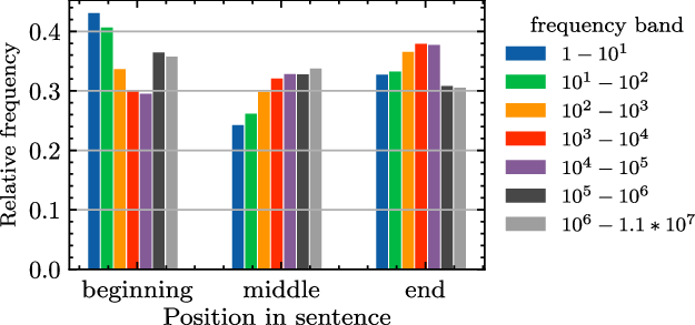
Figure 10. Position–frequency distribution of words in different frequency bands.
5. Discussion
In this study, correlations between language units in sentences are modeled as their co-occurrence frequency. The examination on the correlation between language units is carried out by multiple linear regression and quadratic polynomial regression. The results show that both word and bigram frequency have complex relationships with position-related factors. Relative position, absolute position (including the beginning and ending positions), and sentence length all have significant effects on word frequency and bigram frequency. Our results suggest that, when developing a PE model, it is desirable to explicitly take these factors into account. However, the input layers of current Transformer-based models have not taken advantage of these factors. Another idea is to include additional layers after multi-head self-attention layer to give the Transformers the ability to computationally derive richer position information.
The results of Shaw et al. (Reference Shaw, Uszkoreit and Vaswani2018) and Rosendahl et al. (Reference Rosendahl, Tran, Wang and Ney2019) have shown that models adopting relative position achieve better performance than absolute position in downstream tasks. The word order within chunks is fixed and of particular importance, while the order and distance between chunks are relatively free. Therefore, models based on RPE can directly model word chunks, while models based on absolute position require further processing. Besides, by investigating the frequency of bigrams over relative position, our study suggests that patterns of frequency distribution of bigrams entail rich grammatical information which apparently also requires further processing to be adequately captured by the current language models.
Our study also revealed that sentence length has a significant influence on the frequency of words and bigrams. However, sentence length is currently a neglected factor as no currently popular model encodes sentence lengths explicitly. Takase and Okazaki (Reference Takase and Okazaki2019) achieved improved performance in a language generation task by incorporating sentence length information explicitly, which is an indirect evidence of the usefulness of sentence length.
By comparing 13 variants of position embedding/encoding schemas, Wang et al. (Reference Wang, Shang, Lioma, Jiang, Yang, Liu and Simonsen2021) concluded that APEs are more suitable for classification tasks, while relative embeddings perform better for span prediction tasks. We believe that a model built with a relative positioning schema can directly encode the correlation between words and is therefore more conducive to span prediction tasks. Absolute positioning schemas do not directly model the correlation between words and are therefore not good for span prediction tasks. However, classification tasks require global information of the input text, and absolute positioning schemas obviously encode more global position information than relative ones.
In named entity recognition (NER) tasks, Yan et al. (Reference Yan, Deng, Li and Qiu2019) proposed a direction- and distance-aware attention mechanism which improved the task performance. According to the results of our study, 90% of the bigrams have asymmetric frequency distribution patterns over relative positions; thus, an awareness of the direction of relative position is necessary as it improves the accuracy of prediction.
Some studies input the syntactic structures of sentences (e.g., dependency trees, Shiv and Quirk Reference Shiv and Quirk2019; Wang et al. Reference Wang, Wang, Chen, Wang and Kuo2019a) rather than simple positional information to the model, hoping that neural network language models can make use of the human-labeled grammatical information. However, this attempt only made marginal improvement to task performance. Based on the results of this study, this problem may be caused by two factors: first, neural network language models may fail to make good use of syntactic structure information as obtaining syntactic information from these structures requires additional processing; second, not all kinds of position information is needed for every task, and more-than-necessary types of position information do not necessarily lead to better performance. Intuitively, the structure of an input sentence can provide models with more information about the relationship between words. However, according to the report by Wang et al. (Reference Wang, Wang, Chen, Wang and Kuo2019a), the improvement brought by incorporating syntactic structure is only marginal. This result suggests that the model fails to fully utilize the position information encoded by syntactic structures. Or, in other words, the structural information of sentences is not as important to models as it is to linguists.
Several works have found linguistic knowledge in neural network language models, such as subject–verb agreement and reflexive dependencies in BERT’s self-attention mechanism (Lin, Tan, and Frank Reference Lin, Tan and Frank2019), parse tree distances in BERT (Manning et al. Reference Manning, Clark, Hewitt, Khandelwal and Levy2020), and singular/plural relationships (Lakretz et al. Reference Lakretz, Kruszewski, Desbordes, Hupkes, Dehaene and Baroni2019; Goldberg Reference Goldberg2019). However, it is not yet clear in what forms these linguistic information exist in a corpus and how they are learned by language models. The similarity of the frequency distribution of bigrams consisting of the nominative and genitive forms of English pronouns observed in this paper suggests that this linguistic knowledge exists in the pattern of joint frequency distribution of linguistic units.
By introducing additional interactions between query, key, and relative position embeddings to self-attention mechanism, Huang et al. (Reference Huang, Liang, Xu and Xiang2020) improved the performance of BERT. According our results on sentence length, absolute position, and relative position, we speculate that the improved performance brought by these proposed additional interactions are associated with these position-related factors. Based on the results of this work and previous studies, a reasonable hypothesis is that different NLP tasks require different kinds of position information. Although various forms of position information can be derived from each other, it has not been explicitly reflected in the models’ architectures.
The results also show that the frequency of words is related to factors including absolute position and sentence length and whether they occur at two ends of sentences. In addition to the above factors, the inter-word relationship is also affected by relative position. Since current neural network language models do not autonomously derive one variable from another, we need to feed the information explicitly to the model. For example, in sentence “Tom and Jerry is in inarguably one of the most celebrated cartoons of all time,” according to the conclusion made in this study, multiple types of information should be explicitly feed into neural network language models: for focus word “Tom,” we need to explicitly feed all of the following quantities to neural network language models: its absolute position (encoded as 0); its being at the beginning of the sentence (encoded as 1, 0, 0); its absence from the end of the sentence (encoded as 0, 0, 0); its relative position from all other words in the sentence (i.e., –1 from “and”, –2 from “Jerry”,
 $\ldots$
, –13 from “time”) and its sentence length 14. These factors are not yet considered holistically in recent Transformer-based architectures.
$\ldots$
, –13 from “time”) and its sentence length 14. These factors are not yet considered holistically in recent Transformer-based architectures.
Our large-corpus-based study suggests that the inter-word relationship is rather complicated. The co-occurrence frequency of about one-third of the bigrams increases with the relative position, while the co-occurrence frequency of other two-thirds take the opposite. That is, it is not possible to conceive the inter-word relationship with a single law. It is also found in previous studies that the way sentences are processed by BERT during training will bring about unexpected properties to sentences. For example, Wang et al. (Reference Wang, Shang, Lioma, Jiang, Yang, Liu and Simonsen2021) discovered that over-long sentences when truncated either at the beginning or the end will endow the APE with the property of translation invariance. Our study suggests that the truncation procedure systematically affects the precision of the estimation of the context of word occurrence.
For the reliability of the results, this study focus merely on words or bigrams the occurrence of which surpass set threshold. The investigation of the position–frequency distribution of words in different frequency bands suggests that the excluded words of lower chance of occurrence show different patterns of position distribution from words of higher chance of occurrence. We, therefore, suggest that the conclusions arrived by studying words and bigrams with more occurrences cannot be directly extrapolated to words or bigrams with lower chance of occurrence. A great proportion of less frequent words are tokenized by current popular neural network language models into few Word-pieces. The vocabularies of these Word-pieces are determined jointly by tokenization algorithms and downstream tasks, which suggests that the relationship between the low-frequency words and position-related factors should be studied jointly with tokenization algorithms and downstream tasks (Park et al. Reference Park, Lee, Jang and Jung2020; Vasiu and Potolea Reference Vasiu and Potolea2020).
6. Conclusion
To analyze in detail the position-related factors that affect the correlation between language units, we studied the relationships between the frequency and the position of words and bigrams.
We first examined the influence of absolute position (including the beginning and ending positions), relative position, and sentence length on the frequency of language units with multiple linear regression models. 98.3% of the models of words have
 $p$
-values less than 0.05 in F-tests with a mean
$p$
-values less than 0.05 in F-tests with a mean
 $R^2$
of 0.6904
$R^2$
of 0.6904
 $\pm$
0.1481; 99.59% of the models of bigrams have
$\pm$
0.1481; 99.59% of the models of bigrams have
 $p$
-values less than 0.05 in F-tests with a mean
$p$
-values less than 0.05 in F-tests with a mean
 $R^2$
of 0.5589
$R^2$
of 0.5589
 $\pm$
0.2318. The F-test results suggest that the multiple linear regression models are effective in modeling the relationships between the frequency and position of words and bigrams. Our results also show that about 70% of the variance in word frequency and about 56% of the variance in bigram frequency are caused by these position-related factors.
$\pm$
0.2318. The F-test results suggest that the multiple linear regression models are effective in modeling the relationships between the frequency and position of words and bigrams. Our results also show that about 70% of the variance in word frequency and about 56% of the variance in bigram frequency are caused by these position-related factors.
We studied then the influence of single position-related factor on language unit frequency with quadratic polynomial regression and observed that:
1. The average
 $R^2$
of the models describing the relationship between word frequency and sentence length is 0.4310
$R^2$
of the models describing the relationship between word frequency and sentence length is 0.4310
 $\pm$
0.2898. The weighted average
$\pm$
0.2898. The weighted average
 $R^2$
of the models representing the relationship between the absolute position and the frequency of words is 0.3905
$R^2$
of the models representing the relationship between the absolute position and the frequency of words is 0.3905
 $\pm$
0.07027. Besides, over 3% of the word frequencies at first and last three positions of sentences in all sub-corpora deviate far from the overall patterns of distribution. Our results also show that the variability of absolute position and sentence length each account for about 40% of the variation of word frequency, and the presence of words at two ends of sentences affects the word frequency as well.
$\pm$
0.07027. Besides, over 3% of the word frequencies at first and last three positions of sentences in all sub-corpora deviate far from the overall patterns of distribution. Our results also show that the variability of absolute position and sentence length each account for about 40% of the variation of word frequency, and the presence of words at two ends of sentences affects the word frequency as well.
2. The average
 $R^2$
of the quadratic polynomial regression models describing the relationship between bigram frequency and sentence length is 0.7631
$R^2$
of the quadratic polynomial regression models describing the relationship between bigram frequency and sentence length is 0.7631
 $\pm$
0.2355. The average
$\pm$
0.2355. The average
 $R^2$
of the quadratic polynomial regression models describing the relationship between bigram frequency and relative position is 0.5357
$R^2$
of the quadratic polynomial regression models describing the relationship between bigram frequency and relative position is 0.5357
 $\pm$
0.2561. As for the relationship between the frequency and relative position, the Pearson correlation coefficients of 33.33% of the bigrams are greater than 0. The average
$\pm$
0.2561. As for the relationship between the frequency and relative position, the Pearson correlation coefficients of 33.33% of the bigrams are greater than 0. The average
 $R^2$
of the polynomial regression models describing the relationship between bigram frequency and absolute position is 0.4807
$R^2$
of the polynomial regression models describing the relationship between bigram frequency and absolute position is 0.4807
 $\pm$
0.0815. Over 5% of the bigram frequencies at first and last three positions of sentences in all sub-corpora deviate far from the overall patterns of frequency distributions. Overall, when examined separately, the variability of absolute position, sentence length and relative position each account for 76%, 54%, and 48% of the variation of the frequency of bigrams, and the presence of bigrams at two ends of sentences slightly affects their frequency as well.
$\pm$
0.0815. Over 5% of the bigram frequencies at first and last three positions of sentences in all sub-corpora deviate far from the overall patterns of frequency distributions. Overall, when examined separately, the variability of absolute position, sentence length and relative position each account for 76%, 54%, and 48% of the variation of the frequency of bigrams, and the presence of bigrams at two ends of sentences slightly affects their frequency as well.
3. With paired statistical tests, we examined the symmetry of frequency distribution of bigrams over positive and negative relative positions. The frequency distribution of 10.31% of the bigrams are symmetric over positive and negative relative positions.
4. We examined the frequency distributions of bigrams consisting of the nominative and genitive forms of English personal pronouns over relative position and observed similar patterns of distribution, suggesting that the frequency distributions of bigrams carry grammatical information.
In conclusion, based on our examinations of the frequency of words and bigrams, we show that the correlations between words are affected not only by absolute and relative position but also by sentence length and whether the words occur at two ends of a sentence. However, these factors are not yet explicitly encoded by current PE architectures.
Acknowledgments
Research on this paper was funded by National Social Science Foundation of China (20AYY021), Science Foundation of Beijing Language and Culture University (supported by “the Fundamental Research Funds for the Central Universities”) (20YJ140010), and the MOE Project of Key Research Institute of Humanities and Social Sciences at Universities in China (22JJD740018).


 Open access