


1 Lightweight structures with fibre-reinforced plastics: Chances and challenges of structural design
Fibre-reinforced plastics (FRP) increasingly turn out to have a powerful impact for resource efficient products in the future due to their function integration capabilities. To reduce weight in future electric cars, for example, FRP are currently developed further for use in so-called structural batteries (Asp Reference Asp2013), bearing mechanical load and serving as an electric energy storage at the same time. This kind of function integration could allow for a considerable weight reduction by eliminating the ‘structurally parasitic’ (Asp Reference Asp2013), separate batteries. Furthermore, especially when used in safety-critical applications like aerospace, the material’s suitability for function integration allows for sophisticated security features, like the integration of structural health monitoring capabilities via so-called smart layers (Capezzuto et al. Reference Capezzuto, Ciampa, Carotenuto, Meo, Milella and Nicolais2010). These layers exhibit different properties when subjected to different kinds of impact loads, for example, luminescence or altered magnetic behaviour. Last, additive manufacturing technologies (Kussmaul et al. Reference Kussmaul, Könen, Türk, Spierings, Klahn, Ermanni, Zogg and Meboldt2016) allow for integrated positioning and fixation elements and precise adaptation of structural optimisation results, among others.
In any case, today as in the future, FRP structures still have to fulfil stiffness and strength requirements equally to their function integration targets. However, structural design for composites remains a challenge, considering manufacturing and cost requirements (Schürmann Reference Schürmann2007) while at the same time keeping the complex engineering design in mind (Michaeli, Huybrechts & Wegener Reference Michaeli, Huybrechts and Wegener1995) with a typically large number of mutually dependent parameters (Klein, Malezki & Wartzack Reference Klein, Malezki, Wartzack, Weber, Husung, Cascini, Cantamessa, Marjanovic and Rotini2015). Thus, sophisticated computer aided engineering tools and approaches (Vajna et al. Reference Vajna, Weber, Zeman, Hehenberger, Gerhard and Wartzack2018) have been developed, among them Altair OptiStruct and mfk Composite Designer (mfkCODE), a comparison of which was presented in Völkl, Franz & Wartzack (Reference Völkl, Franz and Wartzack2018a). A decisive factor for effective lightweight designs is fibre orientation according to load path trajectories (Schürmann Reference Schürmann2007), as a faulty orientation can significantly decrease both stiffness (Klein, Witzgall & Wartzack Reference Klein, Witzgall, Wartzack, Marjanović, Štorga, Pavković and Bojčetić2014) and strength results (Reuschel & Mattheck Reference Reuschel and Mattheck1999). Various methods exist for fibre orientation optimisation, reaching from continuous fibre angle optimisation (Bruyneel & Fleury Reference Bruyneel and Fleury2002) to genetic algorithms (Bardy, Legrand & Crosky Reference Bardy, Legrand and Crosky2012) and load path computation (Kelly, Reidsema & Lee Reference Kelly, Reidsema and Lee2011). Within a new approach for structured laminate design (Klein et al. Reference Klein, Malezki, Wartzack, Weber, Husung, Cascini, Cantamessa, Marjanovic and Rotini2015) developed at Friedrich-Alexander University Erlangen-Nuremberg, the computer aided internal optimisation (CAIO) method by Mattheck (Mattheck Reference Mattheck1997; Reuschel & Mattheck Reference Reuschel and Mattheck1999; Mattheck & Tesari Reference Mattheck and Tesari2000) is used. This method showed up as very effective reaching lightweight goals, especially concerning stiffness optimisation (Reuschel & Mattheck Reference Reuschel and Mattheck1999; Völkl et al. Reference Völkl, Franz and Wartzack2018a). Its main principle – aligning fibre orientations with principal normal stress trajectories – is also in accordance with certain optimality derivations (Luo & Gea Reference Luo and Gea1998). However, for use in advanced laminate design, questions still remain open (Völkl, Franz & Wartzack Reference Völkl, Franz, Wartzack, Ermanni, Meboldt, Wartzack, Krause and Zogg2018b). In the following section, the method is introduced in detail and both strengths and open questions are discussed.
2 The CAIO method: State of the art and questions raised
2.1 Overview and working principle
Being inspired by tree and bone growth, the CAIO method simulates internal optimisation of trees (Reuschel & Mattheck Reference Reuschel and Mattheck1999). By aligning fibre orientations with principal normal stress trajectories, its intention is to reduce failure-critical shear stresses as far as possible.
After setting up a finite element analysis (Figure 1), a first calculation is conducted with an initial material orientation, which can be unidirectional (Mattheck & Tesari Reference Mattheck and Tesari2000), arbitrary (Reuschel & Mattheck Reference Reuschel and Mattheck1999) or, as proposed by the authors (Völkl et al. Reference Völkl, Klein, Franz and Wartzack2018), isotropic material. The emerging principal normal stress trajectories are then used for orientation of the main orthotropic axis in each element. For this purpose, the principal normal stress eigenvector with the largest absolute eigenvalue should be used (Spickenheuer Reference Spickenheuer2014). From this new fibre orientation state, a new stress state emerges, which is used as input for the next CAIO iteration until shear stresses are ‘sufficiently’ reduced. The method depends on an appropriately fine mesh to allow proper local adaptation of orientation. The aim of the method is to obtain high-stiffness, high-strength lightweight structures (Reuschel & Mattheck Reference Reuschel and Mattheck1999). For certain shear weak types of orthotropic materials, mathematical studies indicate that alignment of fibre orientations with principal normal stress trajectories indeed provides the stiffest structure (Gea & Luo Reference Gea and Luo2004).
However, aligning fibre orientations with principal normal stress trajectories is not always unambiguous, as stress states that do not provide a single but two (for plane stress state) largest principal normal stresses can occur. This shows up in regions of heavily multiaxial stresses, as demonstrated in Figure 2.

Figure 1. Overview of the CAIO method adapted from Reuschel & Mattheck (Reference Reuschel and Mattheck1999).

Figure 2. Multiaxial stress states leading to ambiguous fibre trajectories. (a) Region with unique largest principal normal stresses and (b) problematic region. Adapted from Völkl et al. (Reference Völkl, Franz, Wartzack, Ermanni, Meboldt, Wartzack, Krause and Zogg2018b).
From experience, it is known that such multiaxial stress states typically appear in real-world examples with complicated geometries and load cases. While it seems obvious to use several layers in the finished part, within the CAIO method, it is not clear how to deal with such stress states. Solutions have been proposed – simply keeping the method as above (with maximum absolute principal normal stress eigenvalues, called ‘maximum absolute’ in the following) or searching for finite elements within proximity, which exhibit unambiguous fibre directions and adapting their orientation (Klein Reference Klein2017) (called ‘proximity search’ from here on). In Klein et al. (Reference Klein, Malezki, Wartzack, Weber, Husung, Cascini, Cantamessa, Marjanovic and Rotini2015), the CAIO method is further modified for multi-layer capabilities (ML-CAIO), which is discussed at the end of the main part of this contribution.
2.2 Questions raised
For practical, early phase applications, a fast convergence of an optimisation method is desirable in order to test and evaluate different prototypes (Vajna et al. Reference Vajna, Weber, Zeman, Hehenberger, Gerhard and Wartzack2018). Most computational effort during structural optimisation methods is needed for solving finite element analysis and calculating gradients (if used). Reducing the amount of required finite element solutions saves, besides computational effort, time. It makes the method more applicable in early phases through the possibility of performing more optimisation runs or optimising more parts. Because the CAIO method is a heuristics-based algorithm which needs no further information like gradients, the amount of needed finite element solutions is equal to the number of iterations. To evaluate the applicability, in this contribution, the convergence behaviour of the CAIO method will be scrutinised and evaluated for various demonstrators, ranging from simple geometry and load case to more sophisticated parts.
Moreover, the CAIO break criterion is still not properly defined in clear terms. To quantify the idea of ‘sufficiently reduced’ shear stresses, this break criterion is thoroughly formulated – and alternatives will be presented and compared.
Third, this contribution deals with non-unique principal normal stress trajectories (ambiguous fibre orientations), which occur in finite elements showing highly multiaxial stress states as discussed above. The significance of the problem and the different methods to tackle it are discussed in terms of stiffness and convergence behaviour which builds on a distinguished contribution at the first symposium Lightweight Design in Product Development, Zurich (Völkl et al. Reference Völkl, Franz, Wartzack, Ermanni, Meboldt, Wartzack, Krause and Zogg2018b).
The CAIO method as originally defined can only handle one single layer, thereby obviously omitting the great lightweight capabilities when using laminates with several different layers. Therefore, in the last part, an overview is given when multi-layer CAIO as introduced by Klein et al. (Reference Klein, Malezki, Wartzack, Weber, Husung, Cascini, Cantamessa, Marjanovic and Rotini2015) is applied. In this contribution, new examinations of the multi-layer CAIO are conducted: Is stiffness behaviour improved, and to what amount? What about the influence of deviations from nominal, optimised fibre angles as calculated by the CAIO method?
3 Discussing the application of the CAIO method
3.1 Convergence and break criteria scrutiny
To get insights into convergence behaviour of the CAIO method in various situations, three representative demonstrators were chosen and optimised by the CAIO method.
The first demonstrator is a notched plate under plane loading with strongly multiaxial stress states around the notch. The second demonstrator, a mounting bracket, exceeds the plate by a more complicated geometry and torsion as its load case. In composite structure experts’ knowledge, sure enough, this demonstrator is not a favourable part to be manufactured from FRP. However, it is chosen to demonstrate the method’s behaviour under adverse conditions. Finally, the third demonstrator, a b-pillar, is a complicatedly shaped sheet part under oblique bending load similar to Völkl et al. (Reference Völkl, Klein, Franz and Wartzack2018), which stands for close to real-world conditions. Figure 3 presents the three demonstrators.

Figure 3. Introduction of demonstrators: (a) notched plate, (b) mounting bracket and (c) b-pillar.
3.1.1 Resulting fibre orientations of the CAIO method
Figure 4 shows the results of the optimisation procedure applied to the notched plate (first and tenth iterations). Fibre orientations are shown as black lines within the elements, and the fibre angle to the given coordinate system is indicated by colour. For all demonstrators, a carbon-fibre-reinforced plastic material model was used (in the iterations with anisotropic material).

Figure 4. Optimised fibre orientations for the notched plate.
The fibre orientations align properly with the load path, bearing the bending load case resulting from the vertical force (Figure 3) and the tension force on the right border of the part. The angle difference along the neutral fibre from bending is quite high, which runs approximately horizontally along the middle of the demonstrator. Here, the transition from tension to compression appears. Overall fibre paths run smoothly.

Figure 5. Optimised fibre orientations for the mounting bracket.
Figure 5 shows the resulting fibre orientations of the method for the mounting bracket under torsion load (one layer). While in the first iteration distinct segments are recognisable, after 10 iterations, the result converges (see the following section) to a quite chaotic steady state – which is unsatisfactory and thus discussed further in the later part of this contribution.

Figure 6. Optimised fibre orientations for the b-pillar.
The resulting fibre layout of the b-pillar in Figure 6 exhibits several similarly aligned regions corresponding to tension and compression regions because of the bending load case applied. There are some regions of fibre orientation direction change; however, overall fibre trajectories run smoothly, as for the notched plate.
3.1.2 Convergence measures and break criteria
After presenting the visual results of the CAIO method in the previous section, quantitative quality criteria have to be found to evaluate both improvement through optimisation and convergence behaviour. Three criteria were studied: (1) shear stress reduction, emerging from Reuschel & Mattheck (Reference Reuschel and Mattheck1999) claiming reduction of shear stresses; (2) overall strain energy reduction, which in turn stands for increased stiffness, as a typical stiffness measure in topology optimisation; (3) a lack of change in local fibre angles (Spickenheuer Reference Spickenheuer2014), which is only suitable for convergence behaviour, not for quality estimation. These are specified as follows:
(1) For shear stress reduction within this optimisation, no clear mathematical description of a global convergence criterion is given in literature. While in Reuschel & Mattheck (Reference Reuschel and Mattheck1999) and Mattheck & Tesari (Reference Mattheck and Tesari2000) the convergence criterion is defined as reduction of shear stresses which has to be evaluated manually, in Reuschel (Reference Reuschel1999) and Spickenheuer (Reference Spickenheuer2014), the convergence criterion is defined more clearly as reduction of the maximum shear stress. How to consider multiple integration points within state-of-the-art shell elements, or even multiple layers, is not described. Klein (Reference Klein2017) introduces a convergence criterion based on the mean shear stresses of all elements. Based on this, the authors propose a simplified criterion, a sum of element shear stresses, using the following measure: After any iteration with anisotropic material, calculate stress tensors for all finite elements; transform each of these to the respective fibre coordinate system (
 $x$-axis is fibre direction, $z$ is element normal and $y$ is perpendicular); use the absolute value of shear stresses in the $XY$ plane (hypothesis: approximately plane stress state) of each element and sum these up over the whole part (all finite elements). Like this, the measure is suitable to quantify an overall amount of shear stresses – which are to be reduced during the course of iterations.
(2) For strain energy, the sum of individual strain energy of all elements is used.
(3) For change in local fibre angles, the median of all fibre angle differences between two iterations is used. Thus, it is possible to specify the change in angles with 50% of angle differences happening above and below, respectively, preventing strong outliers from having too much impact. However, to be comprehensive, the maximum change in angles for each iteration is always given in the following studies as well.


Sufficiently, specified ‘small’ change during iterations of these convergence criteria will be used as break criterion to stop the optimisation, if possible. The following convergence scrutiny shall reveal whether the respective convergence criteria are suitable for this purpose.
3.1.3 Convergence histories of the demonstrators
Figure 7(a)–(d) presents the convergence histories for each convergence criterion on all demonstrator parts.

Figure 7. Convergence histories for all demonstrators and convergence criteria.
The median angle differences between iterations in Figure 7(a) show a very smooth and steadily declining behaviour for all demonstrators. The optimisation of the mounting bracket (blue) exhibits higher median changes overall, which seems reasonable when the highly multiaxial stress states are taken into account. Convergence for all demonstrators can be observed at about 10 iterations (median lower than 0. 5°) – even if the overall geometrical intricacy of the demonstrators differs greatly, from a simple notched plate to a b-pillar.
Regarding the maximum angle differences of all elements (Figure 7b), it must be stated that for the more complicated demonstrators, mounting bracket and b-pillar, there always remain some elements in which the fibre direction flips 90° back and forth. However, for the b-pillar, this affects only 19 out of 18,639 elements (0.1%), for the mounting bracket 32 out of 3461 (∼1%) and none for the notched plate. This behaviour, thus, does not have much effect on stiffness overall (Figure 7d), yet makes this criterion completely unsuitable for CAIO convergence scrutiny.
The measure which is inspired by the original aim of CAIO’s inventors, shear stress reduction, provides a smooth, steadily declining behaviour for the notched plate and the b-pillar (Figure 7c). The scaling of this diagram sets maximum strain energy for each demonstrator part to 100%. For the notched plate, shear stresses are almost completely reduced; for the b-pillar, the reduction ends at about 50%. However, for the mounting bracket under torsion loading, there is even an increase in shear stresses in the second iteration. As this is not in line with a continuous shear stress reduction, a detailed scrutiny is provided.

Figure 8. Mounting bracket: Fibre orientations through iterations.
Figure 8 shows the fibre orientation angles in iterations 1–4 to observe the optimisation progress during the shear stress increase and in iteration 10 to have an idea about a later iteration’s behaviour. The heavily multiaxial stress states lead to many ±45°-orientations in the beginning (iteration 1); fibres are aligned with these and then provoke more or less chaotic behaviour and huge unsteady changes in orientations (2–3) until a sort of ‘chaos equilibrium’ is found (3–10), which is reflected in the overall iteration course above. This implies that a single-layer-based CAIO method is expectedly rather unsuitable for this overall heavy multiaxiality of stress states induced by loads, boundary conditions and geometry, which was also noted in Klein et al. (Reference Klein, Witzgall, Wartzack, Marjanović, Štorga, Pavković and Bojčetić2014).
Returning to criteria suitability for convergence behaviour scrutiny of the CAIO method, this could, with due care, imply the assumption that a stable convergence behaviour also indicates a suitability of the part for use of composite materials; however, in this empirical study, it allows the conclusion that this implementation of shear stress measurement can be a reasonable mean to check for convergence. For the given demonstrators, shear stress reduction convergence is reached at slightly more varying iteration numbers compared to the median angle difference (shear stress reduction: notched plate, 16 iterations; mounting bracket, around 17 iterations; b-pillar, 7 iterations – when less than 10% change between iterations is considered as convergence).
Strain energy sum (Figure 7(d)) behaves similarly to shear stress reduction. The scaling is the same as that for shear stresses (normed to maximum = 1). It becomes obvious that stiffness increase (strain energy reduction) is the largest for the mounting bracket during iterations (even though for this demonstrator the initial value is 90% as in the second iteration, strain energy goes up from the initially better design) and stiffness increase is dependent on the demonstrator. The overall calculated stiffness gain is around 10%–20%. From a convergence scrutiny point of view, in the beginning, a fast and huge reduction takes place, even though shear stresses might not have been reduced that much (less than 1% change in strain energy after 3 iterations for the notched plate, after 10 iterations for the mounting bracket and after 4 iterations for the b-pillar).
3.1.4 Subconclusion for convergence behaviour
The findings from the examples before imply that, first, median angle difference, shear stress reduction and strain energy sum all provide a reasonable measure for checking if the algorithm converged in principle. Just the maximum angle difference is unsuitable due to local ‘flipping’ effects. Strain energy seems to be the least conservative measure as it indicates convergence very early when shear stresses are not as much reduced as possible. This poses a disadvantage as shear stress reduction is crucial for good strength behaviour of composite structures (Schürmann Reference Schürmann2007; Knops Reference Knops2008). Median angle difference as a convergence criterion delivers a very uniform convergence duration behaviour (11 iterations for these very different demonstrators). However, shear stress reduction seems to take occasionally longer as just discussed. Thus, shear stress reduction seems to be a good criterion for measuring convergence behaviour as it is both reasonable from a physics point of view and shows smooth behaviour for suitable parts and boundaries/loads and, thus, maybe even serving as a counter-indicator (when a part is not suitable, convergence behaviour also seems to be bad). The number of needed iterations until convergence is dependent on the demonstrator and load case as well as of the convergence criterion. Nonetheless, the CAIO method is a very fast optimisation method, converging within few iterations. In some cases, the optimisation even converges in less than five iterations. The fast convergence coincides with the observations made in Spickenheuer (Reference Spickenheuer2014).
3.2 Ambiguous optimum trajectories – a stability issue?
From Figure 8, it became obvious that multiaxial stress states can lead to chaotic resulting designs. While from a numerical standpoint the results are understandable, the fibre layouts are not intuitive and manufacturable anymore. This section investigates the handling of such multiaxial stress states by using the ‘maximum absolute’ and ‘proximity search’ methods.
The ‘maximum absolute’ method always chooses the orientation of the biggest, absolute stress eigenvalue, i.e. the corresponding eigenvector, for orienting the fibres. Mathematically, this should lead to an optimal solution, but as demonstrated with the mounting bracket demonstrator or a pipe under torsional load (Klein Reference Klein2017), the stress states of many elements contain two nearly identical stress eigenvalues and, thus, ambiguous fibre trajectories to follow by the CAIO method.
In order to overcome the problems of the ‘maximum absolute’ method, the ‘proximity search’ method was developed by Klein (Reference Klein2017), which will be scrutinised deeper in the following section. For better understanding, the principle implementation of the ‘proximity search’ method is repeated here shortly: A pseudocode for its implementation is given in Algorithm 1. First, every element is checked for such an ambiguous stress state, i.e. for (nearly) equal principal normal stresses, which is also called an isotropic stress state in the following. An isotropy criterion has been introduced by Klein (Reference Klein2017) to detect this state, equation (1). The variable isotrTol defines the range of the quotient of two principal normal stresses in which an element’s stress state is considered isotropic.
 $$\begin{eqnarray}I_{\mathit{isoCrit}}=\frac{|\unicode[STIX]{x1D70E}_{I}|}{|\unicode[STIX]{x1D70E}_{II}|}~\in ~]1-\mathit{isotrTol},1+\mathit{isotrTol}[.\end{eqnarray}$$
If the isotropy criterion is true for an element’s stress state, the neighbour elements are checked for their stress states, pictured in Figure 9. If there is an element in the direct neighbourhood with a non-isotropic stress state, the fibre orientation of this element gets adopted. If all neighbour elements exhibit an isotropic stress state as well, the neighbours of the neighbours are checked consecutively until an element with unambiguous stress state is found. If there are no elements with unambiguous stress state, the CAIO method is cancelled and the initial stress state (first iteration with isotropic material) is chosen.

The aim of this method is to avoid chaotic, alternating fibre directions in areas with isotropic stress states. Moreover, the method should lead to more uniform layouts (Figure 9) which facilitate the transition to a patch design by resulting in bigger and more regular patches.
While the ‘maximum absolute’ method represents the optimal solution according to the original CAIO method (reduce shear stresses as far as possible), the ‘proximity search’ method intentionally deviates from the optimal solution with the focus of improving the subsequent steps in transforming the results into a practical laminate design. In the following section, the changes regarding stiffness, strength and convergence behaviour occurring from the use of the ‘proximity search’ method are presented for the three demonstrators.

Figure 9. Avoidance of alternating fibre directions using the “proximity search” method. Adapted from Völkl et al. (Reference Völkl, Franz, Wartzack, Ermanni, Meboldt, Wartzack, Krause and Zogg2018b).
3.2.1 Influence of the isotropy criterion on convergence behaviour
The isotropy tolerance is set to values between 0 and 0.9, where  $\mathit{isotrTol}=0$ means that there is no tolerance and therefore the maximum absolute principal stress is chosen as fibre direction. Accordingly, for a value of 0.9, many elements are detected as being isotropic. Figure 10 shows this relation for the three demonstrators.

Figure 10. Influence of isotropy criterion on number of isotropic elements over 20 iterations.
The mesh of the notched plate contains 4814 elements, of which even for the highest isotropic tolerance value (and in the first iteration), under 20% are affected by the proximity search method; similarly, this applies to the b-pillar. However, for the mounting bracket, at least about half of all 3461 elements are affected even when using low isotropic tolerance values.
Accordingly, Figure 11 depicts a rather small influence of the proximity search method on the convergence behaviour for the notched plate and the b-pillar and a large influence, however, on the convergence behaviour of the mounting bracket.
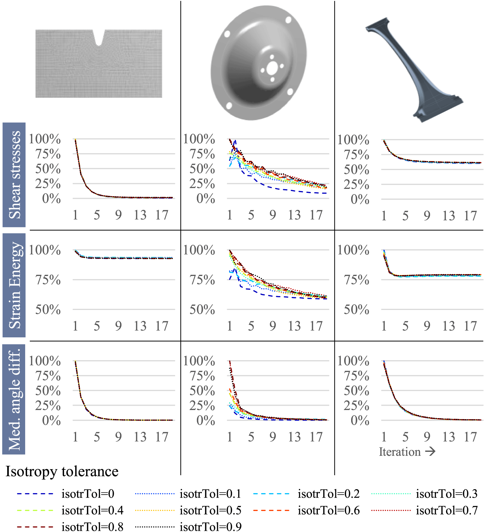
Figure 11. Influence of isotropy criterion on convergence behaviour of different convergence criteria over 20 iterations.
For the notched plate, all three criteria – shear stresses, strain energy and medium angle difference – remain largely unaffected as only some elements’ orientation is altered. As far as the mounting bracket is concerned, the following can be stated:
(i) Remaining shear stresses are higher for higher isotropy criterion values;
(ii) Strain energy is affected by the proximity search method during iterations but converges to a similar value (around 60% of initial strain energy) for all isotropy criterion values;
(iii) Median angle differences are larger at the beginning for higher isotropy criterion values but decrease quickly.
(iv) Overall, isotropy tolerance has a high influence on the first iteration. However, influence is much smaller in the next iterations when the number of isotropic elements decreases due to the CAIO optimisation.
For the b-pillar, the overall influence of the isotropy criterion on convergence behaviour is very small.
3.2.2 Subconclusion: Stress state dependent influence of the isotropy criterion on convergence behaviour
For heavily multiaxial stress states, a single-layer fibre orientation is ‘equally bad’ in any direction; thus, there is no significant stiffness difference; the shear stress reduction, however, is affected and the use of the proximity search method to improve (later stages) laminate patch regularity is, thus, not advisable. Under these circumstances, also the convergence behaviour is less controllable when using the proximity search method. In any case, for such stress states, the use of multiple layers is recommended, which is presented and discussed in the following section.
If regions of multiaxial stress states are limited, on the contrary, the isotropic tolerance has little influence on the criteria and their convergence behaviour. It thus can be used comfortably to simplify later-stage laminate layouts without losing too much stiffness.
3.3 Towards multi-layer optimisation
The original CAIO method is useful in giving an idea of force flow within a given geometry, thus providing trajectories along which fibres should ideally be placed. However, there are certain shortcomings when many regions of the geometry exhibit multiaxial stress states under the given load – and, therefore, most FRP optimisation approaches these days offer an elaborated multi-layer capability, e.g. Altair OptiStruct, ESAComp or approaches by Klein et al. (Reference Klein, Witzgall, Wartzack, Marjanović, Štorga, Pavković and Bojčetić2014) and Kussmaul, Zogg & Ermanni (Reference Kussmaul, Zogg and Ermanni2018). The approach by Klein et al. uses an altered CAIO method for multi-layer optimisation which is discussed in Klein (Reference Klein2017) and shortly described here: First, the (shell) geometry is split into multiple layers, each layer with equal thickness and adding up to a given overall thickness. The layers are modelled within finite element shell elements. Then, to optimise the fibre angles in each layer of every element, the stress tensor is calculated for every element layer via finite element analysis. The CAIO algorithm aligns the fibre trajectory with the direction of the maximum absolute principal stress in each layer. By iterating like in the original CAIO method for single-layer optimisation (first iteration isotropic material, then anisotropic), the optimised solution is found.
Convergence stability of this multi-layer CAIO method has not yet been studied intensively but is crucial for a successful application of a multi-layer optimisation routine. Therefore, in the following, two of the former demonstrator parts are investigated again with varying number of layers. The mounting bracket and b-pillar with their respective load cases introduced in Figure 3 are used for this scrutiny due to curved geometries and more complicated load cases. The notched plate is omitted as both geometry and forces are in-plane; thus, all layers of each element would simply take on the same orientation and, as such, no effect on convergence stability (or stiffness) can be expected which goes beyond single-layer scrutiny. The proximity search method is switched off ( $\mathit{isotrTol}=0$) to avoid its additional influence. The overall thickness of the demonstrators is set to 1 mm for the mounting bracket and 4 mm for the b-pillar. Each layer height is defined by overall thickness divided by layer number. The number of layers is raised from one to five and the convergence behaviour in terms of shear stresses, strain energy and median angle difference is studied. The results regarding stiffness and convergence for the multi-layer optimisation are presented in Figure 12.
3.3.1 Stiffness scrutiny
First, the stiffness is investigated by analysing the strain energy (mid row of Figure 12). The mounting bracket shows decreasing strain energy with increasing number of layers, which in turn indicates an increase in stiffness. The difference between the worst result (one layer) and the best result after the last iteration (four layers) is 14%. An especially steep increase in stiffness can be seen when shifting from one to two layers. Increasing the layer number further from two to three only provokes a small stiffness gain; after that, hardly any stiffness gain can be observed. The results of the optimisations of the b-pillar show a small increase of the stiffness between the optimisations with one and two layers. A steep stiffness increase cannot be observed until using three layers; after that, hardly any stiffness gain occurs, which is the same as that for the mounting bracket.

Figure 12. Influence of multiple layers on convergence behaviour.
The overall resulting difference of the strain energy between the optimisation with one layer and with five layers is considerable (29%), taking into account that the overall thickness does not change.
3.3.2 Subconclusion: Stiffness behaviour of multi-layer optimisations
More layers for optimisation (with constant overall laminate thickness) increase stiffness. The additional layers cover further loads reflected in principal stress directions apart from the maximum principal stress. For example, the mounting bracket demonstrator’s stiffness increases with the addition of a second layer as the multiaxial stresses in +45° and -45° direction can be covered. Another benefit of using multiple layers is the coverage of stresses varying with and being dependent on laminate thickness – multiple layers can cover different principal stress directions on the upper, middle and lower sides of the part. Exceeding a certain number of layers and thus thickness discretisation does not bring further benefit, indicating that occurring stresses have been covered appropriately.
3.3.3 Convergence scrutiny
Using Figure 12, the convergence behaviour is analysed like before, observing the sum of shear stresses, the sum of strain energy and median angle difference.
Regarding the summarised shear stresses of the mounting bracket, only small differences between one and multiple layers can be observed. While shear stresses in the first iterations increase with higher number of layers, the later convergence behaviour of the simulations is very similar. The final values differ by around 5%. The curves of the b-pillar behave similarly, except for the two-layer optimisation, which results in higher shear stresses. While the shear stresses of the b-pillar with one layer only show changes lower than 3% after 10 iterations, the one-layer optimisation of the mounting bracket maintains slight changes until the maximum number of iterations (due to ongoing variations in fibre orientations). Multi-layer optimisation results of the mounting bracket vary merely about 1% after the 10th iteration, thus providing a very good convergence behaviour.
The convergence behaviour of the strain energy shows a fast convergence behaviour for both the mounting bracket and the b-pillar. The only optimisation run taking more than 10 iterations for satisfactory convergence is the unsuitable one-layer optimisation of the mounting bracket.
The median angle differences of the mounting bracket optimisation runs with multiple layers show significantly lower start values compared to the one-layer optimisation; i.e. overall, angle changes in the beginning are much smaller. All optimisations converge after a maximum of 10 iterations. The last iteration’s median angle differences differ below 1% for all optimisations (one to five layers). In absolute numbers, the resulting value for the median of the angle differences in the last iteration is below 0. 1°. The graph for the b-pillar exhibits similar results. The start value of the median angle difference for the one-layer optimisation is higher than that for multiple layers. But the convergence behaviour and the trend of the curves is very similar for all numbers of layers. Compared to the mounting bracket, more iterations are needed until convergence. The resulting values differ very little.
3.3.4 Subconclusion: Convergence behaviour of multi-layer optimisations
Overall, the multi-layer CAIO method provides a stable convergence behaviour. When multiaxial stress states occur, multiple layers are favourable, which is reflected directly in convergence behaviour, which usually becomes more stable when increasing the number of layers (mounting bracket example). For the question which convergence criterion to choose, the response is actually that all three criteria seem suitable, as for the single-layer CAIO method. For one single layer, a clear pattern was identified that strain energy seems to be the least conservative measure of convergence as it converged first. Comparing multi-layer convergence behaviour now, that does not always hold true (e.g. b-pillar, strain energy and three layers). Yet, regarding all results, strain energy does not qualify as a cautious criterion guaranteeing full convergence. Angle differences could be used equally to the shear stresses because both seem a good choice: Convergence is indicated at similar iteration numbers independently of the layer number and of the criterion. However, shear stresses provide a physical meaning and, thus, are recommended.
3.3.5 Multi-layer results: Each layer in detail
Observing the decisive differences in convergence behaviour between one, two, three and occasionally four layers for the demonstrators, in the following, a detailed scrutiny of first iterations’ fibre layouts is conducted to further explain these differences.
Figure 13 shows the mounting bracket’s fibre layouts of two- (above) and three-layer optimisation (below): First, the result design with two layers is evaluated. The first layer results in curved fibre trajectories from the fixed supports to the holes where load is applied. The fibre angles are set at about 45° to the tangential direction of the mounting bracket. The mounting bracket’s fibre layout is divided into tension and compression sections. The fibre angles flip about 90° at the section borders, as indicated by abrupt colour changes. At the inner part of the sections, there also is an area where the fibre direction flips about 90°. In the inner ring close to the holes, the fibre directions mostly point to the loaded holes, indicating force flow.

Figure 13. Optimisation results with multiple layers for the mounting bracket.
In the outer areas close to the fixed supports, the second layer exhibits the same fibre orientations as the first layer. On the contrary, the load carrying regions between the holes and the supports show a change of the fibre angles. To analyse this inconsistency of angles between the two layers, Figure 14(a) is consulted. It indicates the fibre angle difference between the two layers. The comparison of the fibre angles of the different layers shows the influences of multiple layers on the optimisation more properly.
Figure 14(a) shows that the most elements in the load carrying area have a fibre angle difference  $\unicode[STIX]{x1D6E5}\unicode[STIX]{x1D6FC}$ of around 90°. Combined with the layer fibre angles of the first layer, a ±45° layup evolves, which is known as a proper laminate layup for shear stresses (Schürmann Reference Schürmann2007). At the tension-section and compression-section borders, elements with no difference in the fibre angles occur.

Figure 14. Fibre angle difference of the first and the second layers (a) of the optimised mounting bracket with two layers and (b) of the optimised b-pillar with four layers.
Observing the multi-layer optimisation of the mounting bracket with three layers in Figure 13, a behaviour similar to the two-layer optimisation is detected. The first layers of the three- and two-layer optimisation are almost the same, except for some artefacts (A). The third layer generally shows the same behaviour as that of the second layer of the two-layer optimisation. Yet, it contains more artefacts at the section borders and in the outer areas (B) where less stress occurs. The second layer resembles a combination of the two outer layers (layers 1 and 3). The general layout is similar to layer 1, but it contains extra areas where fibre angles are rotated by 90° in the highly loaded areas.
As a second demonstrator for multi-layer CAIO optimisation, the b-pillar is used. The b-pillar provides more complicated loads with several areas of multiaxial stress states and a more complicated geometry. The results for the thickness discretisation with three and four layers are presented in Figure 15.

Figure 15. Optimisation results with multiple layers for the b-pillar.
Both optimisation runs show different fibre angles depending on the observed layer. While the fibre angles of the outer layers mainly cover the asymmetric bending by orienting the fibres in the load direction (light green to yellow areas), the middle layer of the three-layer optimisation run furthermore develops a greater area of mainly vertically oriented fibre directions (red and purple). The outer layers of the four-layer optimisation show very similar fibre orientations to the three-layer optimisation covering the bending load, while the inner layers (layers 2 and 3) are different from the second layer of the three-layer optimisation. Layer 2 of 4 mainly consists of vertical fibre angles intermitted by an area of 0° fibre angles at the necking of the b-pillar in the upper half of the part (light blue). Additionally, on the right half of the b-pillar, the fibre angles are rotated to the first layer by about 90°, also shown in Figure 14(b), which indicates multiaxial stress states. Furthermore, there is a vertical border consisting of varying fibre angles. Layer 3 of 4 resembles the fourth layer, differing through extended areas of vertical fibre angles.
3.3.6 Subconclusion: Layers in depth
Differences in convergence behaviour between optimisations with increasing numbers of layers occurred, which lead to this in-depth layer scrutiny. An increasing number of layers depicts varying stress states through the thickness of the given shell design space more precisely. Especially when increasing from one or two to three or four layers, a considerable stiffness gain can be observed (Figure 12). The heuristic multi-layer CAIO algorithm locally provides reasonable fibre layouts according to usual composite structure design guidelines, such as the outer layers of the b-pillar under bending load or the ±45° layup of the mounting bracket under torsion load. Additionally, for the b-pillar, already with four layers, two of these are quite similar, indicating that a further increase of layer number might not bring much benefit.
4 Investigating variations in multi-layer optimisation
In terms of applicability, the multi-layer CAIO method was tested on real-world applications and indeed does deliver its expected results - however, not necessarily directly manufacturable results. For transferring the nominal, optimised results into real-world applications, deviations from the optimised fibre layout are inevitable. In his optimisation approach, (Klein et al. Reference Klein, Malezki, Wartzack, Weber, Husung, Cascini, Cantamessa, Marjanovic and Rotini2015) conducts several postprocessing steps following the multi-layer CAIO method to achieve this aim. From such postprocessing, whether through reduction or clustering of fibre orientations, deviations of some degrees between the optimised result and the final fibre layout occur. Adding further insight to the results of the introduced approach, in the following, the – presumably negative – influence of such deviations will be quantified in terms of stiffness. Thus, guidelines for modification can be recommended.
4.1 Quantifying the influence of fibre angle deviations on stiffness
Quantification of such influence can be done using methods from tolerancing: variation and sensitivity analyses, as used by Schleich & Wartzack (Reference Schleich and Wartzack2013) to scrutinise the influence of geometric deviations on the structural behaviour. As a basis for performing the variation and sensitivity analyses, the four-layer design of the b-pillar presented in Figure 15 with a layer height of 1 mm is used. The fibre orientations of each layer are varied in a range of ±5° to their initial state calculated with the CAIO method. Thus, four angle parameters are required, one for each layer. All element fibre angles within each layer are rotated by the same amount to their reference direction. Due to differently assumed distributions in literature, the analysis is performed with both uniform (Walker & Hamilton Reference Walker and Hamilton2006) and normal (Endruweit et al. Reference Endruweit, Long, Robitaille and Rudd2006; Mesogitis, Skordos & Long Reference Mesogitis, Skordos and Long2014) distribution of the independent angle parameters. The normally distributed values of the fibre angle variation lie within the ±5° range which is defined as  $\pm 3\unicode[STIX]{x1D70E}$ interval. For each distribution, a sample size of 400 samples is generated using Latin hypercube sampling and solved by finite element analysis. For each design point, the maximum nodal deformation was chosen as the output parameter.
Figure 16 shows the mean values of the output parameter for both distributions. The mean value for the normal distribution is 197.00 mm with a standard deviation of 1.10. The values for the uniform distribution are slightly higher. The mean value for the uniform distribution is 198.85 mm and the standard deviation is 2.16, which is nearly doubled by choosing a different distribution. Additionally, the maximum (red square) and minimum (green square) total deformation for the both distributions and, as a reference, the deformation of the optimised design (black cross) are plotted.

Figure 16. Mean deformation and standard deviation for uniform and normal distributions.
(i) The minimum deformation data points are almost even with values of 195.79 (uniform) and 195.72 mm (normal). These, interestingly, are slightly lower than the optimised results, which has a total deformation of 196.12 mm.
(ii) The maximum deformation of the normal distribution (202.80 mm) is lower than the uniform distribution’s maximum deformation (206.80 mm).
(iii) The difference between minimum and maximum deformation is larger for the uniform distribution, like the values of the standard deviation.
While deviations of the parameters coming from the manufacturing process are mainly normally distributed (Mesogitis et al. Reference Mesogitis, Skordos and Long2014), there is no information about the distributions of the occurring deviations resulting from clustering and further postprocessing. Therefore, the uniform distribution is used as a more conservative estimation of these deviations. Looking at the results with reference to the optimised result, deviations of the layer angles mainly result in worse deformations. Depending on the assumed distribution, the negative effect is increased (uniform distribution).
Figure 17(a) and 17(b) depicts the histograms of the deformation results for all design points. The red line shows the CAIO-optimised design. For both distributions, the optimised design is one of the best designs, which underlines the effectiveness of the multi-layer CAIO algorithm. Being a heuristic algorithm, the global minimum cannot be necessarily expected. Proceeding from the optimised design in the histogram to the right, the quantities of the bars descend for both distributions. The histograms on the one hand confirm the good results from the CAIO algorithm and, on the other hand, the negative effect of deviating input parameters, depending on the assumed deviation distribution: better for normally distributed parameters and worse for uniformly distributed parameters.

Figure 17. Histogram of (a) normal distribution and (b) uniform distribution; red line: initial, optimised design.
In the last step, the sensitivities of the individual layer angle deviation on the maximum total deformation are calculated. The aim of scrutinising the sensitivity measures is to know the most influential layers on the maximum deformation in order to handle them more carefully, for example, by tolerancing the fibre orientations later. Therefore, three different sensitivity measures are calculated to compare the results and get a statement on the important and less important layers. The three sensitivity measures are the adjusted coefficient of importance (COI) presented in Bucher (Reference Bucher, Bletzinger, Bucher, Duddeck, Matthies and Meyer2007) and Most & Will (Reference Most and Will2008), which is based on a polynomial regression.
The easi algorithm introduced by Plischke (Reference Plischke2010) estimates first-order sensitivity indices from given data using fast Fourier transformation. The deltafast algorithm assumed from Plischke, Borgonovo & Smith (Reference Plischke, Borgonovo and Smith2013) calculates global sensitivity measures by a density-based method. The results are depicted for normal distribution in Figure 18(a) and for uniform distribution in 18(b).

Figure 18. Sensitivities of normal distribution (left) and uniform distribution (right) calculated with different sensitivity measures.
Observing Figure 18(a) all sensitivity measures allow the same qualitative statements. The outer layers 1 and 4 show higher sensitivity values than the inner layers 2 and 3. Comparing layers 1 and 4, layer 4 has higher values and, therefore, a higher influence on the observed deformation.
The higher sensitivity values for the outer layers result from the bending load case. Bearing of the bending load is influenced more heavily by the layers with a high distance to the neutral fibre, which, in turn, results in a higher second moment of area. Differences in the absolute values stem from the different approaches to calculate the sensitivities: The sensitivity measures for the uniformly distributed layer angles look similar to the normally distributed angles. The outer layers are of higher importance compared to the inner ones. For the deltafast algorithm, layer 1 now has a slightly higher value than layer 4 but on the same level overall. This change is not considered as relevant because in different samplings, the sensitivity values can vary. The same observation holds true for the inner layers.
4.2 Conclusion: Influence of fibre angle deviations on stiffness
Concluding the variation and sensitivity analysis, the need for handling deviations to the optimised design was shown by the evaluation of the variation analysis. The variation analysis proved that deviating fibre angle parameters have a distinct negative influence on the structural behaviour of an optimised design. To reduce this negative influence, it is necessary to detect the layers with the highest importance on the structural behaviour, which was done by sensitivity analysis indicating the most influential layers on deformation. The information about this importance can help the design engineer to treat these layers in a more sensitive way, for example, by setting (tighter) tolerances to the fibre orientations of these layers during manufacturing or giving due care during postprocessing of the optimised result.
Though the performed analysis shows the need for considering deviations, it still is a very simplified example as it starts from the nominal, optimised results. In a practical tolerancing use, the optimised design has to be postprocessed to turn it into a laminate design consisting of patches. Then, differing fibre orientations in real layer geometries can be handled. The variation of all fibre angles of one big global layer at once does not reflect this in a proper way. In a laminate layup with many patches, the amount of deviating parameters rises against this simplified scrutiny, which in turn leads to a higher computational effort performing sensitivity analysis. Future work has to be done in making sensitivity analysis more efficient to provide information about important patches to the design engineer.
5 Discussion
The CAIO method was introduced and discussed, and its extension for multi-layer optimisation (Klein et al. Reference Klein, Malezki, Wartzack, Weber, Husung, Cascini, Cantamessa, Marjanovic and Rotini2015) was scrutinised deeply. The CAIO method in both its single- and multi-layer forms, though working well, left open several questions:
(1) Which convergence criteria are suitable to indicate halt of iterations?
(2) What is the effect of ambiguous principal normal stress trajectories on convergence and stiffness? Can a fibre angle regularisation method (proximity search) be applied safely?
(3) Does the modified multi-layer CAIO method affect proper convergence behaviour, including convergence speed?
(4) To what amount do small deviations from the optimised fibre orientations affect overall stiffness behaviour?
(1) Concerning convergence criteria, it can be stated that global strain energy is a rather unconservative measure, indicating convergence very early when fibre angles are still changing. Overall, shear stresses are both more conservative than strain energy and more physically meaningful than fibre angle changes.
(2) The effect of ambiguous principal normal stress trajectories on convergence behaviour and stiffness is low for the single-layer CAIO method as a single orthotropic axis orientation in an element underlying multiaxial stress states is ‘equally bad’ independently of its angle. Thus, the proximity search method, producing more regular, homogeneous fibre layouts, can be used safely. For multi-layer optimisation, these multiaxial stress states are covered by multiple layers.
(3) For this reason, the multi-layer CAIO method was presented and scrutinised, leading to the conclusion that for both selected demonstrators, it converges smoothly. Apart from some minor differences in strain energy convergence behaviour, the same recommendation as on the first question is given. Fibre orientations of the resulting layers are in good accordance with basic laminate layup guidelines for bending and torsion load cases. Furthermore, the fast convergence behaviour of the CAIO method facilitates the use during the early phases of product development. Especially the small influence of multiple layers and thereby increased number of design variables on the number of iterations for obtaining convergence is a very positive and remarkable effect of the CAIO method.
(4) Even small deviations indeed have a predominantly negative impact on the overall stiffness behaviour. Some optimisation layers are, due to the load case, more critical than others. Therefore, during postprocessing steps leading to a manufacturable laminate layup, due care should be given to these layers; in later steps, the same deviation analysis method can be applied to indicate critical patches, which should be laid especially precisely during manufacturing.
Acknowledgments
The authors wish to thank the German Research Foundation (DFG) for funding the research project WA 2913/29-1 ‘Tolerancing during the design of endless-fibre reinforced composite structures’.


 Open access